Abstract
To understand the influence of competition indices and post-thinning effects in predicting individual tree mortality, we developed two models, one without the effect of thinning and another, with the effect of thinning for naturally occurring even-aged natural shortleaf pine (Pinus echinata Mill.) stands in the Ozark and Ouachita National Forests in Oklahoma and Arkansas, USA. Over the period of 25 years, six re-measurements of an individual tree from each plot were collected between 1985 and 2014. The logistic function was used to model the probability of mortality for which the binary response variable was, ‘0’ for living and ‘1’ for dead trees, using iteratively weighted regression and mixed-effects model. Stand-age derived competition indices such as, the ratio of stand basal area to stand age (SBAG), ratio of individual diameter to stand age (DAG), and the quadratic mean diameter (QMD), were found significant in predicting the probability of mortality. These variables were also found to be effective in the thinning effect model. However, excluding the thinning variable resulted in better performance with the chi-square test based on mortality within mid-diameter classes. Thus, the mortality model suggests that over time, individual tree mortality is influenced more greatly by competition modified by stand age rather than by a post-thinning effect in even-aged naturally occurring shortleaf pine trees.
1. Introduction
Tree mortality is part of an integral system in forest development that modifies a stand development which alters forest ecosystem services such as wildlife habitats, biodiversity maintenance, wood supply, and the atmospheric carbon (C) cycle [1,2,3]. Understanding the tree mortality process is complex due to the involvement of biotic and abiotic factors such as natural disturbance (pest, snow, ice-storm, etc.), climate stress (drought), and change in silvicultural treatments [4,5]. Tree survival/mortality significantly influences forest growth and yield and accurate, reliable tree growth and yield information is crucial for better forest management. Modeling tree mortality (death of trees) helps predict the stand development and project the future trajectory of forest ecosystem services. For example, forest development contributes to climate change mitigation by regulating the atmospheric C, and the tree mortality rate significantly affects the forest carbon storage [2,3] via altering stand productivity [6].
Individual tree attributes that determine tree vigor, such as diameter at breast height, total tree height, crown length, and canopy closure, change over time and foster competition among individuals in a stand. As a result of the self-thinning of the lower canopy due to stand competition and other disturbance factors, tree mortality could occur at different stages of stand development [7]. However, understanding the actual mechanism leading to individual tree mortality is complex [6]. Modeling the potential factors affecting tree survival helps predict the tree mortality or survival of individual trees in a forest stand [3,8,9,10]. In natural stands, the mortality probability of an individual tree is primarily influenced by its vigor, stand density, species composition, site quality, and competition indices [11,12,13]. Moreover, mortality is related to individual tree attributes [5,6,11,12,13], and it is often influenced by the long-term effects of applied treatment [4,14].
As an important silvicultural treatment in forestry, thinning operations are applied to achieve the desired stand condition; however, this thinning could affect the tree mortality rate [4]. Studies have shown that tree mortality in a thinned stand is generally lower than in an unthinned control plot, but the interaction of the thinning method and intensity influences the tree mortality rate [4]. In control plots, mortality could be a consequence of stand competition [12,15,16]. In contrast, mortality in thinned stands, such as in shelterwood treatment and seed-tree treatments, could be influenced by windthrow [14,17] and site characteristics [18]. Thinning operations that reduce stand densities change the diameter growth rate of an individual tree with regard to the resilience response of a tree to stand competition [19]; however, thinning from below in young stands may accelerate mortality [20]. Thus, post-thinning operations, a survival model may not perform well for lower diameter classes [15] as the tree vigor of younger and denser stands significantly increases [18]. On the other hand, it is possible that after thinning, the survival probability of an individual tree might increase due to reduced competition for space and nutrients [16].
Annual survival equations predict the probability that a tree survives the following year. It can be challenging to obtain annual survival probability estimates from the data measured repeatedly at intervals longer than one year [21,22,23,24]. However, most individual tree models require equations that predict the probability of tree survival on an annual basis. The regression model most commonly used to estimate the survival/mortality of individual trees is the logistic model [13,25,26]. Using logistic regression techniques provides flexibility in evaluating hazard rates and producing survival curves from censored data [27]. Therefore, the logistic function is often helpful in predicting the survival or mortality for individual trees [8,12,13,26]. Raising the logistic function to the power of the number of years in the measurement interval has often been used to generalize the logistic function for application to unequal measurement intervals [28]. When the logistic function is fitted in this way, setting this power to 1 year can then predict the annual probability of survival/mortality. This procedure helps to overcome the problem of unequal measurement intervals [9,13,25].
Shortleaf pine is one of the four major southern pines and a significant species in the forests of the Southern USA. In particular, shortleaf pine is the key species component for the ecological restoration of the shortleaf pine–bluestem grass ecosystem, which is thought to be one of the prominent pre-settlement ecosystem types in many areas of western Arkansas, eastern Oklahoma, and Missouri [27]. The current study is based on the largest database specifically designed to study the growth of naturally occurring shortleaf pine. A previously published analysis of a portion of these data [8] analyzed only the first measurement period (1985–1987 to 1990–1992), but the current study has six available measurements from 1985–1987 to 2012–2014 extending over 25 years. This extensive and long-term database of natural stands represents a variety of ages, site qualities, stand densities, and thinning treatments for sustainable pine-forest management. Considering the significance of shortleaf pine in the forests of the southern USA, this study aims to develop an individual tree mortality model for this species in naturally occurring stands.
A survival model is one of the major components of the Shortleaf Pine Stand Simulator (SLPSS) [29,30,31], which has been developed for even-aged natural shortleaf pine forests. SLPSS includes a prediction equation for the probability of tree survival based on repeatedly measured plots permanently located in the Ozark and Ouachita National forests, which have diverse ages, site qualities, and densities. Other important components of SLPSS are the basal area growth model for individual trees [8,27,30] and a system of equations for height prediction and projection for shortleaf pine trees in even-aged natural stands [31,32,33].
The permanent plots of shortleaf pine used in this study are located in the Ozark and Ouachita National Forests in Oklahoma and Arkansas, part of a growth study established and maintained by Oklahoma State University and the USDA Forest Service. These plots were first measured in 1985–1987 and remeasured at approximately five-year intervals until the sixth measurement in 2012–2014. This dataset serves as a significant source of information regarding the survival of individual trees of the shortleaf pine forest system in Arkansas and Oklahoma. Additionally, some of the plots were thinned after the third measurement (1995–1997), providing an opportunity to help understand the influence of thinning on individual tree mortality. Thus, we aimed to develop an individual tree mortality predicting model to understand the effect of tree attributes, stand-age derived competition indices, and the applied thinning treatments. This should help better understand the change in the stand growth and forest benefits due to tree mortality in these forests over time.
This study estimates the logistic model parameters through iteratively reweighted nonlinear regression and alternatively provides estimation using SAS PROC NLMIXED without a random effect (this is termed a “binary” model in this paper). We fit survival equations using the mixed-effects modeling approach and compare these methods to estimate parameters of individual tree-survival equations from periodic measurements. Thus, the specific objectives of this study include the development of two different mortality models, one including variables indicative of the effect of thinning and another that does not. This research aims to provide a better predictive mortality model to help landowners and managers to develop strategies for guiding sustainable shortleaf pine forest management.
2. Materials and Methods
2.1. Data
The study plots are located in the Ozark and Ouachita National forests in western Arkansas and southeastern Oklahoma (Figure 1). Until 1985, the major sources of data for the growth and yield of naturally occurring shortleaf pine forests were from fully stocked plots or from unmanaged stands [8]. Because of this, during the period of 1985–1987, the Department of Forestry (now part of the Department of Natural Resource Ecology and Management) at Oklahoma State University (OSU) and USDA Forest Service Southern Research Station (USFS) at Monticello, Arkansas collaboratively established growth and yield plots in even-aged natural shortleaf pine stands that were located in the Ozark and Ouachita National Forests. These plots were selected to represent a range of ages, densities, and site qualities (for detailed description, see [8,34]. Plots were thinned to specified residual densities to begin with, and hardwood understory trees were controlled with chemical herbicide.
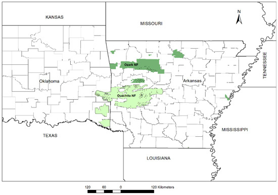
Figure 1.
Map showing the 196 out of 208 permanent plot locations of the natural even-aged Shortleaf pine (Pinus echinata Mill.) stand in Ozark (35) and Ouachita National Forest (161). The black dot in the map gives a general idea of plot locations but does not provide a precise location due to the clustering of circular plots at 36.3 m (120 ft.) apart with buffer strips in one site. The geographic location of 12 plots was missing.
The total sample consisted of 208 plots. Out of 208 plots, 40 plots were distributed in Ozark National Forest, and the rest of the plots were in Ouachita National Forest. Plots were remeasured every 4 to 6 years, and the last (sixth) measurement occurred during the period from 2012 to 2104. The survival status of each tree was recorded at each measurement. Variables, including diameter at breast height (dbh) (cm), tree height (HT) (meters), and the height to base of live crowns (meters) were recorded for each tree on each of the measurement plots. Each tree was classified as dominant, co-dominant, intermediate, or suppressed. The measurement sample plot was circular with a radius of 17.4 m (57.2 feet) and 0.0809 hectares (ha) (0.2 acres) in size. The measurement plots were surrounded by a buffer strip 10 m (33 feet) wide and received the same silvicultural treatments at establishment as the measurement plot. Before the fourth measurement, an ice storm event occurred, so ice-damaged plots (101) were excluded after the third measurement in this study. Most plots were re-thinned to their original basal area levels just after the third measurement, while a portion were left unthinned. The thinned basal area per hectare (m2ha−1) was deducted from the estimated basal area per hectare of the third measurement period. This deduction better reflects the competitive pressure experienced by the trees on the plot during the measurement interval subsequent to thinning. An average thinned basal area was 6.94 m2ha−1 with a range of 0.69–19.36 m2ha−1. The total number of trees available for mortality analysis at the beginning of each of the five measurements was 8288, 8078, 4027, 2470, and 2355 consecutively.
2.2. Model Development
2.2.1. Logistic Regression Model
In our data, the response variable ‘y’ represents mortality for an individual shortleaf pine tree and has values of 1 for trees that have died the measurement interval or 0 for trees that survived during that time with probabilities pi and 1 − pi, respectively. Since yi (an individual tree) is an independent Bernoulli random variable with parameter E{y} = p, the simple logistic regression form was used.
Taking log;
Hamilton and Edward [27] modified Equation (1) to Equation (2), which he used to fit the parameters for a logistic model to estimate the probability of mortality.
where p is the annual probability of mortality, x1, x2, …, xn are set of n predictor variables, β0, β1, …, βn are regression parameters to be estimated and exp(x) = ex where e is base of the natural logarithm. Many later researchers set p to the annual probability of survival (e.g., Monserud [21]). Equation (2) provides the probability of mortality rather than the probability of survival. The probability of survival would be 1 − p, because by definition, p is bounded by 0 and 1.
2.2.2. Variable Selection
For preliminary screening, the survival data were modeled using the SAS/PROC LOGISTIC procedure, a typical logistic regression model fit for data with dichotomous outcomes via the method of maximum likelihood [35,36]. A stepwise procedure in PROC LOGISTIC was used to select the best set of predictor variables at a significance level of α = 0.05 [35]. Initially, all possible predictor variables were tested (Table 1). Finally, stand age derived competition indices such as the ratio of stand basal area per hectare to stand or plot age (SBAG), the ratio of dbh to plot age (DAG), and quadratic mean diameter (QMD) were found to be highly significant with p < 0.0001, and more promising than other variables.

Table 1.
Summary of the variables for mortality of individual trees (n = total dead trees) of naturally occurring even-aged shortleaf pine stands in each measurement period from 1985 to 2014 in Ozark and Ouachita National Forests, USA.
For most plots, only a subsample of trees was selected to measure total height and crown length. Therefore, height prediction and crown ratio estimation models for shortleaf pine of Saud et al. [33] were used to predict the missing measurements for testing independent variables that use height and/or crown ratio. Summary statistics for the selected variables are given in Table 2. An interaction term was also included in the model. Though the interaction terms were highly significant (p < 0.0001) in the model, the performance of the model with interaction terms was not satisfactory in terms of chi-square (χ2) goodness of fit test value. Therefore, models with interaction terms are not discussed here.
Table 2.
Summary statistics of 25,218 individual trees used to fit mortality regression models from naturally occurring even-aged shortleaf pine stands from 1985 to 2014 in Ozark and Ouachita National Forests, USA.
To represent the possible effects of the thinning in the model, a THINHA = (Thinned basal area per hectare/(years since thinning) variable was created. Because the thinned basal area is divided by the number of years since thinning, this variable causes thinning effects to be reduced with time. In the thinning model, all of the above-mentioned variables were found to be significant along with THINHA, and these variables were used with and without interaction terms in alternative models.
2.2.3. Binary Logistic Regression Model and Iteratively Weighted Regression Model
Data from the remeasured plots include multi-year intervals in which tree survival or death is observed. Let ‘t’ be such an interval over which to observe tree death or survival. Monserud [21], Monserud and Sterba [22], and Hamilton and Edwards [27] described a model (Equation (2)) to estimate the probability of survival, assuming that survival time follows uniform distribution over the growth interval. The model of Equation (2) was modified to obtain Equation (3), ‘binary logistic regression model’, to predict mortality probability rather than survival probability where the response variable is mortality. This formulation is more consistent with biomedical practice (right censored data), and in a related work, we want to compare these methods to other methods available in the biomedical literature. Flewelling and Monserud [37] state that mortality is not a Markov process because a tree can only die once. However, survival is a Markov process. Therefore, “this property requires that all algebra be mediated in terms of survival, not mortality” [37]. Because of this, we modeled mortality (with tree death = 1) as 1 − p (tree survives to the end of the measurement period).
where pjt is the probability that tree j died during the measurement interval of t years, and the βi are parameters to be estimated.
Equation (3) was used to predict the mortality probability in different time intervals. When the interval t is zero or at the beginning of the growth period, the probability that the tree survives is 1, which means the tree is alive. Conversely, as t → +∞, the probability of survival decreases and eventually approaches zero [27,37]. The model with a thinning effect includes the variable THINHA in Equation (4). Both Equations (3) and (4) were used for the iteratively reweighted nonlinear regression model.
where the notations are as described above for Equation (3).
PROC NLIN is the major SAS procedure for nonlinear (or curvilinear) regression analysis [35]. The NLIN procedure fits nonlinear regression models and estimates the parameters by nonlinear least-squares or weighted nonlinear least squares [35]. Since mortality is a binary or Bernoulli random variable, it has variance pt (1 − pt), where pt is the probability of mortality during t years. The inverse of the variance, i.e., 1/(pt (1 − pt)) was used as a weight while fitting the nonlinear regression. McCullagh and Nedler [38] recommended iteratively reweighted regression as an effective procedure to find the maximum likelihood estimates for the mortality model. Equations (3) and (4) were used in what we term here as the “binary logistic model” and “binary thinned” by specifying a binary distribution with probability pt. The NLMIXED procedure in SAS [35] was used to fit the binary logistic regression model where no random effect was specified.
2.2.4. Mixed-Effects Model
A nonlinear mixed-effects modeling approach is to many forestry data sets by including plot-specific random effects for the repeated measurement or the longitudinal dataset. This statistical modeling approach consists of both fixed and random effects of parameters associated nonlinearly with the response variable in the model [33,39,40,41]. Furthermore, the mixed-effects modeling approach often helps to account for temporal and spatial correlation in the model, a special case in the longitudinal data collected from different sites. According to Lappi [40], mixed models work better when items in the datasets occur in groups. Grouped datasets may contain longitudinal or repeated measurements or can be defined as multilevel or block designs [41].
We also fitted the mixed-effects models to develop a model for the probability of mortality for shortleaf pine. The NLMIXED procedure in SAS [35] was used to fit the nonlinear mixed-effects models by specifying that the response variable had a binary distribution. We investigated random effects associated with the plot, additive to the intercept parameter, and the parameters associated with all variables of the model. The best results were obtained by adding random effect to the parameter associated with QMD without the thinning effect “binary mixed” model (Equation (5)), and associated with THINHA with the thinning effect “binary mixed thinned” model (Equation (6)).
where β0, β1, β2, β3, and β4, are parameters to be estimated for tree j on plot k, uk is the random effect associated with plot k distributed normally with mean 0 and variance σ2u and εjk is the error term with mean zero.
2.2.5. Model Evaluation and Accuracy
The Akaike information criteria (AIC) were used to select the best alternative models [42]. The AIC and log-likelihood were estimated as given below (Equations (7) and (8)), where d is the number of parameters in the model and l is the log-likelihood;
Once the fitted response function was obtained, a goodness-of-fit test was conducted to check the fitness of the response function. The fitted probability response was transferred to the probability of either 0 or 1, considering 0.5 as threshold probability. The estimated probability ≥0.5 was assigned as 1 to classify a tree mortality; otherwise, tree survival was signified. The chi-square (χ2) test is often used to evaluate the appropriateness of the model [43] that has a binary response variable. After obtaining parameter estimates, comparisons between observed and predicted numbers of live and dead trees were made using dbh classes with widths of five centimeters and labeled by the class midpoint. Based on these diameter classes, the models with the lowest AIC values were evaluated using the χ2 goodness-of-fit test (Equation (9)). The χ2 value by mid diameter classes was calculated as:
where Oj1 and Oj0 are the observed number of mortality and survival trees, respectively, in diameter class j. Similarly, Ej1 and Ej0 are the number of dead trees and surviving trees, respectively, in diameter class j expected from the model and c is the number of diameter classes.
Model prediction accuracy was evaluated using the principal of the Receiver Operating Characteristic (ROC) curve [44]. ROC analysis was conducted in R using ROCR package [42,44,45], and the area under the curve (AUC) was used to evaluate the model. We considered the threshold of 0.5 probability to obtain the area under the curve as mentioned above. The lower the AUC values, the better the model prediction accuracy. In the figure illustrating ROC, the vertical y-axis represents the true positive rate, which is called sensitivity. Sensitivity is the rate of probability for positive predictions given that a subject or an individual is positive. The horizontal x-axis represents the false positive rate, which is also specificity, and the rate of the probability to be predicted positive, given that a subject or an individual is negative. The false positive rate is also denoted as 1-specificity.
3. Results
3.1. Mortality
The mortality of shortleaf pine was 13.67% of the initial total sample population, from the plot establishment year 1985–1987 until the last sixth measurement period (2012–2014). The mortality rate was, on average, 3.73% for a measurement period or a growth length period (which could be from 4–6 years on individual plots). The mortality rate was 2.44%, 6.21%, 6.63%, 4.70%, and 1.95% for the five consecutive measurement periodss. The proportion of mortality trees was significantly different for at least one measurement period (df = 4, χ2 = 203.70, p < 0.001). Dead trees were highly distributed to the lower dbh ranges during each measurement period, i.e., from 10 to 20 cm (Table 1), with a high mortality rate in the first two measurement periods. The highest mortality rate occurred for the lower dbh class (median = 7.87 cm) during the second measurement period (Table 1), which could be due to the effects of competition as the density increased on the plots. In the second measurement period, 290 dead trees were found in mid-dbh class of 7.5 cm, and 79.3% of that mortality occurred in the young plot age classes ranging between 27–30 years with a high stand density, i.e., more than 2200 trees per hectare.
3.2. Iteratively Reweighted Nonlinear Regression Model and Binary Logistic Regression Model
The parameter estimates for the binary logistic model (Equation (3)) were all significant with p-value < 0.0001, and the model had an AIC value of 7983 (Table 3). The iteratively reweighted regression model had similar parameter estimates as Equation (3). This similarity was as expected since these are simply two different ways of solving the same likelihood function. However, standard errors and the confidence intervals were slightly different. It was found that the standard errors for the parameter estimates of the binary logistic model (Equation (3)) were smaller by an average of 33%, making the confidence interval narrower than that of the reweighted regression model.
Table 3.
Parameter estimates (standard errors) of the binary logistic regression model (Equation (3)) and binary thinned model (Equation (4)) for mortality prediction of an individual tree of naturally occurring even-aged shortleaf pine stand in Ozark and Ouachita National Forest, USA.
The parameter estimates of the binary thinned model (Equation (4)) were all significant with a p-value < 0.0001, and an AIC value of 7878 (Table 3). As mentioned above, the reweighted regression models with thinning effect also had parameter estimates similar to those of the binary model (Equation (4)). The standard errors of the parameter estimates in the binary model with a thinning effect were also found to be almost 37% smaller than the iteratively reweighted regression model form with the thinning effect. Therefore, the binary model was preferred over the iteratively reweighted regression estimates.
3.3. Parameter Estimation Using a Nonlinear Mixed Model
In the mixed-effects modeling approach, the random effect of the plot associated with variable QMD was found to be better than other alternative models (not reported) with all parameter estimates highly significant (p-value < 0.0001). It was found that the AIC value of binary mixed model (Equation (5)) was 7498. The parameter estimates and AIC value of Equation (5) is shown in Table 4. The variance component (σ2uk = 0.0024) associated with the parameter b3 of QMD was significant, with a confidence interval of [0.0017, 0.0033]. It was found that the parameter b1 of SBAG was highly positively correlated (0.82) with b3 of QMD. The correlation and covariance matrices of the binary mixed model (Equation (5)) are shown in Table 5.
Table 4.
Parameter estimates (standard errors), and AIC value for mixed-effects approach model; binary mixed (Equation (5)) and binary mixed thinned (Equation (6)) for prediction of mortality probability in natural stands of shortleaf pine in Ozark and Ouachita National Forest, USA.
Table 5.
Matrix of correlations and covariance for mixed-effects approach model; binary mixed (Equation (5)) and binary mixed thinned (Equation (6)).The values above diagonal are correlation and those below are covariance.
In the mixed-effects model with thinning effect (Equation (6)), all parameter estimates were highly significant except the random effect of the plot associated with the parameter (b2) of DAG. The AIC value of the binary mixed thinned models was similar for the random effect associated with variable THINHA and SBAG. Likewise, the AIC value with random effect associated with QMD and intercept was similar but smaller than former variables. For the purpose of discussion, the parameter estimates and AIC value of Equation (6), and random effect associated with SBAG and QMD are shown in Table 4. However, the random effect associated with THINHA (Equation (6)) provided a better chi-square test value for the prediction than models with lower AIC values. Therefore, Equation (6) was selected as a binary mixed thinned model. The variance component (σ2u = 0.1518) associated with parameter b4 of THINHA was significant, with a confidence interval of [0.0977, 0.2060]. It was also found that the parameter b1 of SBAG was positively correlated (0.85) with b3 of QMD. The correlation and covariance matrices of the binary mixed thinned model (Equation (6)) are shown in Table 5.
3.4. Mortality Prediction
The chi-square test statistic has two components, one based on observed minus expected mortality, and the other based on observed minus expected survival. However, individual survival and mortality components were sometimes of a more modest magnitude. The estimated χ2 goodness of fit test value for both significant models (Equations (3) and (4)) was less than tabulated (χ2 (9, 0.05) =16.91) for survival prediction in mid-dbh class, but it was not for mortality prediction. The total χ2 test value was 24.62 for binary logistic model (Equation (3)) with χ2 = 1.57 for survival prediction and χ2 = 23.05 for mortality prediction in mid-dbh class. Similarly, the total χ2 test value was 33.02 for binary thinned model (Equation (4)) with χ2 = 2.01 for survival prediction and χ2 = 30.01 for mortality prediction in mid-dbh class.
The χ2 test value was larger for binary mixed and binary mixed thinned models than the binary model. In the binary mixed model, the random effect associated with QMD (Equation (5)) had a total χ2 test value of 52.35, with χ2 = 3.31 for survival prediction and χ2 = 49.04 for mortality prediction for mid-dbh. In binary mixed thinned, the random effect associated with THINHA (Equation (6)) had a total χ2 test value of 61.60, with χ2 = 2.54 for survival prediction and χ2 = 59.06 for mortality prediction for mid-dbh class. However, the total χ2 test value was substantially larger for the alternative binary mixed models with the thinning effect. For example, the total χ2 test value was 88.34 and 255.54 for the random effect associated with SBAG and QMD, respectively.
Both the binary logistic model and binary thinned model showed better fit in terms of mortality curve with the observed mortality than for the mixed-effects models (Figure 2a). The percentage difference in observed and predicted mortality for each mid-dbh class showed that the binary logistic model provided a marginally better fit in predicting mortality than the binary thinned model (Figure 2b and Table 6). In the mixed-effects model approach, the binary mixed model appeared to have greater percentage differences in mortality prediction than binary mixed thinned (Figure 2b). All models (Equations (3)–(6)) under predicted mortality for mid-dbh classes at 2.5 cm and 7.5 cm, respectively (Figure 2b and Table 6). The total number of predicted mortality trees was nine trees greater than observed dead trees for the binary logistic model, and it was eight trees greater than observed for the binary thinned model (Table 6). However, the total number of predicted mortality trees was 161 trees less than the observed dead trees for the binary mixed model, but 15 trees greater for the binary mixed thinned model (Table 6).
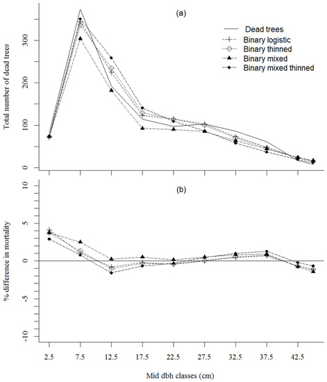
Figure 2.
Predicted total number dead trees (a), and the percentage difference of observed and predicted number dead trees (b) for each mid diameter class by binary logistic model fit and mixed-effects model fit for with and without thinning effect for shortleaf pine in Ozark and Ouachita National Forest, USA.
Table 6.
Observed and predicted survival and mortality by five centimeter classes from a nonlinear approach of binary logistic model fit, and a mixed-effects model fit for with and without thinning effect for shortleaf pine in Ozark and Ouachita National Forest, USA.
3.5. Model Accuracy
Examination of the ROC curve showed that the area under the curve (AUC) for the models with thinning effect (Equations (4) and (6)) were better than in the models without the thinning effect (Figure 3). Figure 3 indicates that the mixed-effects model without thinning effects was slightly better than the binary model without thinning effects. However, the binary model with thinning effects was slightly better according to the AUC criterion than the mixed-effects model with thinning effects, and was the best model by a small margin according to the AUC criterion. The AUC of all models indicated that the model has a reasonably good ability to discriminate the mortality risk of an even-aged individual shortleaf pine tree growing in a natural forest stand.
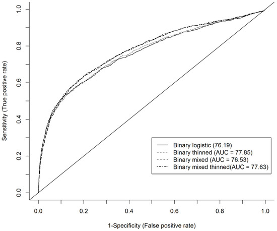
Figure 3.
ROC curve showing area under curve (AUC) for binary models and mixed-effects models for mortality prediction of even aged natural stand of shortleaf pine in Ozark and Ouachita National Forests, USA.
3.6. Influence of Variables in Predicting Mortality
The relative influence of variables in predicting mortality was similar in all models tested with a thinning effect and those without a thinning effect. Figure 4 illustrates the behavior of mortality predictions for classes of several of the important variables used in modeling. The predicted probabilities were from binary logistic (Equation (3)) except THINHA from binary thinned (Equation (4)). Increasing value for stand-level variables was associated with increased mortality probability (Figure 4a,c,d), while increasing values of individual tree level variables were associated with decreasing mortality probability (Figure 4b). The change in mortality risk was very small for modestly increasing values of SBAG, QMD, and THINHA. The predicted mortality over the measurement-length period showed that the mortality risk was nearly 5% for the median of the population of trees belonging to the uppermost mid-class for SBAG (Figure 4a), QMD (Figure 4c), and THINHA (Figure 4d). The influence of thinning variable in mortality could be possible due to the logging effect. Similarly, the mortality risk was 5% for the median population of trees belonging to the lower mid-class of DAG (Figure 4b). The influences on predicting mortality by each variable could be more significant for some individual trees than shown in Figure 4 because some of the predicted mortalities were beyond the upper whisker of the boxplot for all variables.
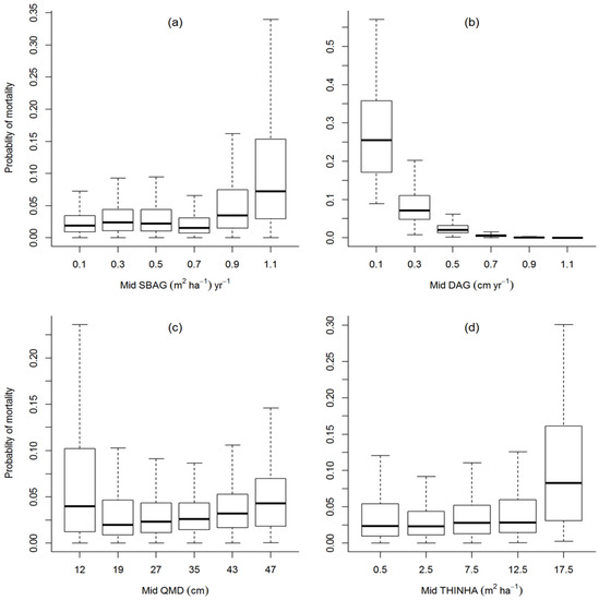
Figure 4.
Box plot showing the predicted probability of mortality against the variables; (a) SBAG, (b) DAG, (c) QMD, and (d) THINHA, used in the model at their mid-class ranges. The boxplot for variable ‘THINHA ‘was plotted from the parameter estimates of binary thinned (Equation (4)), while other boxplots were plotted from the parameter estimates of the binary logistic model (Equation (3)).
Figure 5 shows predicted annual survival with respect to change in selected individual variables while all other variables are held constant at their mean values for the dataset. The reference of all variables for Figure 5 is as discussed above for Figure 3. The variable that appeared to have the most significant impact on annual survival probability over the range plotted was only DAG. Although SBAG, QMD, and THINHA showed a very small change in survival probability for increasing values, SBAG showed a relatively smaller decreasing annual survival probability compared to the other two (Figure 5a,c,d). The increased value of the variable SBAG (>1.4 m2 ha−1/years) and QMD (>50 cm) are likely to increase the stand-level competition and influence the survival of a suppressed tree by 5%. The ratio of diameter to stand plot age greater than 0.3 (cm year−1) showed stable and better survival probability for an individual tree (Figure 5b).
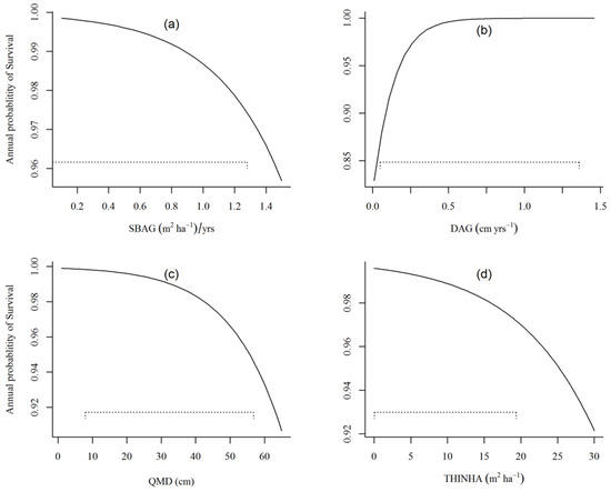
Figure 5.
Influence of a variable in predicting annual survival probability while fixing all other independent variables; (a) SBAG, (b) DAG, (c) QMD, and (d) THINHA, as constant equal to their data means. The plot for THINHA was plotted using parameter estimates of binary thinned (Equation (4)), while other plots were plotted using parameter estimates of binary logistic (Equation (3)).
4. Discussion
The mortality curve (Figure 2a,b) is not U-shaped or reversed J-shaped, which is often presumed to be the main alternative relationship for mortality trends [46,47,48]. This happened because the highest mortality occurred at lower mid-dbh classes (Table 6). The mortality was almost 9.2% for multi-year measurement intervals from the 7.5 and 12.5 cm mid-dbh classes though subsequently increasing dbh classes displayed a decreased mortality rate. A similar pattern of higher mortality rate (7%) at lower dbh class (5–15 cm) was observed ten years after planting shortleaf pine in Oklahoma [49]. This likely confirms that it is possible to obtain a high spike in mortality in lower dbh classes (Figure 2a,b). If the mortality from the lower mid-dbh class is ignored or merged into classes with wider intervals (10 cm), then Figure 2 could display a reversed J-shaped curve. Another factor that may influence the mortality trends in this study is the fact that there were many “young-aged” plots containing large numbers of small trees per hectare at the beginning of the study. As these plots approached competition-induced mortality densities, significant numbers of mortality trees in mid-range dbh classes probably occurred. This increased mortality could result from a change in stand-age derived competition indices due to the available spacing between trees within a plot. It also indicated that competition-induced mortality affects the survival of trees within specific diameter ranges as stand density approaches the upper limit [4]. However, stand dynamics change over time and strongly influence competition indices due to spacing, which determines a tree’s growth and survival [46,49,50,51].
Our results demonstrate that thinning from below significantly affected the mortality prediction, but it may not greatly influence predictions about the probability of individual tree mortality. Part of the reason may be that thinning from below mimics inter-tree competition, leaving large-sized trees to occupy extensive canopy cover. In 1995–1997, as a process of thinning treatment, trees from intermediate and overtopped canopy classes were removed. Over the decadal period of changing stand structure, the stand experienced the diminishing effect of thinning in tree mortality. Similar to our study, the mortality in the thinning from below was not significantly higher than thinning from above in the red pine (Pinus resinosa) forest in Minnesota, USA [4]. However, thinning from above with varying intensity increases mortality in the first decadal period [1], though the growth response of the residual trees shows a better growth response [19]. The gap created by thinning could initiate windthrow mortality that varies with thinning intensity and topographic features. Such tree mortality is better explained by the individual tree attributes such as tree height, breast height, slenderness, developmental stage, and tree species [17]. However, mortality risk was associated with the thinning applied. This increased risk might be due to the logging damage effects on the residual trees coupled with windthrow and other unknown environmental stress [4,17]. Additionally, because thinning affects tree attributes such as individual tree basal area, the effects of thinning on individual tree survival may be largely represented by changes in these tree attributes with age so that an additional thinning variable does not add much more predictive power.
Mortality or survival prediction models could potentially include a variety of different ratios and stand competition indices as predictor variables [8,12,13,16,22,25]. We also tested a variety of variables, not all of which were discussed above, but discarded several for various reasons. There were sets of models provided by stepwise logistic regression which had better AUC and AIC values in the binary logistic model form than the finally selected models, but they performed poorly in the chi-square goodness of fit test. Examples of these included binary logistic model with variables (a) CRT, RAQD, BAHA (basal area per hectare) and DAG, and (b) HDR, BAHA, QMD (quadratic mean diameter) and DAG. Although the diameter at breast height is an important factor [4,6,12], the derived factors with age better explained the probability of tree mortality with stand developmental age. As diameter increases with age, larger trees can withstand the canopy competition and have better survival chances than small stems [4,6,7].
In the alternative binary mixed thinned models, the random effect associated with intercept and QMD had smaller and similar AIC, but their performance in the χ2 test was poorer than with a random effect associated with THINHA (Equation (6)). It appeared from the χ2 test results that the mixed-effects modeling approach was not satisfactory for a natural stand with longer remeasurement intervals. This approach may be better for survival prediction with shorter remeasurement periods with plantation tree species as in Rose et al. [51]. In a similar study by Groom et al. [52] for predicting Douglas-fir mortality the authors also reported that the mixed-effects model performed poorly in a goodness of fit test.
There can be an apparent conflict between using the AIC criterion and the χ2 goodness of fit test to evaluate model performance. The mixed model appeared to be better than the binary model using the AIC criterion but did not perform as well in the χ2 goodness of fit test is used to evaluate model performance. Part of the reason may be that the probabilities are being evaluated for the mixed model using the fixed-parameter estimates only to conduct the chi-square test. However, the AIC evaluation, of course, includes the random-effects parameters. In typical model applications, the random effect for a particular forest would not be known. In other mixed model applications to forest resources, for example, the dbh-height relationship, one often may be able to calibrate a mixed model by estimating random parameters with locally obtained data [53,54]. However, applying a mortality model would usually be challenging because remeasured plots are required to calibrate the random effect but are typically unavailable. Furthermore, some forest-modeling literature indicates that OLS models without mixed-effects may be preferred to mixed-effects models if calibration using locally available data cannot be applied [51,52,53,54,55,56]. However, these studies did not address mortality models specifically.
The high χ2 test values for binary models suggest that the model predicts significantly different number of dead trees than were observed for one or more mid-dbh classes (Table 6). The estimated χ2 test value for this binary logistic model (Equation(3)) and binary thinned model (Equation (4)) could be marginally reduced by increasing the dbh class width from five cm to ten cm. For example, the reduced total χ2 test value for Equation (3) was 21.5, and for Equation (4), it was 29.89. The χ2 test value cannot always be made small enough to fail to reject the mortality model for all tree species even with large dbh intervals (10 cm) [22,56]. The large χ2 test value obtained here was possibly due to the variability in measured variables of natural shortleaf pine stands in the dataset used to develop these mortality prediction models. The better prediction obtained from these models will help simulate the stand growth change to evaluate the effect of climate change better, and potential carbon sequestration due to stand-age derived competition indices of a natural stand of shortleaf pine.
5. Conclusions
Our findings suggest that an independent variable that provides variation in the point estimates of their associated parameters, either relatively small or very large in the combination of the other variables in a model, might be helpful to predict the better mortality probability of an individual tree. Stand-age derived competition indices that change with age, such as SBAG and DAG, and without age QMD were more influential in predicting mortality than other variables considered in this study. Ideally, the same independent variables would be important whether the dependent variable in the probability prediction model was survival or mortality. The binary model appears to be better for predicting the probability of mortality than the mixed-effects model. A model showing thinning effects was not very strong because the thinning was conducted from below, and thinning intensity varied among the plots. However, mortality risk was associated with the thinning applied. Rather than using the thinning effect variable, accounting for the thinned basal area occurred in the value of residual stand basal area, the binary model resulted in better performance with a chi-square test based on mortality within dbh classes than other models considered in this study. This binary logistic model can be used to predict the annual mortality or survival rate of individual trees of even-aged shortleaf pine forests. This binary logistic regression model performed better than alternative models in this study and could be tested for use in a shortleaf pine growth simulation such as the Shortleaf Pine Stand Simulator (SLPSS) [9], a distance-independent individual tree growth simulator for naturally occurring shortleaf pine. In the future, considering the climate effects together with the thinning effects might be beneficial in predicting individual tree mortality for individual shortleaf pine trees in naturally occurring forests.
Author Contributions
T.B.L. and J.M.G. conceived and designed the experiments; T.B.L. and J.M.G. collected field data; P.S. and S.S. curated the data and outlined methodology; P.S. analyzed and wrote the paper; T.B.L. and J.M.G. reviewed and edited the paper. All authors have read and agreed to the published version of the manuscript.
Funding
This research was supported by the Department of Natural Resource Ecology and Management) at Oklahoma State University (OSU) (Project # OKLO-2843) and USDA Forest Service Southern Research Station (UAFS) at Monticello, Arkansas (Project # 16-CA-11330123-003). This article has been approved for publication by the Oklahoma Agricultural Experiment Station.
Institutional Review Board Statement
Not applicable.
Informed Consent Statement
Not applicable.
Data Availability Statement
Not applicable.
Acknowledgments
We would like to thank Bob Heinemann, Randy Holeman, Dennis Wilson and Keith Anderson of the Oklahoma State University Kiamichi Research Station and all other staff and crew members for collecting data from 1984 to 2014. We also would like to thank the Division of Agricultural and Extension, University of Arkansas System, and Arkansas Forest Resource Center for their funding support to publish this research work. We also like to thank unknown reviewers for their valuable comments and suggestions.
Conflicts of Interest
The authors declare no conflict of interest.
References
- Roberts, L.J.; Burnett, R.; Tietz, J.; Veloz, S. Recent drought and tree mortality effects on the avian community in southern Sierra Nevada: A glimpse of the future? Ecol. Appl. 2019, 29, e01848. [Google Scholar] [CrossRef]
- Saud, P.; Wang, J.; Lin, W.; Sharma, B.D.; Hartley, D.S. A life cycle analysis of forest carbon balance and carbon emissions of timber harvesting in West Virgina. Wood Fiber Sci. 2013, 45, 250–267. [Google Scholar]
- Ameray, A.; Bergeron, Y.; Valeria, O.; Girona, M.M.; Cavard, X. Forest carbon management: A review of silvicultural practices and management strategies across boreal, temperate and tropical forests. Curr. For. Rep. 2021, 7, 245–266. [Google Scholar] [CrossRef]
- Powers, M.D.; Palik, B.J.; Bardford, J.B.; Fraver, S.; Webster, C.R. Thinning method and intensity influence long-term motrality trends in a red pine forest. For. Ecol. Manag. 2010, 260, 1138–1148. [Google Scholar] [CrossRef]
- Saud, P.; Lynch, T.B.; Guldin, J.M. Twenty five years long survival analysis of an individual shortleaf pine trees. In Proceedings of the 18th Biennial Southern Silvicultural Research Conference, Knoxville, TN, USA, 2–5 March 2015; Schweitzer, C.J., Clatterbuck, W.K., Oswalt, C.M., Eds.; U.S. Department of Agriculture, Forest Service, Southern Research Station: Asheville, NC, USA; pp. 555–557. [Google Scholar]
- Ruel, J.C.; Gardiner, B. Mortaltiy patterns after different levels of harvesting of old-growth boreal. For. Ecol. Manag. 2019, 448, 346–354. [Google Scholar] [CrossRef]
- Oliver, C.D. Forest development in North America following major disturbances. For. Ecol. Manag. 1981, 3, 153–168. [Google Scholar] [CrossRef]
- Lynch, T.B.; Hitch, K.L.; Huebschmann, M.M.; Murphy, P.A. An Individual-Tree Growth and Yield Prediction System for Even-Aged Natural Shortleaf Pine Forests. South. J. Appl. For. 1999, 23, 203–211. [Google Scholar] [CrossRef]
- Yang, Y.; Titus, S.J.; Huang, S. Modeling individual tree mortality for white spruce in Alberta. Ecol. Model. 2003, 163, 209–222. [Google Scholar] [CrossRef]
- Fortin, M.; Bédard, S.; Deblois, J.; Meunier, S. Predicting individual tree mortality in northern hardwood stands under unevenaged management in southern Quebec, Canada. Ann. For. Sci. 2008, 65, 205. [Google Scholar] [CrossRef]
- Peet, R.K.; Christensen, N.L. Competition and Tree Death. Bioscience 1987, 37, 586–595. [Google Scholar] [CrossRef]
- Zhao, D.; Borders, B.; Wilson, M.; Rathbun, S.L. Modeling neighborhood effects on the growth and survival of individual trees in a natural temperate species-rich forest. Ecol. Model. 2006, 196, 90–102. [Google Scholar] [CrossRef]
- Cao, Q.V.; Strub, M. Evaluation of four methods to estimate parameters of an annual tree survival and diameter growth model. For. Sci. 2008, 54, 617–624. [Google Scholar]
- Girona, M.M.; Morin, H.; Lussier, J.-M.; Ruel, J.-C. Post-cutting Mortality Following Experimental Silvicultural Treatments in Unmanaged Boreal Forest Stands. Front. For. Glob. Chang. 2019, 2, 4. [Google Scholar] [CrossRef]
- Bravo-Oviedo, A.; Sterba, H.; del Rio, M.; Bravo, F. Competition-induced mortality for Mediterranean Pinus pinaster Ait. and P. sylvestris L. For. Ecol. Manag. 2006, 222, 88–98. [Google Scholar] [CrossRef]
- Zhao, D.; Borders, B.; Wilson, M. Individual-tree diameter growth and mortality models for bottomland mixed-species hardwood stands in the lower Mississippi alluvial valley. For. Ecol. Manag. 2004, 199, 307–322. [Google Scholar] [CrossRef]
- Lavoie, S.; Ruel, J.-C.; Bergeron, Y.; Harvey, B.D. Windthrow after group and dispersed tree retention in eastern Canada. For. Ecol. Manag. 2012, 269, 158–167. [Google Scholar] [CrossRef]
- Moussaoui, L.; LeDuc, A.; Girona, M.M.; Bélisle, A.C.; LaFleur, B.; Fenton, N.J.; Bergeron, Y. Success Factors for Experimental Partial Harvesting in Unmanaged Boreal Forest: 10-Year Stand Yield Results. Forests 2020, 11, 1199. [Google Scholar] [CrossRef]
- Girona, M.M.; Morina, H.; Lussier, J.M.; Walsh, D. Radial growth response of black spruce stands ten years after experimental shelterwoods and seed-tree cuttings in Boreal Forest. Forests 2016, 7, 240. [Google Scholar] [CrossRef]
- Bailey, R.L.; Borders, B.E.; Ware, K.D.; Jones, E.P. A compatible model relating slash pine plantation survival to density, age, site index, and type and intensity of thinning. For. Sci. 1985, 31, 180–189. [Google Scholar]
- Monserud, R.A. Simulation of forest tree mortality. For. Sci. 1976, 22, 438–444. [Google Scholar]
- Monserud, R.A.; Sterba, H. Modeling individual tree mortality for Austrian forest species. For. Ecol. Manag. 1999, 113, 109–123. [Google Scholar] [CrossRef]
- Cao, Q.V. Prediction of annual diameter growth and survival for individual trees from periodic measurements. For. Sci. 2000, 46, 127–131. [Google Scholar]
- Gumpretz, L.; Pye, M. Logistic regression for southern pin beetle outbreaks with spatial and temporal autocorrelation. For. Sci. 2000, 46, 95–107. [Google Scholar]
- Crecente-Campo, F.; Soares, P.; Tomé, M.; Diéguez-Aranda, U. Modelling annual individual-tree growth and mortality of Scots pine with data obtained at irregular measurement intervals and containing missing observations. For. Ecol. Manag. 2010, 260, 1965–1974. [Google Scholar] [CrossRef]
- Efron, B. Logistic regression, survival analysis, and the Kaplan-Meier curve. J. Am. Stat. Assoc. 1988, 83, 414–425. [Google Scholar] [CrossRef]
- Zhang, D.; Huebschmann, M.M.; Lynch, T.B.; Guldin, J.M. Growth projection and valuation of restoration of the shortleaf pine–Bluestem grass ecosystem. For. Policy Econ. 2012, 20, 10–15. [Google Scholar] [CrossRef]
- Yao, X.; Titus, S.J.; Macdonald, S.E. A generalized logistic model of individual tree mortality for aspen, white spruce, and lodgepole pine in Alberta mixedwood forests. Can. J. For. Res. 2001, 31, 283–291. [Google Scholar] [CrossRef]
- Huebschmann, M.M.; Lynch, T.B.; Murphy, P.A. Shortleaf Pine Stand Simulator: An Even-Aged Natural Shortleaf Pine Growth and Yield Model User’s Manual; Oklahoma State University: Stillwater, OK, USA, 1998; 25p. [Google Scholar]
- Lynch, T.B.; Huebschmann, M.M.; Murphy, P.A. A survival model for individual shortleaf pine trees in even-aged natural stands. In Proceedings of the International Conference on Integrated Resource Inventories in the 21st Century, Grove Boise, ID, USA, 16–20 August 1988; Hanse, M., Burk, T., Eds.; Gen. Tech. Rep. NC-212. Dept. of Agriculture, Forest Service, North Central Forest Experiment Station: St. Paul, MN, USA; pp. 533–538. [Google Scholar]
- Lynch, T.B.; Murphy, P.A. A Compatible Height Prediction and Projection System for Individual Trees in Natural, Even-Aged Shortleaf Pine Stands. For. Sci. 1995, 41, 194–209. [Google Scholar] [CrossRef]
- Saud, P.; Lynch, T.B.; Anup, K.C.; Guldin, J.M. Using quadratic mean diameter and relative spacing index to enhance height–Diameter and crown ratio models fitted to longitudinal data. For. Int. J. For. Res. 2016, 89, 215–229. [Google Scholar] [CrossRef]
- Murphy, P.A. Growth and yield of shortleaf pine. In Proceedings of the Symposium on the Shortleaf Pine Ecosystem, Little Rock, AR, USA, 31 March–12 April 1986; Murphy, P.A., Ed.; Southern Forest Experiment Station, Arkansas Cooperative Extension Service, UAM: Monticello, AR, USA, 1986; pp. 159–177. [Google Scholar]
- SAS Institute, Inc. SAS Online Help Documentation; SAS Institute, Inc.: Cary, NC, USA; Available online: http://support.sas.com/documentation/onlinedoc/guide/ (accessed on 3 September 2014).
- Allison, P.D. Logistic Regression Using the SAS System: Theory and Applications, 2nd ed.; SAS® Publishing: Cary, NC, USA, 2001; 288p. [Google Scholar]
- Hamilton, D.A.; Edwards, B.M. Modeling the Probability of Individual Tree Mortality; Intermountain Forest and Range Experiment Station, Forest Service, U.S. Deptartment of Agriculture: Ogden, UT, USA, 1976; p. 22. [CrossRef]
- Flewelling, J.W.; Monserud, R.A. Comparing methods for modeling tree mortality. In Proceedings of the Second Forest Vegetation Simulator Conference; USDA For Serv Proceedings RMRS-P-25; USDA Forest Service, Rocky Mountain Research Station: Ogden, UT, USA; pp. 168–175.
- McCullagh, P.; Nelder, J.A. Generalized Linear Models, 2nd ed.; Chapman and Hall: New York, NY, USA, 1989; 511p. [Google Scholar]
- Wolfinger, R.D. Fitting nonlinear mixed models with the new NLMIXED procedure. In Proceedings of the 24th Annual SAS Users Group International Conference (SUGI 24), Miami Beach, FL, USA, 11–14 April 1999; pp. 278–284. [Google Scholar]
- Lappi, J. A multivariate, non-parametric stem-curve prediction method. Can. J. For. Res. 2006, 36, 291–301. [Google Scholar] [CrossRef]
- Pinheiro, J.C.; Bates, D.M. Mixed-Effects Models in S and S-Plus. Springer: New York, NY, USA, 2008; 528p. [Google Scholar]
- Sing, T.; Sander, O.; Beerenwinkel, N.; Lengauer, T. ROCR: Visualizing classifier performance in R. Bioinformatics 2005, 21, 3940–3941. [Google Scholar] [CrossRef] [PubMed]
- Neter, J.; Maynes, E.S. On the appropriateness of the correlation coefficient with a 0, 1 dependent variable. J. Am. Stat. Assoc. 1970, 65, 501–509. [Google Scholar] [CrossRef]
- Metz, C.E. Basic principles of ROC analysis. Semin. Nucl. Med. 1978, 8, 283–298. [Google Scholar] [CrossRef]
- R Development Core Team. R: A Language and Environment for Statistical Computing; R Foundation for Statistical Computing: Vienna, Austria, 2013; ISBN 3-900051-07. Available online: http://www.R-project.org (accessed on 25 January 2019).
- Coomes, D.A.; Duncan, R.P.; Allen, R.B.; Truscott, J. Disturbances prevent stem size-density distributions in natural forests from following scaling relationships. Ecol. Lett. 2003, 6, 980–989. [Google Scholar] [CrossRef]
- Woodall, C.; Grambsch, P.; Thomas, W. Applying survival analysis to a large-scale forest inventory for assessment of tree mortality in Minnesota. Ecol. Model. 2005, 189, 199–208. [Google Scholar] [CrossRef]
- Westphal, C.; Tremer, N.; Oheimb, G.V.; Hansen, J.; Gadow, K.V.; Härdtle, W. Is the reverse J-shaped diameter distribution uni-versally applicable in European virgin beech forests? For. Ecol. Manag. 2006, 223, 75–83. [Google Scholar] [CrossRef]
- Dipesh, K.; Will, R.E.; Lynch, T.B.; Heinemann, R.; Holeman, R. Comparison of Loblolly, Shortleaf, and Pitch X Loblolly Pine Plantations Growing in Oklahoma. For. Sci. 2015, 61, 540–547. [Google Scholar] [CrossRef]
- Buford, M.A. Performance of four yield models for predicting stand dynamics of a 30-year-old loblolly pine (Pinus taeda L.) spacing study. For. Ecol. Manag. 1991, 46, 23–38. [Google Scholar] [CrossRef]
- Rose, C.E.; Hall, D.B.; Shiver, B.D.; Clutter, M.L.; Borders, B. A multilevel approach to individual tree survival prediction. For. Sci. 2006, 52, 31–43. [Google Scholar]
- Groom, J.D.; Hann, D.W.; Temesgen, H. Evaluation of mixed-effects models for predicting Douglas-fir mortality. For. Ecol. Manag. 2012, 276, 139–145. [Google Scholar] [CrossRef]
- Lynch, T.B.; Holley, A.G.; Stevenson, D.J. A Random-Parameter Height-Dbh Model for Cherrybark Oak. South. J. Appl. For. 2005, 29, 22–26. [Google Scholar] [CrossRef]
- Lynch, T.B.; Budhathoki, C.; Wittwer, R.F. Relationships between Height, Diameter, and Crown for Eastern Cottonwood (Populus Deltoides) in a Great Plains Riparian Ecosystem. West. J. Appl. For. 2012, 27, 176–186. [Google Scholar] [CrossRef]
- Monleon, V.J. A hierarchical linear model for tree height prediction. In Proceedings of the 2003 Joint Statistical Meetings-Section Section on Statistics and the Environment, San Francisco, CA, USA, 3–7 August 2003; pp. 2865–2869. [Google Scholar]
- Temesgen, H.; Mitchell, S.J. An Individual-Tree Mortality Model for Complex Stands of Southeastern British Columbia. West. J. Appl. For. 2005, 20, 101–109. [Google Scholar] [CrossRef]


Publisher’s Note: MDPI stays neutral with regard to jurisdictional claims in published maps and institutional affiliations. |
© 2022 by the authors. Licensee MDPI, Basel, Switzerland. This article is an open access article distributed under the terms and conditions of the Creative Commons Attribution (CC BY) license (https://creativecommons.org/licenses/by/4.0/).