Article

Reproducibility of Stress Wave and Electrical Resistivity Tomography for Tree Assessment

Faculty of Resource Management, University of Applied Sciences and Arts, 37077 Göttingen, Germany
Forests 2022, 13(2), 295; https://doi.org/10.3390/f13020295
Submission received: 31 December 2021 / Revised: 6 February 2022 / Accepted: 8 February 2022 / Published: 12 February 2022
(This article belongs to the Special Issue Tree Stability and Tree Risk Analysis)

Abstract

:
(1) Background: Tomography is widely used in tree risk assessment and forest ecology. Tomograms should be accurate, repeatable and comparable between consecutive measurements. This is the first longitudinal study addressing reproducibility over a period of several years and the key factors influencing it, from raw data to final tomograms. (2) Methods: Trees were either repeatedly measured by the same researcher over periods of hours to months, by different researchers using either the same or a new installation of the same equipment, or with different tomographs. (3) Results: Overall, differences between tomograms were small and without impact on the assessment of the safety of the tree. Between initial and follow-up measurements after 2 to 5 years, the coefficients of correlation of stress wave velocity ranged from 0.75 to 0.96, those of loss in section modulus estimated from tomograms ranged from 0.82 to 0.93. The coefficient of correlation of repeated sapwood area estimates with electrical resistivity tomography was 0.97. The major cause of deviations was variation in the sensor positions between repeated tomographies, and, for electrical resistivity tomography, variation of temperature. (4) Conclusion: Provided that sensor positions are accurately recorded and documented, tomograms can reliably be repeated by different assessors over periods of years. Assessments based on complex calculations like loss of section modulus should be treated with caution, because they accumulate and amplify all sources of variation.

1. Introduction

Property owners and government agencies have a legal duty of care for their trees and thus have to manage risks related to these trees. A central part of tree risk management is tree risk assessment. The risk of the vast majority of trees can be assessed visually during a basic assessment, but when the likelihood of failure remains uncertain after a visual inspection, a number of tools can be used for an advanced assessment to measure the extent of decay, loss of strength, or anchorage. Tomographs are such tools that have been widely used in tree risk assessment and research in urban forestry in recent years (e.g., [1,2,3,4,5]). They are used to map internal decay non-destructively. Sonic tomographs (SoT) measure the time-of-flight of signals (t) to produce a map of apparent absolute or relative stress wave velocity (v), which will reveal areas of sound wood, if they can be traversed by stress waves on a straight path from one sensor to another. Electrical resistivity tomography (ERT) is a method to determine the spatial distribution of electric resistivity ( ρ ) non-destructively. In trees, results mainly correlate with ion and moisture content of the wood (e.g., [2,3,4]) and, to a lesser degree, wood temperature. In urban tree risk assessment ERT is used to aid the interpretation of results from SoT [6].
In tree risk assessment, tomograms are usually assessed with thresholds of residual wall thickness [7,8] or used in quantitative mechanical evaluations of the tomogram in terms of the section modulus (Z) or its resistance to bending [9]. Because the contribution of any part of the cross-section to the second moment of area increases with the square of its distance to the neutral axis of the stem (s. Equation (2)), even apparently small variations in the input to these calculations may result in large variation in their result [10,11].
A source of such variations within tomograms common to both methods is the distance between measurement points. Stress wave velocity is calculated from the time-of-flight (measured by the sensors), and the distance between those sensors (measured by the operator), while in electrical resistivity tomography, apparent resistivity is estimated from resistance between electrode pairs and electrode positions. A further source of variation between tomograms are the changes in sensor position that are unavoidable when measurements are repeated after several years, possibly by different operators.
Seasonal and diurnal changes in wood moisture and temperature could add further variation to tomograms. However, effects of wood moisture on v and resulting SoT of living trees are generally low [12,13,14,15] and the impact of declining temperature on stress wave velocity and tomograms is negligible as long as wood is not frozen [16].
Stem electrical resistivity, on the other hand, changes significantly with temperature [17,18] and seasonally changing resistivity has been described for Fagus sylvatica by [19], who found different pattern of change in sap wood and heart wood. Similarly, wood moisture content has a significant effect on ρ and resulting tomograms [17,18].
When technical devices support decision making in tree risk management, the degree of uncertainty of their results should be known. Moreover must results of measurements in tree risk assessment be reproducible, especially for controversial trees, which might be assessed by different consultants for opposing clients. Even when trees are deemed safe by a consultant, the report will often advise making follow-up measurements after a period of some years. In these cases, it will be important that consultants can distinguish between effects of measurement uncertainty and a progression of decay.
So far, the different factors relevant to producing comparable tomograms have rarely been studied quantitatively and research concentrated on the effects of changes in wood temperature and moisture. No previous study has investigated the level of variation inherent in measurements of the loss of load bearing capacity (ZLoss) repeated over the course of years. Here, the complete process from the acquisition of raw data (sensor positions, stress wave travel times, electrical resistivities) to the mechanical evaluation of tomograms in terms of loss in section modulus, is analyzed for the first time. This investigation will help risk assessors and tree pathologists alike to evaluate differences between tomograms made by different operators at different times.

2. Materials and Methods

2.1. Sites and Trees

Several groups of mature and ancient trees were measured, growing along urban roads, in parks and forests, or in open landscapes (Table 1). Their diameters ranged from just over 30 cm to more than 2 m. The species included Fagus sylvativa L., Picea abies (L.) Karst., Quercus robur L., and Acer pseudoplatanus L. Climate across Germany is temperate. At site TG (52.3626° N, 9.833° E), mean temperature in the period studied (2015–2020) was 10.8 °C, annual rainfall was 593 mm, at site KF (51.52574° N, 10.01636° E), mean temperature in the period studied (2017–2021) was 10.1 °C, annual rainfall was 592 mm, and at site PA1 (51.509° N, 9.9809° E), mean temperature in the period studied (February 2021–November 2021) was 11.7 °C, rainfall was 483 mm.

2.2. Tomography

Stress wave tomograms were made with a Picus3 sonic tomograph (argus electronic GmbH, Rostock, Germany), electrical resistivity tomograms were made with either a Picus Treetronic3 (argus electronic GmbH, Rostock, Germany) or a Geotom (GEOLOG2000 System- und Meßtechnik, Starnberg, Germany).
Briefly, sonic tomographs measure the time-of-flight of signals excited by hammer blows, and recorded with 8–24 sensors attached with magnets to nails in one plane around the stem. The nails have to be in contact with the outermost growth ring. The apparent stress wave velocity (v) is calculated from the time and distance data measured at the tree, assuming a straight path of the stress waves, because their true path is unknown. Electrical resistivity tomography can use the same nails as electrodes to inject and measure a current. Data were collected using a dipole-dipole configuration. Sensor positions were recorded with an electronic caliper (Picus Caliper, argus electronic, Rostock, Germany) using a system of triangulation.
Tomograms were produced with the software Picus Q74 (argus electronic GmbH, Rostock, Germany). ERT inversion is based on [20,21], while the SoT-algorithm has not been documented by the company.

2.3. Treatments

The analyzed experimental factors were:
  • number of operators: either one, two or three
  • installation of nails: either use the same nails, or install new ones
  • time between repeated measurement: minutes, weeks, or years
  • devices: measurements repeated with the same or a different product
Trees at sites PA2 and AP were felled to take images of the cross-sections of the tomographic measurements. At site AP, drilling resistance profiles (Resistograph, Rinntech, Heidelberg, Germany) were used to assist the delineation of decay in the stem cross-sections [22].
At site PA1, soil pF and temperature were recorded with Picus Tension sensors (argus electronic GmbH, Rostock, Germany). Temperature data of the nearest official weather station (station code 1691) were used for sites KF and PA1 [23].

2.4. Statistical Analyses

The area of the tomogram A, its section modulus Z, and the maximum loss of Z (Equations (1)–(4), [9,10,24]) were further analyzed with the Plugin BoneJ for ImageJ [25,26,27]. ImageJ was also used to analyze images of cross-sections of felled trees. R Statistical Software [28] with package nlme [29] were used for statistical analyses. Linear mixed-effect models were used to account for random effects like repeated measurements [30]. Reported coefficients of correlation are robust estimates [31]. Statistical details of model results are reported in Appendix A Table A1, Table A2, Table A3, Table A4, Table A5, Table A6, Table A7, Table A8, Table A9, Table A10, Table A11, Table A12, Table A13, Table A14, Table A15 and Table A16.
λ = y d A d A
I = ( y λ ) 2 d A
Z = I m a x ( λ )
Z Loss = Z solid Z decayed Z solid
where λ is the distance between the edge of the tomogram and the neutral axis, y is the distance between the horizontal line and a finite small area ( d A ) which was taken as a pixel in the white area in the binarized image [24]. I and Z are the moment of inertia and the section modulus.
Parameters analyzed were:
  • Distance between sensors/electrodes, d
  • Cross-sectional of the tomogram, A
  • Stress wave travel-time, t
  • Stress wave velocity, v
  • Loss in section modulus, Z Loss
  • Electrical resistance, Ω
  • Electrical resistivity, ρ
To account for heartwood, central cavities, and the variation of sap and air temperature, ERT-data were split into central, middle, and edge third by area.

3. Results

3.1. Stress Wave Travel Times, Stress Wave Velocity, and Sensor Positions

Tomograms, even when measured by different operators some years apart, were generally very comparable (Figure 1).
All follow-up measurements correlated closely with the original data (Figure 2). The closest correlation was found for stem cross-sectional area A, which results from the triangulation of sensor positions, and stress wave travel times t ( 0.92 r 0.99 ). Slight variation in stress wave travel times and sensor distances resulted in a modest scatter of stress wave velocity ( r 0.75 , Figure 2). A similar scatter is found in the most complex parameter Z Loss ( r 0.82 , Figure 2), which integrates all measurements of sensor positions and stress wave travel time into one single parameter.
Measured sensor distances changed significantly by 2.5% to 3.2% when tomography was repeated after 2 to 5 years at sites KF ( p < 0.001 ) and TG ( p = 0.004 ). In the same data sets, mean stress wave travel times t and velocities v had changed significantly ( p < 0.001 ) by 4% to 11%. The significant change at site KF occurred from 2017 to 2019, with no difference between measurements in 2019 and 2021. Mean Z Loss at site KF increased by 19% between 2017 and 2019, and fell by 23% over the following 2 years below the level measured in 2017. At site TG the mean difference in Z Loss after 5 years was 7%. All changes in Z Loss were not significantly different from 0.
There was a small but significant interaction effect of operator and sensor distance on absolute stress wave velocity, even when using the same nails (site PA2, linear mixed-effects model, p < 0.0125 ). The three operators measuring 7 cross-sections in P. abies at PA2 differed between 0.1% and 3% from the mean travel times. In the experiment where operators placed new nails individually (AP), there was no significant operator effect on stress wave travel time (linear mixed-effects model, p = 0.53). Figure 3 illustrates the proximity of data measured by different operators at the same tree. The area of decay measured with SoT did not differ significantly between operators (Figure 3), independent of whether nails were re-used or placed anew. Nonetheless, a few individual results were clearly wrong from the point of view of a tree assessor.
Mean stress-wave velocity in beech was significantly higher than in all other species (Figure 4), while variation was highest in spruce.
The stress wave velocity at the edge of stem cross-sections was not significantly correlated with mean air temperature in the range of −1.5 to 22.6 °C ( p = 0.07 , Figure 5).

3.2. Electrical Resistivity Tomography

Results of ERT were reproducible when repeated during a day or several times within a year (Figure 6), even if measured by different brands of tomographs. Both, after 2 and 4 years, electrical resistivities correlated well with original data (( 0.72 r 0.73 ), Figure 7). However, coefficients of correlation were lower than for SoT.
ρ decreased significantly with rising air temperature (Figure 5). The effect was strongest in the wood close to the cambium. Even within one day, there were small but significant differences. After accounting for individual differences between trees and cross-section geometry, the mean resistance decreased by 2% from 8 in the morning until noon (linear mixed-effects model, p < 0.001, Figure 8). However, effects on final tomograms were barely visible (Figure 6).
Estimates of sapwood area of spruce were stable throughout the growing season, although one tree differed in sapwood area by more than 20% between measurements, two further trees varied by more than 10% (Figure 9).
Only spruce differed significantly in ρ from all other species (Figure 4, p < 0.001 ). In this species, central areas of the stem had a fourfold higher ρ than other species or the peripheral part of the stem of spruce.
There were no significant differences in Ω and hence ρ between different ERT-devices.

4. Discussion

When tree assessors or scientists repeat a tomographic measurement on a tree, they need to be able to differentiate between variation caused by the process of measuring and processing the data, and changes that can be attributed to spreading decay or experimental treatments. To date, the few longitudinal studies reporting repeated tomography on trees have interpreted differences between tomograms mainly as treatment effects ([32,33,34], but see [11,17,35]).
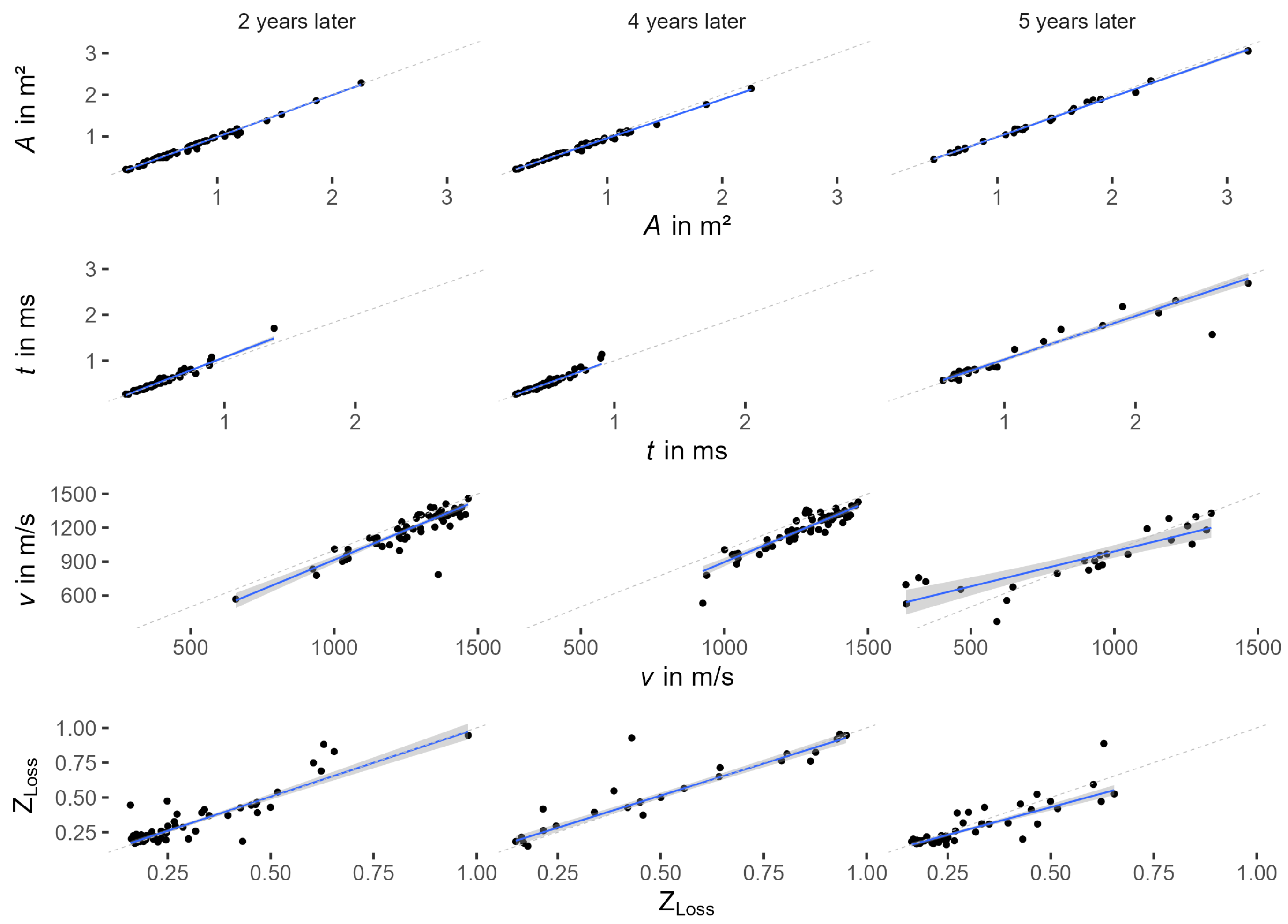
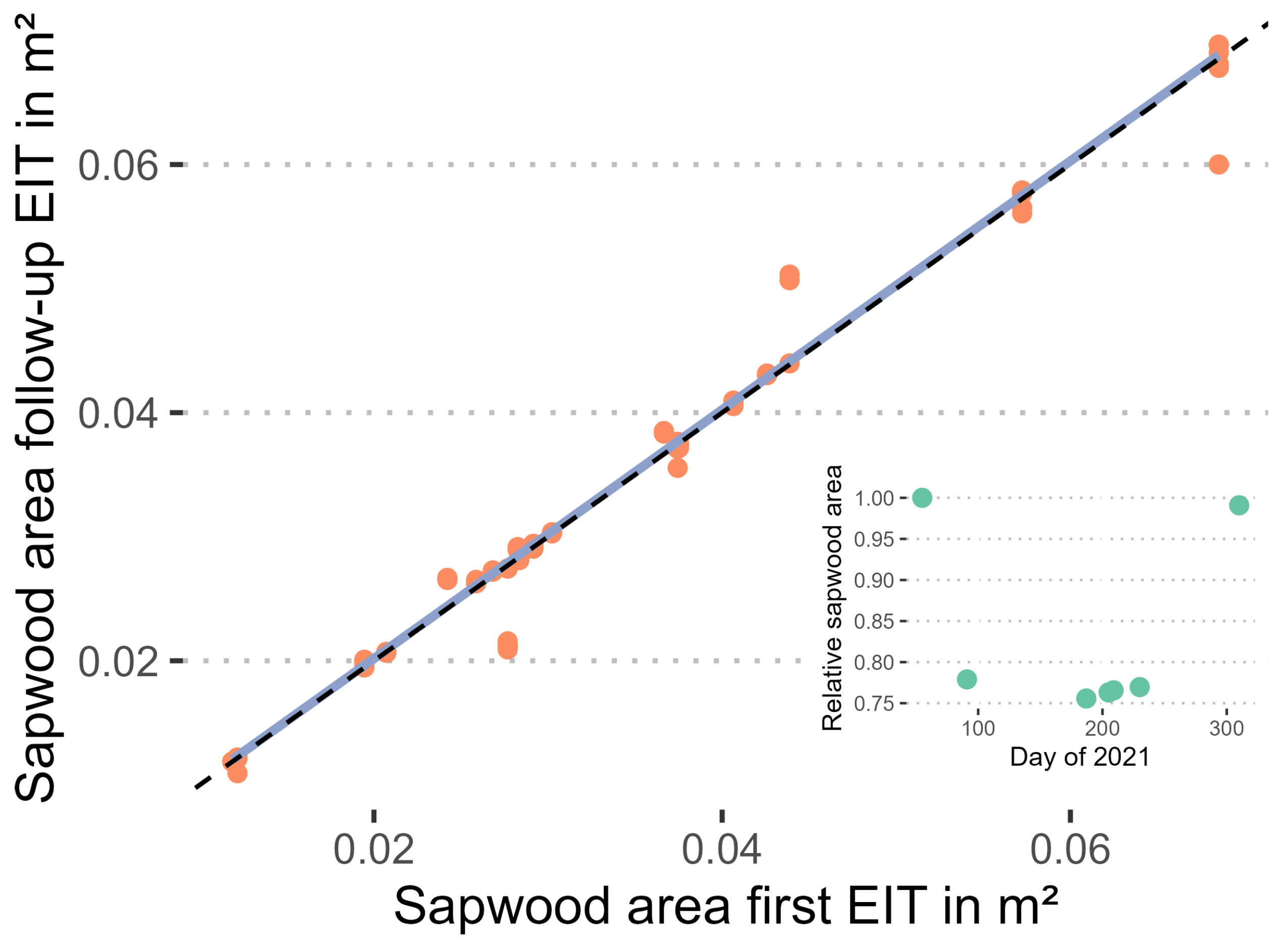
This study analyzed tomograms repeated within minutes or after several years, by the same or different operators, using either the same or a different experimental setup varying the sensor positions or the tomograph.
Stress wave tomograms were comparable even when measured by different operators some years apart. Thus, they typically allow monitoring the progress of decay, especially when SoT and ERT are combined [
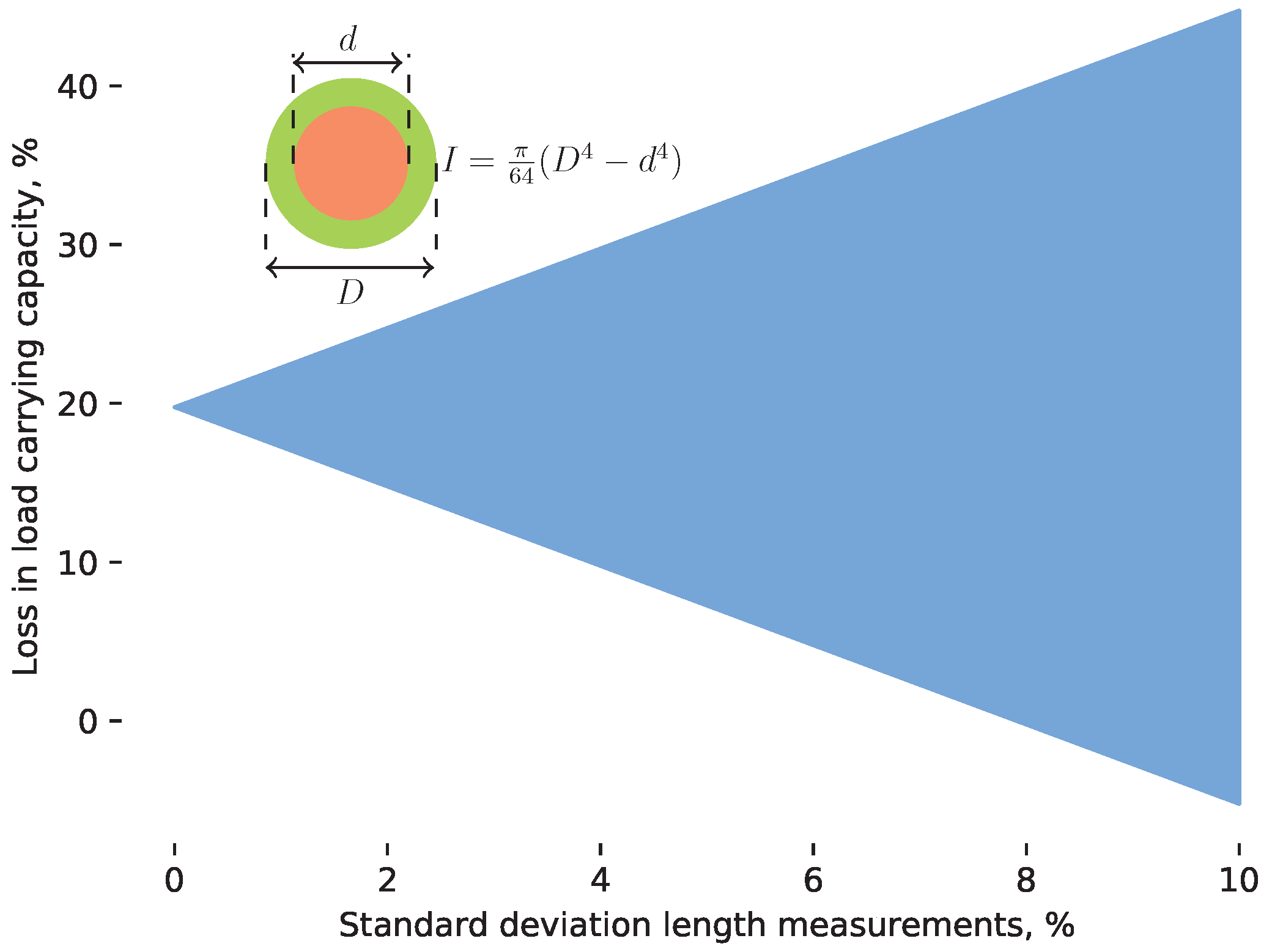
6]. In general, variation between repeated measurements increased with every computational step from raw data to tomograms, and was highest in parameters based on decayed area and section modulus. While measures of decayed area accumulate variation from time-of-flight, distance between sensors, and shape of the cross-section, loss of section modulus ( Z Loss ) is derived from the ratio of two parameters, accumulating all these sources of variation to the third power (Equations (1)–(4)). This propagation of variation is further illustrated in 
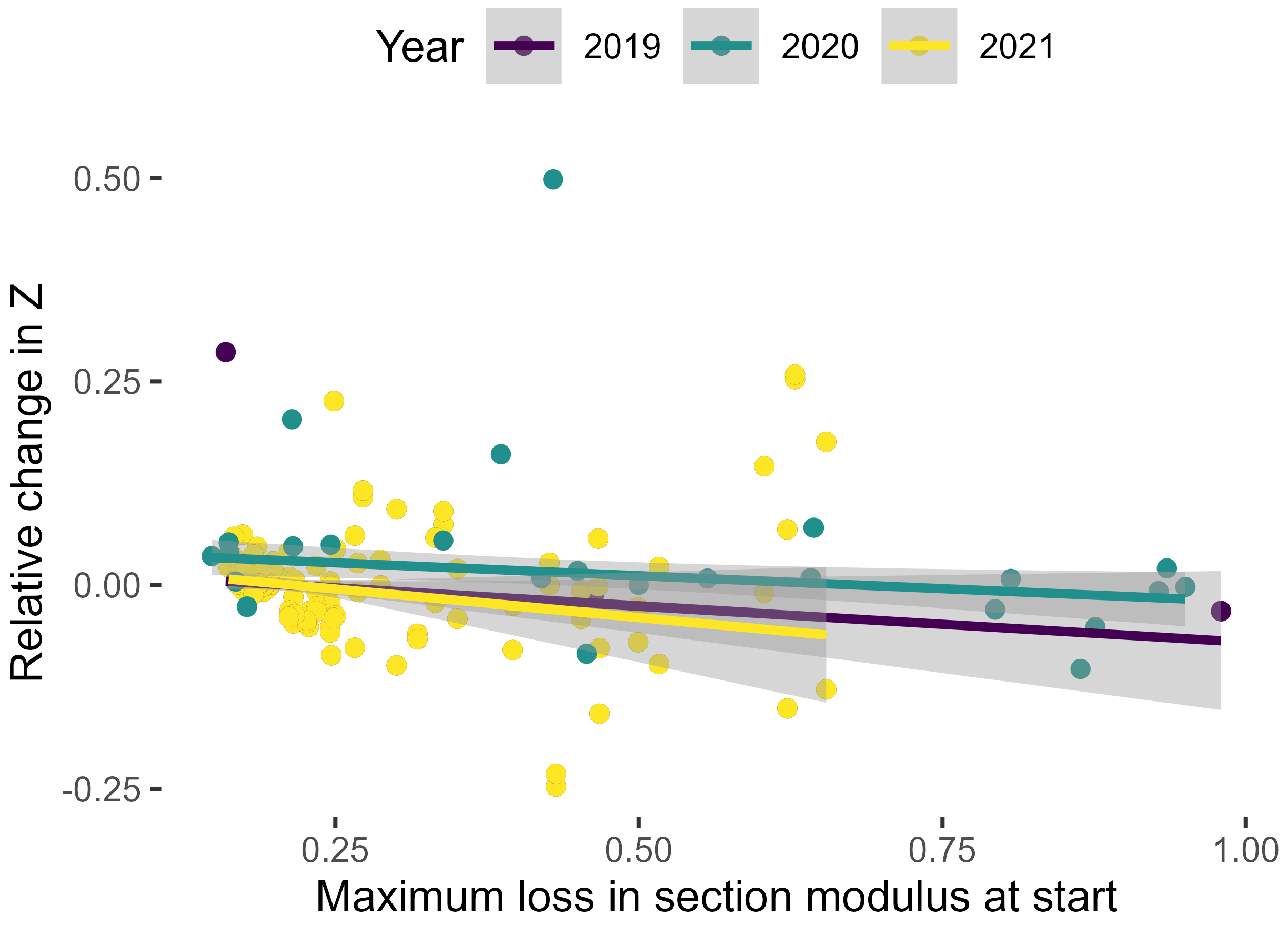
Figure 10. Even for a perfectly round tree with a perfectly round central cavity, length measurements with a standard deviation of 10% result in a standard deviation of 25% in Z Loss .
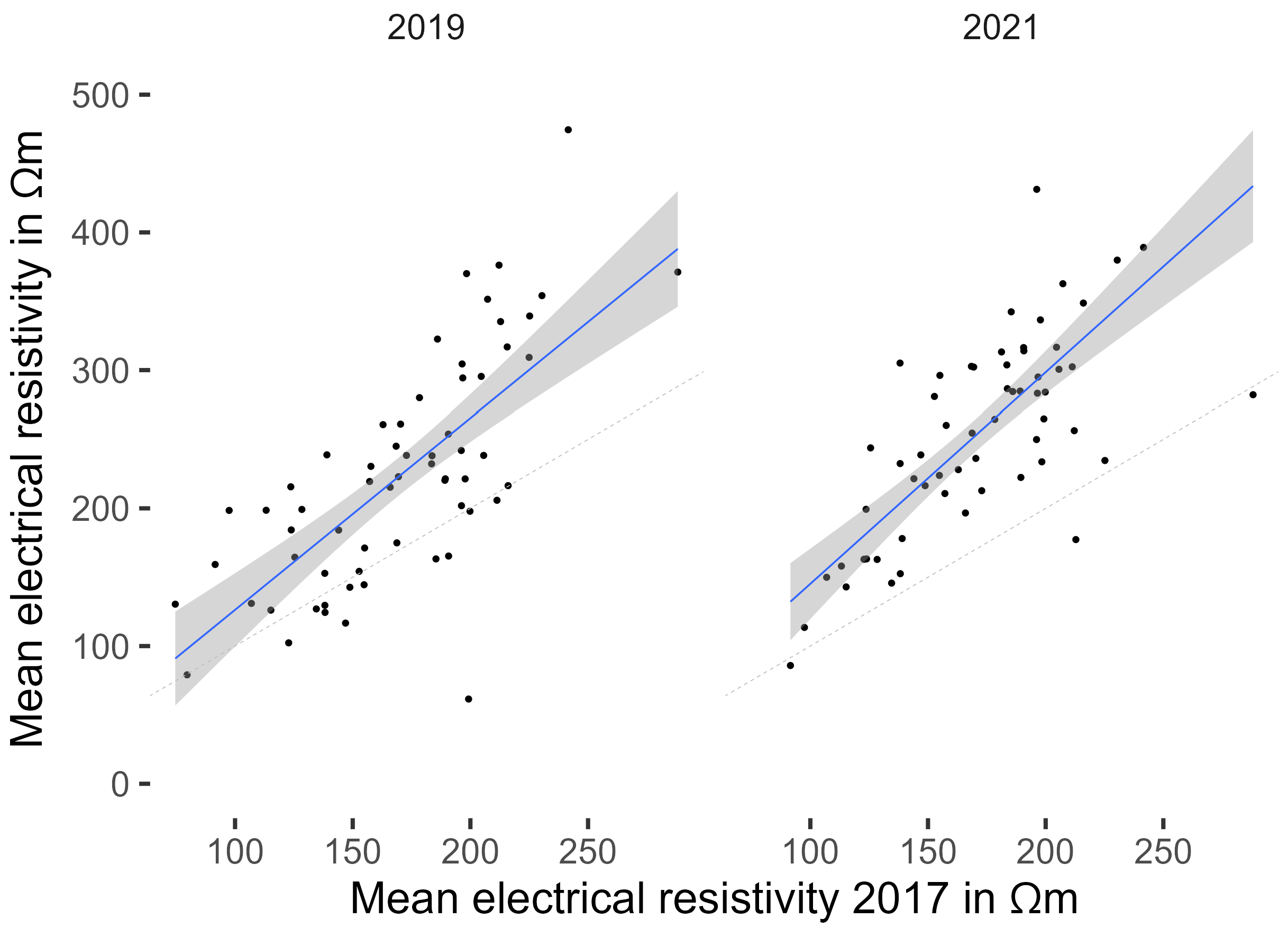
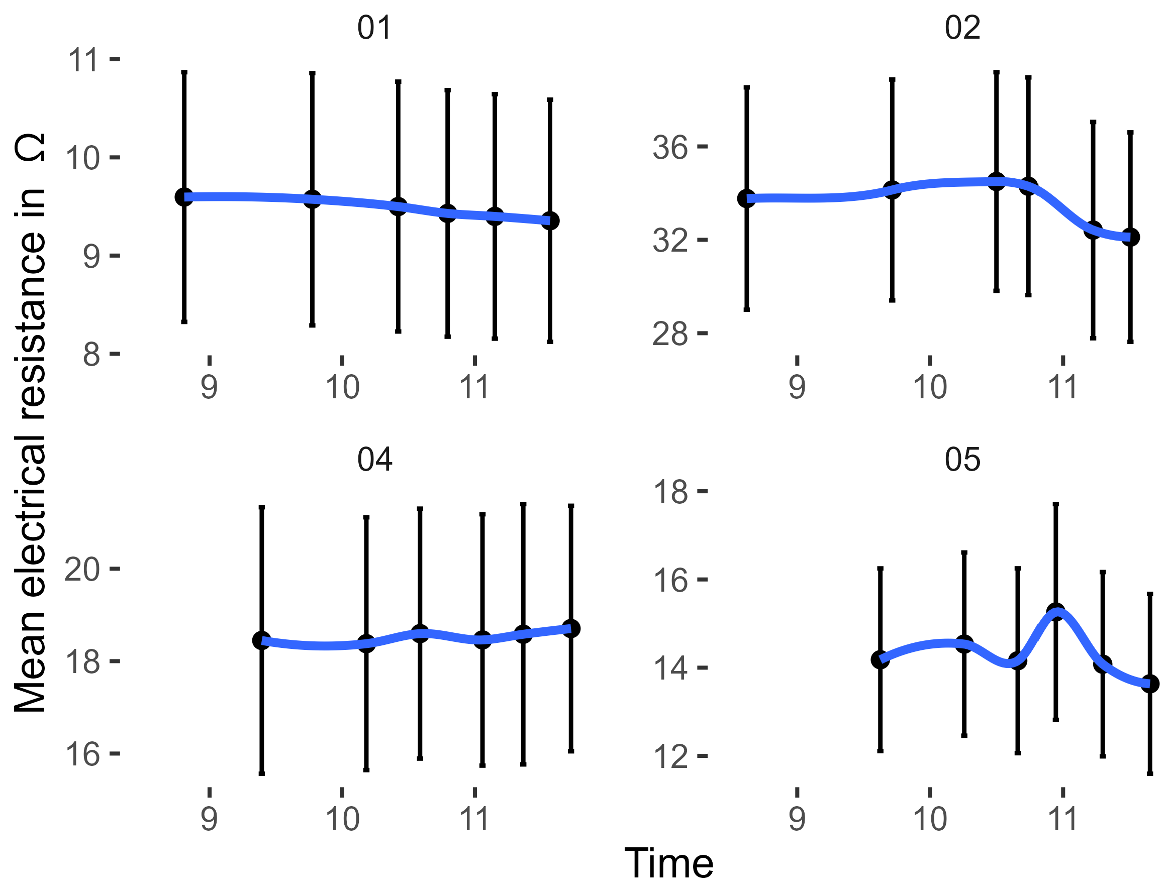
Between repeated measurements, the change in mean Z Loss per site ranged from −23% to +7%. Although overall, section modulus decreased with time as would be expected, especially, when the initial Z Loss was large, even large positive gains in section modulus were recorded after 5 years of advancing decay (Figure 11). Because trees cannot repair decay and diameter increment was very low in these old trees, some of these results must be wrong and illustrate the potential impact of apparently small variation of raw data on highly aggregated parameters like Z Loss .
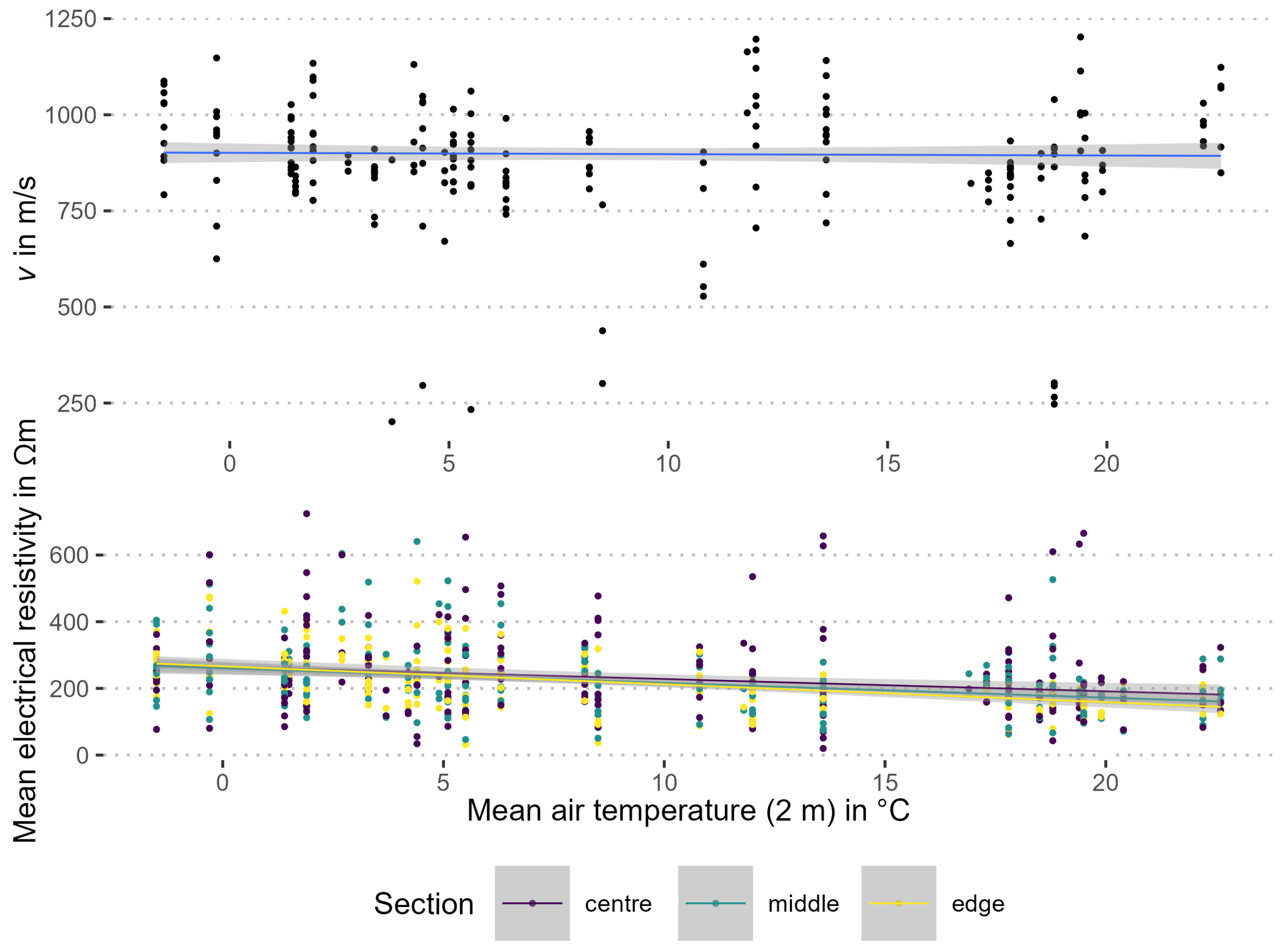
At temperatures above freezing, stress wave velocity is not statistically significantly affected by temperature change. This agrees with previous studies [14,16,36,37,38,39,40,41]. Only well below freezing, when the stem or parts of it are frozen, velocity increases and affects SoT [42]. And unlike ERT, SoT is very unlikely to be affected by changing wood moisture content, because reported variation of stress wave velocity above the fibre-saturation point is generally very low [15,40,41,43,44,45], especially when compared to effects of wood decay. Therefor, differences in wood moisture content and wood temperature are unlikely to have contributed to the variation in the tomograms.
It is likely that the main source of variation in SoT is the operator. When SoT was repeated immediately by different operators using the same or different nails and positions, v changed by up 5%. This was caused by differences in sensor distance d (≤1% change) and time-of-flight t (≤6% change). Sensor distance was measured manually with an electronic caliper and therefor varied between operators due to individual levels of accuracy. Time-of-flight t depends to a small degree on the force of excitation [46] and is also influenced by the individual operator. For the practical application of SoT in tree risk assessment is important to note that the end product of the method, the area of defects, was not significantly affected by the operator.
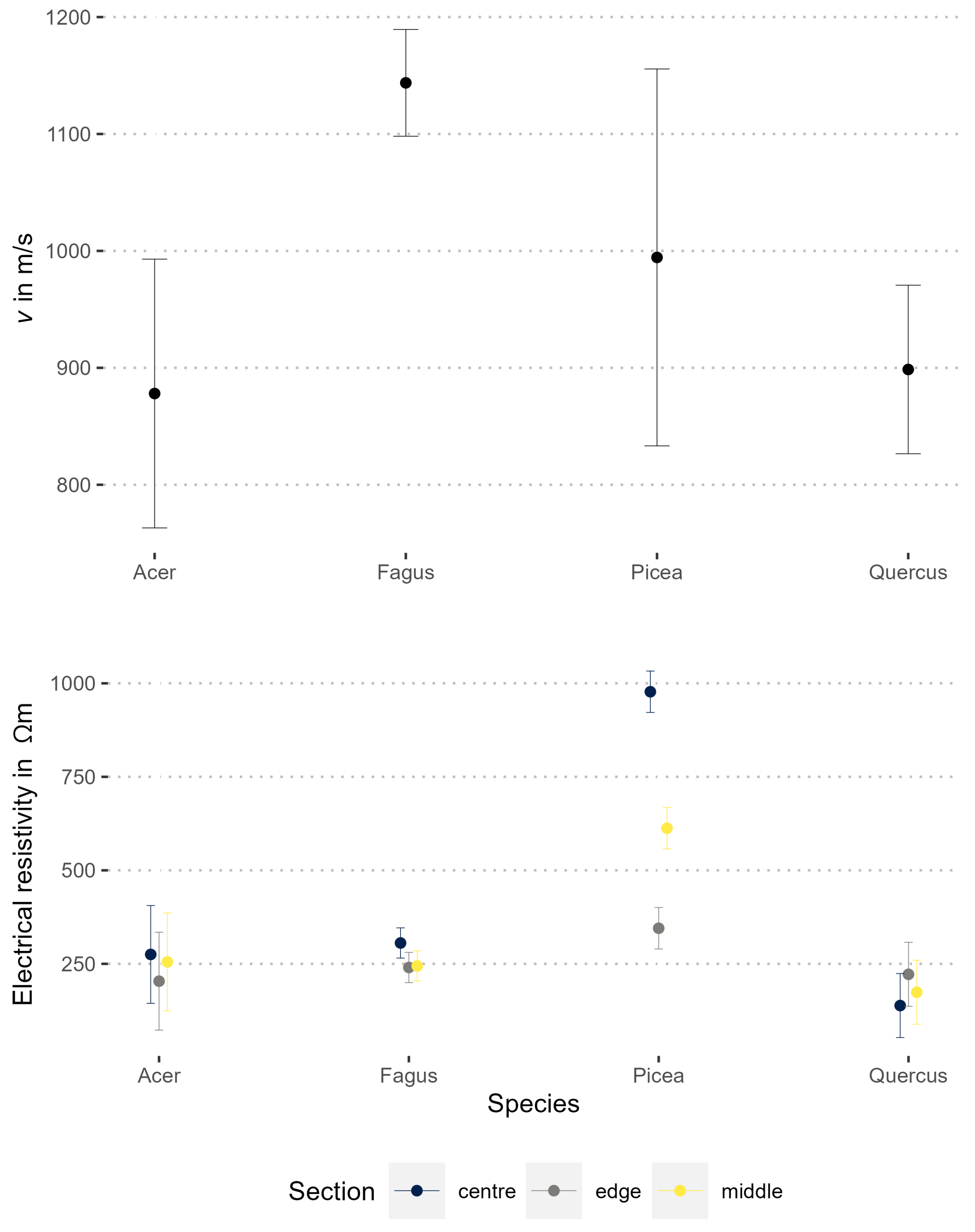
Stress-wave velocity v in beech was statistically significant higher than in the other species ( p < 0.0001 ), which did not differ from each other. Most trees had decay, cavities, and cracks in their stems, so that these data might not be representative for the species.
ρ and ERT based on it were less repeatable than v and SoT. Most likely, varying wood moisture and temperature contributed to this difference. Temperature changes affected ρ well above 0 °C (Figure 5), as has already been reported in earlier studies [17,18,35,47,48,49]. Changing irradiation on the stem, and changing stem and sap temperatures, can all cause variability in ρ at the stem surface and in sap wood. Changes in stem water content during transpiration are a further source of variation [33], although they are unlikely to affect tomograms of urban trees visibly. Ref. [19] reported 5% variation in the resistivity between successive measurements, somewhat more than the 2% found in the present study. However, centering the data of each tomogram before further processing [50] eliminated the correlation with temperature completely (data not shown) and is highly recommended when comparing ERT over time.
In spruce, dry heartwood contributed significantly to variation in ρ . This is typical for many temperate conifer species and has been used to measure heartwood area [3,51,52]. ρ of the hardwood species in this study was rather homogeneous.
It is important to note, that it is inherent to the process of inversion that the absolute values assigned to a triangle of the mesh are affected by the choice of parameters and thus are less stable than the ratios between all values assigned to the mesh. Lastly, changes in ERT often indicate advancing decay and tend to precede changes in SoT. Thus, they should not be treated as error without further investigation.
The small but significant effects of temperature on ERT that are reported here and have been shown in earlier studies [17,18,35,47,48,49], although relevant for scientific applications of ERT, affected resulting tomograms only marginally. Thus, ERT can be applied by tree assessors together with SoT, as long as temperatures are well above freezing.
Contrary to findings by [17], long-term installation in P. abies did not affect ER tomograms.
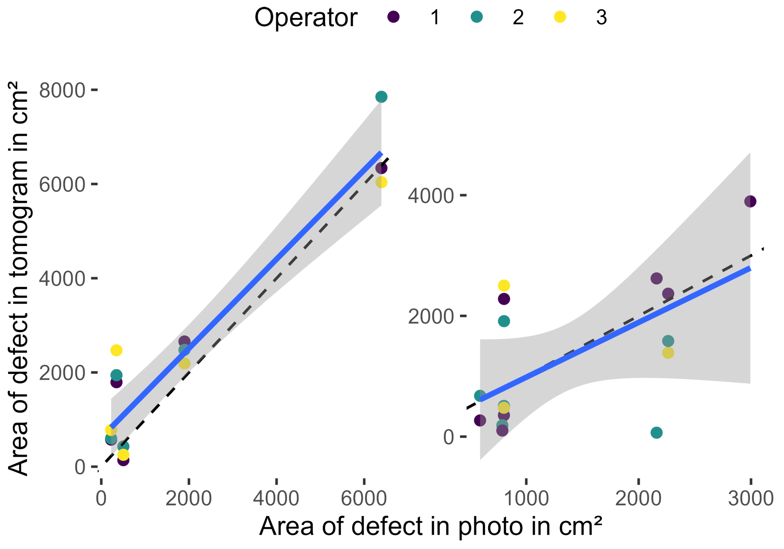
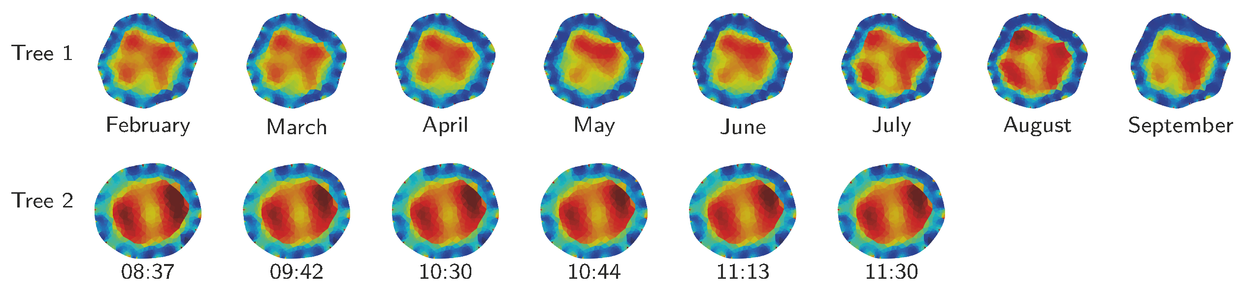
Assessing the quality of tomograms by comparing them to photographic images has proven difficult. Without the assistance of other devices, in this study a penetrometer, the visual delineation of decay in the image is error-prone, as is the necessarily somewhat arbitrary color threshold in the tomogram used to estimate Z Loss .
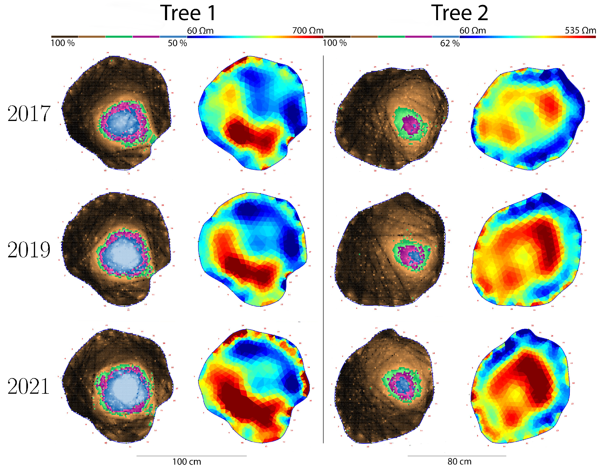
Judged by the tomograms, the spread of decay after 2 to 5 years was low for most trees. While the progress of decay has been extensively studied in vitro [53], much less is known about the speed at which fungi decay standing urban trees [54], so these results at least indicate a time-frame for follow-up measurements for tree risk assessment. Tomography, and especially the combination of SoT and ERT, is an excellent tool for further non-destructive studies in this field. They would supply tree assessors with much-needed information to decide on the intervals between successive advanced tree assessments.
As long as wood is not frozen, large differences in stem surface temperature are absent (for ERT), sensor positions are recorded and documented precisely, and previous sensor positions are re-used, results of follow-up measurements can safely be interpreted in terms of progress of decay. Although changing sensor positions should in theory not affect tomograms, it will complicate the interpretation of differences between measurements. When repeating a measurement, tree assessors should therefor try to use the same sensor positions whenever possible. Complex derived parameters like loss of load bearing capacity Z Loss should be interpreted with great caution, because of their amplified uncertainty.
Within these limitations, results should increase confidence in tomographic measurements.

Funding

This research received no external funding.

Data Availability Statement

Data are not publicly available due to legal and privacy issues.

Acknowledgments

The cities of Hannover and Göttingen, as well as the Forest Cooperative Geismar made this study possible by providing access to trees. Several students provided data measured under the supervision of the author.

Conflicts of Interest

The author declares no conflict of interest.

Abbreviations

The following abbreviations are used in this manuscript:
ACross-sectional area, m2
ddistance
ERTElectrical resistivity tomography
ρ Electrical resistivity, Ωm
SoTStress wave tomography
tStress wave travel-time, time-of-flight
vStress wave velocity, m s−1
ZSection modulus, m3
Z Loss Loss of section modulus

Appendix A

Summaries of statistical analyses. Model estimates and 95% confidence intervals. Significant effects are indicated by asterisks: *** p < 0.01 ; ** p < 0.05 ; * p < 0.1 .
Table A1. Statistical analysis of data presented in Figure 2.
CSA 2021
Generalized Least Squares
CSA 20170.928 *** (0.907, 0.948)
Constant0.023 *** (0.006, 0.040)
N54
Table A2. Statistical analysis of data presented in Figure 2.
CSA 2020
Generalized Least Squares
CSA 20150.970 *** (0.946, 0.995)
Constant0.015 (−0.011, 0.041)
N29
Table A3. Statistical analysis of data presented in Figure 2.
Time-of-Flight
Linear Mixed Effects
Year 20190.0001 *** (0.00004, 0.0001)
Year 20210.0001 *** (0.0001, 0.0001)
d0.001 *** (0.001, 0.001)
Year 2019:d0.0002 *** (0.0002, 0.0003)
Year 2021:d0.0002 *** (0.0002, 0.0003)
Constant0.001 *** (0.001, 0.001)
N52,685
Table A4. Statistical analysis of data presented in Figure 2.
Time-of-Flight
Linear Mixed Effects
Year 2020−0.00004 ** (−0.0001, −0.00000)
d0.002 *** (0.001, 0.002)
Year 2020:d−0.0004 *** (−0.0005, −0.0003)
Constant0.001 *** (0.001, 0.001)
N15,034
Table A5. Statistical analysis of data presented in Figure 2.
Velocity
Linear Mixed Effects
Year 2019−83.843 *** (−90.023, −77.663)
Year 2021−82.239 *** (−88.714, −75.764)
d385.596 *** (371.721, 399.472)
Year 2019:d−116.463 *** (−134.705, −98.221)
Year 2021:d−143.544 *** (−162.900, −124.187)
Constant1196.230 *** (1153.759, 1238.701)
N52,685
Table A6. Statistical analysis of data presented in Figure 2.
Velocity
Linear Mixed Effects
d−288.695 *** (−308.006, −269.384)
Year 2020−77.531 *** (−104.349, −50.713)
d:Year 202061.460 *** (36.516, 86.404)
Constant1178.768 *** (1087.910, 1269.626)
N10,017
Table A7. Statistical analysis of data presented in Figure 2.
Z Loss
Linear Mixed Effects
Constant0.344 *** (0.298, 0.389)
N204
Table A8. Statistical analysis of data presented in Figure 2.
Z Loss
Linear Mixed Effects
Year0.008 (−0.001, 0.017)
Constant−15.038 (−33.223, 3.148)
N51
Table A9. Statistical analysis of data presented in Figure 3.
Decay in Tomogram
Linear Mixed Effects
Operator 2360.228 (−260.478, 980.935)
Operator 345.803 (−574.904, 666.509)
Site PA1042.200 (−236.794, 2321.193)
Operator 2:Site PA−1179.744 (−2737.216, 377.729)
Operator 3:Site PA−543.753 (−2621.287, 1533.780)
Constant1962.491 ** (159.324, 3765.658)
N33
Table A10. Statistical analysis of data presented in Figure 4.
Velocity
Linear Mixed Effects
Species Fagus101.765 (−27.576, 231.106)
Species Picea−6.438 (−212.318, 199.443)
Species Quercus75.431 (−66.245, 217.107)
d5.746 (−42.482, 53.975)
Species Fagus:d254.883 *** (205.903, 303.862)
Species Picea:d188.407 *** (124.049, 252.765)
Species Quercus:d−73.114 *** (−123.187, −23.040)
Constant873.880 *** (753.399, 994.362)
N68,451
Table A11. Statistical analysis of data presented in Figure 4.
R
Linear Mixed Effects
Species Fagus30.617 (−106.249, 167.482)
Species Picea702.369 *** (560.373, 844.365)
Species Quercus−136.691 * (−292.989, 19.606)
Section edge−71.491 (−210.607, 67.624)
Section middle−19.997 (−159.113, 119.119)
Species Fagus:Section edge6.014 (−136.829, 148.857)
Species Picea:Section edge−560.837 *** (−711.898, −409.776)
Species Quercus:Section edge154.985 * (−11.290, 321.260)
Species Fagus:Section middle−41.345 (−184.188, 101.498)
Species Picea:Section middle−344.959 *** (−496.020, −193.898)
Species Quercus:Section middle55.538 (−110.737, 221.813)
Constant275.118 *** (144.350, 405.885)
N984
Table A12. Statistical analysis of data presented in Figure 5.
Velocity
Linear Mixed Effects
Air temperature−0.678 * (−1.422, 0.066)
Constant900.022 *** (870.669, 929.376)
N215
Table A13. Statistical analysis of data presented in Figure 5.
R
Linear Mixed Effects
Section middle19.333 *** (7.814, 30.851)
Section edge21.844 *** (10.325, 33.364)
Air temperature−3.072 *** (−3.741, −2.403)
Section middle:Air temperature−0.864 * (−1.764, 0.036)
Section edge:Air temperature−1.552 *** (−2.452, −0.652)
Constant248.454 *** (229.677, 267.231)
N648
Table A14. Statistical analysis of data presented in Figure 7.
R
Linear Mixed Effects
Section middle19.333 *** (7.814, 30.851)
Section edge21.844 *** (10.325, 33.364)
Air temperature−3.072 *** (−3.741, −2.403)
Section middle:Air temperature−0.864 * (−1.764, 0.036)
Section edge:Air temperature−1.552 *** (−2.452, −0.652)
Constant248.454 *** (229.677, 267.231)
N648
Table A15. Statistical analysis of data presented in Figure 8.
R
Linear Mixed Effects
Repetition 2−0.066 (−0.211, 0.078)
Repetition 30.234 *** (0.089, 0.378)
Repetition 40.552 *** (0.408, 0.697)
Repetition 50.814 *** (0.670, 0.959)
Repetition 61.000 *** (0.855, 1.144)
Constant−49.086 *** (−63.570, −34.602)
N5148
Table A16. Statistical analysis of data presented in Figure 9.
Sap Wood Area
Linear Mixed Effects
Tag0.00000 (−0.00000, 0.00000)
Constant0.033 *** (0.026, 0.039)
N96
Table A17. Statistical analysis of data presented in Figure 11.
Decay in Tomogram
Linear Mixed Effects
Operator 2360.228 (−260.478, 980.935)
Operator 345.803 (−574.904, 666.509)
Site PA1042.200 (−236.794, 2321.193)
Operator 2:Site PA−1179.744 (−2737.216, 377.729)
Operator 3:Site PA−543.753 (−2621.287, 1533.780)
Constant1962.491 ** (159.324, 3765.658)
N33

References

  1. Rust, S. A new tomographic device for the non-destructive testing of standing trees. In Proceedings of the 12th International Symposium on Nondestructive Testing of Wood, Sopron, Hungary, 13–16 September 2000; pp. 233–238. [Google Scholar]
  2. Bieker, D.; Rust, S. Electric Resistivity Tomography Shows Radial Variation of Electrolytes in Quercus Robur. Can. J. For. Res. 2010, 40, 1189–1193. [Google Scholar] [CrossRef]
  3. Bieker, D.; Rust, S. Non-Destructive Estimation of Sapwood and Heartwood Width in Scots Pine (Pinus Sylvestris L.). Silva Fenn. 2010, 44, 267–273. [Google Scholar] [CrossRef] [Green Version]
  4. Bieker, D.; Kehr, R.; Weber, G.; Rust, S. Non-Destructive Monitoring of Early Stages of White Rot by Trametes Versicolor in Fraxinus Excelsior. Ann. For. Sci. 2010, 67, 210. [Google Scholar] [CrossRef] [Green Version]
  5. Bär, A.; Hamacher, M.; Ganthaler, A.; Losso, A.; Mayr, S. Electrical Resistivity Tomography: Patterns in Betula Pendula, Fagus Sylvatica, Picea Abies and Pinus Sylvestris. Tree Physiol. 2019, 39, 1262–1271. [Google Scholar] [CrossRef] [PubMed]
  6. Rust, S.; Göcke, L.; Weihs, U.; Günther, T.; Rücker, C. Combining Sonic and Electric Impedance Tomography for Nondestructive Testing of Trees. In Proceedings of the 15th International Symposium on Nondestructive Testing of Wood, Madison, WI, USA, 10–12 September 2007; Forest Products Society: Duluth, MN, USA, 2007. [Google Scholar]
  7. Mattheck, C.; Bethge, K.; West, P.W. Breakage of Hollow Tree Stems. Trees-Struct. Funct. 1994, 9, 47–50. [Google Scholar] [CrossRef]
  8. Kane, B.; Ryan, D.; Bloniarz, D.V. Comparing Formulae That Assess Strength Loss Due to Decay in Trees. J. Arboric. 2001, 27, 78–87. [Google Scholar]
  9. Burcham, D.C.; Brazee, N.J.; Marra, R.E.; Kane, B. Can Sonic Tomography Predict Loss in Load-Bearing Capacity for Trees with Internal Defects? A Comparison of Sonic Tomograms with Destructive Measurements. Trees 2019, 33, 681–695. [Google Scholar] [CrossRef]
  10. Ciftci, C.; Kane, B.; Brena, S.F.; Arwade, S.R. Loss in Moment Capacity of Tree Stems Induced by Decay. Trees 2014, 28, 517–529. [Google Scholar] [CrossRef]
  11. Rust, S. Accuracy and Reproducibility of Acoustic Tomography Significantly Increase with Precision of Sensor Position. J. For. Landsc. Res. 2017, 2, 1–6. [Google Scholar] [CrossRef]
  12. Newton, P.F. Quantifying the Effects of Wood Moisture and Temperature Variation on Time-of-Flight Acoustic Velocity Measures within Standing Red Pine and Jack Pine Trees. Forests 2018, 9, 527. [Google Scholar] [CrossRef] [Green Version]
  13. Llana, D.F.; Iniguez-Gonzalez, G.; Martinez, R.D.; Arriaga, F. Influence of Timber Moisture Content on Wave Time-of-Flight and Longitudinal Natural Frequency in Coniferous Species for Different Instruments. Holzforschung 2018, 72, 405–411. [Google Scholar] [CrossRef]
  14. Gao, S.; Tao, X.; Wang, X.; Wang, L. Theoretical Modeling of the Effects of Temperature and Moisture Content on the Acoustic Velocity of Pinus Resinosa Wood. J. For. Res. 2018, 29, 541–548. [Google Scholar] [CrossRef]
  15. Cristini, V.; Tippner, J.; Vojáčková, B.; Paulić, V. Comparison of Variability in Results of Acoustic Tomographs in Pedunculate Oak (Quercus Robur L.). BioResources 2021, 16, 3046–3058. [Google Scholar] [CrossRef]
  16. Gao, S.; Wang, X.; Wang, L.; Allison, R.B. Effect of Temperature on Acoustic Evaluation of Standing Trees and Logs: Part 2: Field Investigation. Wood Fiber Sci. 2013, 45, 15–25. [Google Scholar]
  17. Ganthaler, A.; Sailer, J.; Bär, A.; Losso, A.; Mayr, S. Noninvasive Analysis of Tree Stems by Electrical Resistivity Tomography: Unraveling the Effects of Temperature, Water Status, and Electrode Installation. Front. Plant Sci. 2019, 10, 1455. [Google Scholar] [CrossRef]
  18. Yue, X.; Wang, L.; Shi, X.; Xu, M.; Zhu, Z. Investigations on the Effects of Seasonal Temperature Changes on the Electrical Resistance of Living Trees. Forests 2018, 9, 550. [Google Scholar] [CrossRef] [Green Version]
  19. Hanskötter, B. Diagnose Fakultativer Farbkerne an Stehender Rotbuche (Fagussylvatica L.) Mittels Elektrischer Widerstandstomographie. Ph.D. Thesis, Georg-August-Universität Göttingen, Fakultät für Forstwissenschaften und Waldökologie, Göttingen, Germany, 2004. [Google Scholar]
  20. Günther, T.; Rücker, C.; Spitzer, K. Three-Dimensional Modelling and Inversion of Dc Resistivity Data Incorporating Topography—II. Inversion. Geophys. J. Int. 2006, 166, 506–517. [Google Scholar] [CrossRef] [Green Version]
  21. Rücker, C.; Günther, T.; Spitzer, K. Three-Dimensional Modelling and Inversion of Dc Resistivity Data Incorporating Topography—I. Modelling. Geophys. J. Int. 2006, 166, 495–505. [Google Scholar] [CrossRef] [Green Version]
  22. Son, J.; Kim, S.; Shin, J.; Lee, G.; Kim, H. Reliability of Non-Destructive Sonic Tomography for Detection of Defects in Old ZelkovaSerrata (Thunb.) Makino Trees. For. Sci. Technol. 2021, 17, 110–118. [Google Scholar] [CrossRef]
  23. DWD. Climate Data Center. Available online: https://cdc.dwd.de/portal/ (accessed on 30 December 2021).
  24. Koizumi, A.; Hirai, T.; H, T. Evaluation of the Section Modulus for Tree-Stem Cross Sections of Irregular Shape. J. Wood Sci. 2006, 52, 213–219. [Google Scholar] [CrossRef] [Green Version]
  25. Doube, M.; Kłosowski, M.M.; Arganda-Carreras, I.; Cordelières, F.P.; Dougherty, R.P.; Jackson, J.S.; Schmid, B.; Hutchinson, J.R.; Shefelbine, S.J. BoneJ: Free and Extensible Bone Image Analysis in ImageJ. Bone 2010, 47, 1076–1079. [Google Scholar] [CrossRef] [PubMed] [Green Version]
  26. Schindelin, J.; Arganda-Carreras, I.; Frise, E.; Kaynig, V.; Longair, M.; Pietzsch, T.; Preibisch, S.; Rueden, C.; Saalfeld, S.; Schmid, B.; et al. Fiji: An Open-Source Platform for Biological-Image Analysis. Nat. Methods 2012, 9, 676–682. [Google Scholar] [CrossRef] [PubMed] [Green Version]
  27. Domander, R.; Felder, A.A.; Doube, M. BoneJ2—Refactoring Established Research Software. Wellcome Open Res. 2021, 6, 37. [Google Scholar] [CrossRef] [PubMed]
  28. R Core Team. R: A Language and Environment for Statistical Computing; R Foundation for Statistical Computing: Vienna, Austria, 2021. [Google Scholar]
  29. Pinheiro, J.; Bates, D.; DebRoy, S.; Sarkar, D.; R. Core Team. Nlme: Linear and Nonlinear Mixed Effects Models. 2022. Available online: https://cran.r-project.org/web/packages/nlme/nlme.pdf (accessed on 30 December 2021).
  30. Pinheiro, J.C.; Bates, D.M. Mixed-Effects Models in S and S-PLUS; Statistics and Computing; Springer: New York, NY, USA; Berlin/Heidelberg, Germany, 2004. [Google Scholar]
  31. Wilcox, R.R. Introduction to Robust Estimation and Hypothesis Testing; Elsevier Science & Technology Books: San Diego, CA, USA, 2011. [Google Scholar]
  32. Martin, L.; Cochard, H.; Mayr, S.; Badel, E. Using Electrical Resistivity Tomography to Detect Wetwood and Estimate Moisture Content in Silver Fir (Abies Alba Mill.). Ann. For. Sci. 2021, 78, 65. [Google Scholar] [CrossRef]
  33. Losso, A.; Sailer, J.; Bär, A.; Ganthaler, A.; Mayr, S. Insights into Trunks of Pinus Cembra L.: Analyses of Hydraulics via Electrical Resistivity Tomography. Trees 2020, 34, 999–1008. [Google Scholar] [CrossRef] [PubMed]
  34. Deflorio, G.; Fink, S.; Schwarze, F.W.M.R. Detection of Incipient Decay in Tree Stems with Sonic Tomography after Wounding and Fungal Inoculation. Wood Sci. Technol. 2008, 42, 117–132. [Google Scholar] [CrossRef]
  35. Mares, R.; Barnard, H.R.; Mao, D.; Revil, A.; Singha, K. Examining Diel Patterns of Soil and Xylem Moisture Using Electrical Resistivity Imaging. J. Hydrol. 2016, 536, 327–338. [Google Scholar] [CrossRef] [Green Version]
  36. Gao, S.; Wang, X.; Wang, L.; Allison, R.B. Effect of Temperature on Acoustic Evaluation of Standing Trees and Logs: Part 1-Laboratory Investigation. Wood Fiber Sci. 2012, 44, 286–297. [Google Scholar]
  37. Gao, S.; Wang, X.; Wang, L. Modeling Temperature Effect on Dynamic Modulus of Elasticity of Red Pine (PinusResinosa) in Frozen and Non-Frozen States. Holzforschung 2015, 69, 233–240. [Google Scholar] [CrossRef]
  38. Gao, S.; Wang, X.; Wang, L.; Bruce, R.B. Modeling Temperature and Moisture State Effects on Acoustic Velocity in Wood. In Proceedings of the 17th International Nondestructive Testing and Evaluation of Wood Symposium, Sopron, Hungary, 14–16 September 2011; pp. 411–418. [Google Scholar]
  39. Baechle, H.; Walker, J. The Influence of Temperature on the Velocity of Sound in Green Pine Wood. Holz als Roh-und Werkst. 2006, 64, 429–430. [Google Scholar] [CrossRef]
  40. Kang, H.; Booker, R.E. Variation of Stress Wave Velocity with MC and Temperature. Wood Sci. Technol. 2002, 36, 41–54. [Google Scholar] [CrossRef]
  41. Llana, D.F.; Iniguez-Gonzalez, G.; Arriaga, F.; Niemz, P. Influence of Temperature and Moisture Content on Non-Destructive Measurements in Scots Pine Wood. Wood Res. 2014, 59, 769–780. [Google Scholar]
  42. Rust, S. Baumdiagnose bei Frost. Grünforum LA 2003, 33, 36–38. [Google Scholar]
  43. Minamisawa, A.; Ozawa, A.; Sakai, H.; Takagi, K. Moisture effects on the ultrasonic velocities in woods. In Proceedings of the IEEE Symposium on Ultrasonics, Honolulu, HI, USA, 4–7 December 1990. [Google Scholar] [CrossRef]
  44. Llana, D.F.; Short, I.; Harte, A.M. Use of Non-Destructive Test Methods on Irish Hardwood Standing Trees and Small-Diameter Round Timber for Prediction of Mechanical Properties. Ann. For. Sci. 2020, 77, 62. [Google Scholar] [CrossRef]
  45. Llana, D.F.; Iniguez-Gonzalez, G.; Esteban, M.; Hermoso, E.; Arriaga, F. Timber Moisture Content Adjustment Factors for Nondestructive Testing (NDT): Acoustic, Vibration and Probing Techniques. Holzforschung 2020, 74, 817–827. [Google Scholar] [CrossRef]
  46. Aurich, M. Einfluss der Klopfstärke auf die Schalltomographie. BSc Thesis, University of Applied Science and Arts, Göttingen, Germany, 2017. [Google Scholar]
  47. Nursultanov, N.; Altaner, C.; Heffernan, W.J.B. Effect of Temperature on Electrical Conductivity of Green Sapwood of Pinus Radiata (Radiata Pine). Wood Sci. Technol. 2017, 51, 795–809. [Google Scholar] [CrossRef]
  48. Luo, Z.; Guan, H.; Zhang, X. The Temperature Effect and Correction Models for Using Electrical Resistivity to Estimate Wood Moisture Variations. J. Hydrol. 2019, 578, 124022. [Google Scholar] [CrossRef]
  49. Nursultanov, N.; Heffernan, W.J.B.; Altaner, C.; Pang, S. Anisotropic Electrical Conductivity of Green Timber within 20–90 Degrees C Temperature Range. Wood Sci. Technol. 2020, 54, 1181–1196. [Google Scholar] [CrossRef]
  50. Rathai, R.S.; Rust, S. Über den Einfluss von Baumschnittmaßnahmen. AFZ-Der Wald 2013, 68, 35–36. [Google Scholar]
  51. Guyot, A.; Ostergaard, K.T.; Lenkopane, M.; Fan, J.; Lockington, D.A. Using Electrical Resistivity Tomography to Differentiate Sapwood from Heartwood: Application to Conifers. Tree Physiol. 2013, 33, 187–194. [Google Scholar] [CrossRef] [Green Version]
  52. Lin, C.J.; Chung, C.H.; Yang, T.H.; Lin, F.C. Detection of Electric Resistivity Tomography and Evaluation of the Sapwood-Heartwood Demarcation in Three Asia Gymnosperm Species. Silva Fenn. 2012, 46, 415–424. [Google Scholar] [CrossRef] [Green Version]
  53. Schwarze, F.W.M.R. Entwicklung und biomechanische Auswirkungen von holzzersetzenden Pilzen in lebenden Bäumen und in Vitro. Ph.D. Thesis, Universität Freiburg, Freiburg, Germany, 1995. [Google Scholar]
  54. Deflorio, G.; Johnson, C.; Fink, S.; Schwarze, F.W.M.R. Decay Development in Living Sapwood of Coniferous and Deciduous Trees Inoculated with Six Wood Decay Fungi. For. Ecol. Manag. 2008, 255, 2373–2383. [Google Scholar] [CrossRef]
Figure 1. SoT (1. and 3. column) and ERT (2. and 4. column) of two beech trees measured three times by different operators using slightly different sensor positions every time (site KF).
Forests 13 00295 g001
Figure 2. Correlation of initial and follow-up measurement of t, A, v and Z Loss . Tomography was repeated after 2 and 4 years at site KF and after 5 years at site TG. Dashed line indicates 1:1. Gray: 95% confidence interval.
Forests 13 00295 g002
Figure 3. Correlation of defect in tomograms and images of stem cross-sections (left: site PA2, operators used the same nails; right: site AP, operators used different nails at new locations). Dashed line indicates 1:1. Gray: 95% confidence interval.
Forests 13 00295 g003
Figure 4. Species differences in stress wave velocity (top) and electrical resistivity (bottom, area-weighted median). “centre” refers to the innermost third of the stem cross-section, “edge” to the outermost third, while “middle” refers to the remainder.
Forests 13 00295 g004
Figure 5. Correlation of tangential stress wave velocity (top), electrical resistivity ((bottom), area-weighted median), and air temperature (site KF). “centre” refers to the innermost third of the stem cross-section, “edge” to the outermost third, while “middle” refers to the remainder. Tomography was repeated for 4 years at site KF by different operators placing new sensor positions. Gray: 95% confidence interval.
Forests 13 00295 g005
Figure 6. ERT of two spruce trees measured several times in 2021 (top) and on one day in July (bottom), site PA1. Top row: every second measurement with Geotom, all else with Picus Treetronic.
Forests 13 00295 g006
Figure 7. Correlation of initial and follow-up measurement of ρ . Tomography was repeated after 2 (left), and 4 (right) years at site KF by different operators placing new sensor positions. Here, ρ is the area-weighted median of the outermost 33% of the stem cross-section. Dashed line indicates 1:1. Gray: 95% confidence interval.
Forests 13 00295 g007
Figure 8. Course of Ω from 8 o’clock until noon in four P. abies. Mean and standard error. Site PA1.
Forests 13 00295 g008
Figure 9. Sapwood area of 20 spruce trees measured several times in 2021 (site PA1, including only measurements with Picus TreeTronic). Inset shows variation of sapwood area in one individual tree with the largest changes in the sample. Blue: Linear Regression, gray: 95% confidence interval, dashed: 1:1.
Forests 13 00295 g009
Figure 10. Effect of variation in length measurements on the standard deviation of Z Loss (blue area). Assumptions: Diameter of cross-section D 1 m, diameter of cavity d 0.7 m. I: Second moment of area (Equation (2)).
Forests 13 00295 g010
Figure 11. Correlation of initial Z Loss and its changes at follow-up measurements. Tomography was repeated after 2 (2019), 5 (2020) and 4 (2021) years at sites TG and KF by different operators placing new sensor positions. Gray: 95% confidence interval.
Forests 13 00295 g011
Table 1. Sites, trees, and treatments.
SiteLocation 1TypeSpeciesnOperatorsDifferent NailsDifferent DevicesSeasonMeasurements
KFGöttingenopen fieldFagus sylvativa L.473x Sep. 2017, Sep.–Dec. 2019, Mar. 2021SoT, ERT
PA1GöttingenforestPicea abies (L.) Karst.201 xFeb.–Nov. 2021ERT
TGHannoverparkQuercus robur L.262x Oct. 2015, Oct. 2020SoT, ERT
APHeidelbergroadsideAcer pseudoplatanus L.53x May 2021SoT, ERT
PA2HeidelbergforestPicea abies (L.) Karst.73 Sep. 2014SoT
1 All sites in Germany.
Publisher’s Note: MDPI stays neutral with regard to jurisdictional claims in published maps and institutional affiliations.

