Improving the Accuracy of Estimating Forest Carbon Density Using the Tree Species Classification Method

Abstract

The accurate and effective estimation of forest carbon density is an essential basis for effectively responding to climate change and achieving the goal of carbon neutrality. Aiming at the problem of the significant differences in the forest carbon model parameters of different tree species, this study used the tree forest in Yueyang City, Hunan Province, China, as the study object and used the random forest classification algorithm through the Google Earth Engine platform to classify the dominant tree species within the forested range of the study area based on the image elements. The overall accuracy in the forest/non-forest classification (primary classification) was 93.79% with a Kappa of 0.9145. The overall accuracy in the dominant species classification (secondary classification) was 87.30% with a Kappa of 0.7747. Based on the classification, a multiple linear regression (MLR), support vector machine (SVM), and random forest (RF) were constructed for different dominant tree species by combining some Forest Resource Inventory data and remote sensing data. The results showed that the RF model had a significantly higher coefficient of determination (R² = 0.4054–0.7602) than the MLR (R² = 0.0900–0.4070) and SVM (R² = 0.1650–0.4450) as well as a substantially lower RMSE and MAE; its spatial distribution of forest carbon density ranged from 3.06 to 62.80 t·hm⁻². Compared with the spatial distribution of the forest carbon density (4.64 to 31.96 t·hm⁻²) without the classification of dominant species, the method eliminated the problems of severe overfitting and significant underestimation of peak values when estimating under unclassified conditions. The method provides a reference for the remote sensing inversion of forest carbon density on a large scale.

1. Introduction

Forests, the core of the global carbon cycle, are the largest aboveground carbon store in terrestrial ecosystems. Therefore, accurate estimation of forest carbon density based on image elements is crucial to understanding forests’ roles as atmospheric carbon sinks or sources. It is essential to effectively respond to climate change and achieve carbon neutrality targets [1,2,3,4,5].

The remote sensing inversion of forest carbon density will vary depending on the dominant tree species, topography, and other factors in the area of the survey sample size, resulting in different statistical relationships between field data and remote sensing factors. Some studies have also shown that the forest properties of other tree species vary greatly, so the remote sensing inversion of forest carbon density without a reasonable classification of tree species may result in significant differences in the inversion accuracy [6,7]. Therefore, this study proposed to prioritize the dominant tree species in the study area before conducting forest carbon density inversions to provide a forest carbon density estimation database. The primary studies on the use of remote sensing technology for forest species classification in recent years can be divided into: classification using a large amount of multispectral data with a low spatial resolution to compensate for the lack of spatial resolution by increasing the temporal resolution; classification using hyperspectral data based on the biochemical properties and leaf morphology of different forest tree species; classification of forest tree species based on high-spatial-resolution data using spectral information; and classification using LIDAR with differences in the vertical structure between different tree species. For example, Omer et al. [8] compared support vector machine (SVM) and artificial neural network (ANN) algorithms using WorldView-2 for the pixel-based classification of six tree species in a South African coastal forest. Meng, Y et al. [9] used a random forest classifier to classify tree species in remote sensing images based on terrain correction using an empirical rotation model. Currently, Landsat 8 OLI has a long-time-series feature that enables interannual observations at 30 m spatial resolution and is suitable for regional analysis. The Google Earth Engine (GEE) contains rich long-time-series remote sensing data and a robust cloud computing capability, which can improve the classification efficiency when classifying dominant tree species in large regions [10]. Therefore, this study used Landsat data and machine learning methods in the GEE to classify the dominant tree species in the forest range of the study area and to obtain a thematic map of the spatial distribution of the main dominant tree species in Yueyang City in order to provide a database for subsequent forest carbon density estimation.

In recent years, much research has been conducted on forest carbon density and change at different stand, regional, and national scales. Many methods have been developed to measure forest carbon density. These methods can be divided into several main categories: the forest biomass expansion factor method, micrometeorological methods, model simulation methods based on growth processes, and methods based on remote sensing estimates [11,12,13,14,15]. Among these, the traditional ground-based methods can provide accurate information. However, the time and labor required for extensive field surveys incur higher costs and makes them unavailable for the real-time mapping of carbon density over large areas. In contrast, methods based on remote sensing estimates are more comprehensive in time and space, have the advantage of being cost-effective, can dynamically invert forest carbon density over a region, and can monitor forest carbon density in a non-destructive manner. Remote-sensing-based estimation methods have become the most popular method for estimating forest carbon density. Various remote sensing sensors have been used to estimate forest carbon density; these can be divided into three categories: optical sensors, radar, and light detection and range (LiDAR) [16,17]. Optical sensors are mainly used to estimate forest carbon density based on their relationship with vegetation indices and texture image parameters of the forest floor; radar can provide information related to branches, trunks, and the forest floor to estimate forest carbon density using synthetic aperture radar; and LiDAR has specific advantages in terms of forest height and three-dimensional structure, which can be well obtained, but such data have not been widely used for the estimation of forest carbon density due to the expensive technology. Optical remote sensing data can provide rich canopy spectral and textural information for inversion modeling and is widely used for large-scale estimation of forest carbon density [18]. There are two models for estimating forest carbon density based on optical remote sensing: parametric and non-parametric models. Among these, the parametric models are mainly the linear regression model and partial-least-squares regression [19,20]. This model is simple and easy to construct but is based on the linear relationship between the forest carbon density and remote sensing variables for estimation. However, there are relatively complex relationships between remote sensing variables that are prone to problems such as multicollinearity, resulting in significant errors in the prediction of forest carbon density. Non-parametric models such as random forest, k-nearest neighbor, support vector machine, and artificial neural network algorithms can solve the non-linear correlation problem in inversion [21,22,23] and can improve the accuracy of the estimation model. Among these, random forests identify the model’s variables, produce unbiased estimates, have a high accuracy, and are less likely to be overfitted. Support vector machines are very effective in solving regression problems with high-dimensional features; many kernel functions can be used, thus allowing a very flexible solution to various regression problems with good model accuracy and generalization capability. As a result, MLR, SVM, and RF are widely used to estimate forest carbon density.

Therefore, the objectives of this study were: (1) to develop a thematic map of the spatial distribution of the main dominant tree species delineated in Yueyang City; (2) to construct a remote sensing inversion model of forest carbon density; and (3) to analyze the spatial distribution characteristics of forest carbon stocks and carbon density in the study area.

2. Materials and Methods

2.1. Study Area

Yueyang City is located in the northeastern part of Hunan Province and is known as the “Gateway to Northern Hunan”; its longitudes and latitudes range from 112°18′31″ E to 114°09′06″ E and 28°25′33″ N to 29°51′00″ N, respectively (Figure 1), with an average altitude of 392.49 m. The study area has a humid continental monsoon climate with an average annual temperature of 16.5 to 17.2 °C, abundant rainfall with an average annual precipitation of 1289.8 to 1556.2 mm (primarily concentrated in the spring and summer), a frost-free period of 256 to 285 d, and an average annual sunshine duration of 1590 to 1722 h. There are more than 800 species of trees in Yueyang, of which the fir, pine, camphor, and Magnoliaceae families are the most widely distributed, with natural coniferous and broad-leaved forest vegetation in the Mofu Mountain and Lianyun Mountain area and the exuberant vegetation taxa of the genus Ganges on Junshan Qu being one of the essential biological species gene pools in Hunan Province. As of 2022, the city has a forest area of 620,000 hm², a stable forest cover of 45.31%, and a live wood accumulation of 24.52 million m³.

2.2. Data Acquisition and Preprocessing

The remote sensing images were derived from Landsat 8 OLI images from 2013 that represented vegetation growing season data (31 July 2013 and 7 August 2013) stitched together from four views to cover the entire city with an average cloudiness of less than 5% and a noise area of less than 10%. The image quality was excellent and suitable for remote sensing inversion. To mitigate the effects of adverse factors on the accuracy of the inversion model, atmospheric correction, correction for orthorectification, and geometric correction of the Landsat 8 OLI image data were performed in advance in ENVI 5.3 [24,25,26,27].

The ground survey data was obtained from the 2013 Forest Resource Inventory data of Yueyang City, Hunan Province, and stored as vector data. The smallest unit in the vector patch was a small class; the data attributes included information related to the land class, woodland attributes, dominant tree species, and hectare accumulation. The forests in this study only involved tree woodlands with a depression ≥ 0.2. These data covered most of the city’s forest management units, which gave greater credibility to the experimental results of this study. Although these data were dated 2013, the Forest Resource Inventory data interval in China is generally 10 years, which is currently the optimal choice for selecting secondary data. Forest Resource Inventory data were preprocessed before conducting the survey. The Repair Geometry tool in ArcGIS 10.4 software was used to repair the self-incompatibility in the small species groups [28]. In this study, the ground survey data corresponded to the periods of the remote sensing imagery. The model used only current or future Landsat 8 OLI imagery to estimate the forest carbon density for the corresponding period.

2.3. Research Method

2.3.1. Classification of Dominant Tree Species Based on the GEE Platform

Providing fast, up-to-date, and accurate maps of dominant tree species ranges is essential for forest carbon decisions. Traditional view-by-view remote sensing image classification methods are inefficient and time-consuming. GEE provides a cloud-based platform to access and seamlessly process the vast amount of freely available satellite imagery and state-of-the-art classifiers for image-element-based classification. This study was based on the GEE platform and used RF to delineate the dominant tree species in the forest range of the study area.

Based on the identifiability of the remote sensing images of the study area and the national standard classification system of “Land Use Status Classification” combined with the classification system of “Main Technical Regulations of Forest Resources Planning and Design Survey”, this study classified the land use types in the study area into two primary types: forest land and non-forest land. This study also classified the forest stand types in the forest resources into six secondary classifications based on the dominant species types: Chinese fir wood and other firs, Pinus massoniana, other pines, poplar, hard broadleaf, and soft broadleaf. Non-forest areas were classified into three categories: water bodies, building land, and other land. For the selection of model samples based on Forest Resource Inventory data and the visual interpretation of Landsat 8 OLI true-color (RGB: 432) and false-color (RGB: 543) images, 168 sample points were selected for the forest, 168 for water bodies, 168 for building land, 272 for other land types, 250 for Chinese fir wood and other firs, 250 for Pinus massoniana, 264 for other pines, 225 for poplar, 260 for hard broadleaf, and 251 for soft broadleaf.

Based on the machine learning algorithm used to classify forest/non-forest in the study area via supervised classification and to classify the dominant tree species within the forest, some training samples had to be selected for the classification input. In this study, the samples were selected based on Forest Resource Inventory data, the 2013 national 30 m resolution land cover data (LUCC_2013) published by Jie Yang and Xin Huang [29] of Wuhan University, and the visual interpretation of remote sensing images. Finally, the sample datasets were used as training samples for classification at 80% and validation samples for accuracy evaluation at 20%. For the accuracy evaluation, a quantitative accuracy evaluation was performed via visual interpretation with Forest Resource Inventory data, LUCC_2013 and Landsat 8 OLI images, and a confusion matrix from four metrics: overall accuracy (OA), producer accuracy (PA), user accuracy (UA), and Kappa.

2.3.2. Estimation of Forest Carbon Storage

The forest carbon stocks in this study included only the biomass carbon storage of tree stands (both aboveground and belowground biomass). The IPCC’s volume-derived biomass method was used to estimate the carbon stocks of individual small groups of trees according to the dominant species. [30,31].

$$C_t=V\times WD\times BEF\times \left(1+RSR\right)\times CF$$

(1)

where C_t is the carbon stock of the small group (t), V is the storage of the small group (m³), WD is the basic density of the trees (t·m⁻³), BEF is the biomass expansion factor (dimensionless), RSR is the root-to-shoot ratio (dimensionless), and CF is the carbon fraction of the tree species (%).

$$C_d=\frac{C_t}{S}$$

(2)

where C_d is the average carbon density of small classes (t·hm⁻²), and S is the area of small classes (hm²).

The specific carbon stock modeling parameters were obtained from the 2014 Guidelines for Monitoring Carbon Sinks in Afforestation Projects issued by the State Forestry Administration and divided according to the different dominant tree species; the combined forest types (other pines, hard broadleaf, etc.) were calculated as the mean of the tree species included in the study area [32]. The model parameters are shown in

Table 1. Carbon storage model parameters of different tree species.

Tree Species and Group	BEF	RSR	WD	CF
Chinese fir wood and other firs	1.634	0.246	0.307	0.520
Pinus massoniana	1.472	0.187	0.380	0.460
Other pines	1.631	0.206	0.424	0.511
Poplar	1.446	0.227	0.378	0.496
Hard broadleaf	1.674	0.261	0.598	0.497
Soft broadleaf	1.586	0.289	0.443	0.485

.

2.3.3. Selection of Modeling Factors

The choice of modeling factors has a significant impact on the final model. Information describing the morphology of surface features can be obtained from remote sensing imagery. Still, not all of this information can necessarily be used for modeling, so relevant independent variables must be selected to construct the model in the hope that the accuracy of the model can be maximized [33,34]. The factors applicable to the construction of the quantitative forest carbon density estimation model were extracted from the remote sensing data and DEM as alternative independent variables, including the precise spectral information of the remote sensing images and topographic factors.

The remote sensing factor variable was set according to the different spectral characteristics of the six original bands of the Landsat OLI image (excluding the coastal band and the thermal infrared band) [35,36]. In addition, the inverse of the wideband emissivity (the ratio between band combinations) was extracted from previous studies as a modeling factor for a total of 15 variables: B2, B3, B4, B5, B6, B7, 1/B2, 1/B3, 1/B4, 1/B5, 1/B6, 1/B7, B3/B4, B4/B5, and B3/B5. In addition, the texture is an essential feature of remote sensing images that not only reflects the roughness of the ground surface but also reveals the structural information of the features in the images and their relationship with the surrounding environment by refracting important information on the spatial variation in land cover types. Therefore, eight factors including the mean, variance, and entropy were selected as modeling factors (9 × 9 window) [36].

The topographic factor variables were mainly the altitude, slope, and slope aspect. Because the Landsat OLI images were at a 30 m resolution, the 30 m resolution SRTM data were downloaded and extracted in ArcGIS to maintain consistency in the spatial resolution [37]. The vegetation factor variables, which referred to existing studies, combined the characteristics of each vegetation index and used the essential vegetation indices that are currently in common use and reflect the vegetation cover information such as

Table 2. Vegetation index and its calculation formula.

Vegetation Factor	Formula
NDVI	$\left(NIR-red\right)/\left(NIR+red\right)$
RVI	$NIR∕red$
EVI	$2.5\times \left(\left(NIR-red\right)/\left(NIR+6\times red-7.5\times blue+1\right)\right)$
DVI	$NIR-red$
GRVI	$NIR/green$

—mainly the normalized difference vegetation index (NDVI), ratio vegetation index (RVI), enhanced vegetation index (EVI), difference vegetation index (DVI), and greenness ratio vegetation index (GRVI) [38,39,40].

The dependent variable was the forest carbon density obtained from the Forest Resource Inventory data through Formulas (1) and (2). The forest inventory data were divided into small forest groups according to the characteristics of the forest stands and the needs of forestry management, thus showing an irregular area pattern. A small forest class often contained multiple remote sensing pixels with different grey values, so it was necessary to extract the average value of all pixels within the irregular class area and convert it into a unique pixel grey value.

2.3.4. Selection of Sample Data

Since the sample size of the small classes used in this experiment was a large sample data set, the three-sigma guidelines (3σ guidelines) were applied to remove the odd outliers in the small classes [20]. The 3σ criteria for rejection were as follows: we took the experimental measurements, calculated the deviation Δd and the standard deviation σ, then compared the largest deviation with 3 times the experimental standard deviation; if the largest deviation was greater than 3σ, the corresponding largest measurement value was the abnormal datum to be rejected. After rejection, the remaining individual measurements were required to be recalculated and reviewed until the individual deviations were all less than the corresponding 3σ. The calculation method for σ is shown in Formula (3):

$$\sigma =\sqrt{{\displaystyle \sum }_{i=1}^n{\left(x_i-x\right)}^2/(n-1)}$$

(3)

where σ is the sample standard deviation, x_i is the per unit area of stock of the measured small class, x is the mean, and n is the sample size.

2.3.5. Carbon Density Inversion Model Construction

Statistical parametric and non-parametric models have been widely used in remote-sensing-based forest parameter estimations. In this study, MLR, SVM, and RF were used to screen the variables for linearity and non-linearity to explore the effectiveness of forest carbon density inversions.

The MLR began by calculating the Pearson correlation coefficient matrix between all of the remote sensing variables and the carbon density of the sample sites by selecting those variables that were significantly correlated with carbon density, introducing a variance inflation factor for covariance diagnosis (threshold set at 10), and using linear stepwise regression for the variable selection. A higher importance represented a more significant contribution in the multiple linear regression modeling. Stepwise regression determined the final combination of the variables by ranking the importance of all the characteristic variables and then determining the final combination of variables based on error variation, which primarily described the linear relationship between the multiple independent variables and the dependent variable.

SVM is a generalized binary classifier for data that uses supervised learning. Based on the principle of “interval maximization”, a hyperplane in the feature space is found to partition the sample, which is then transformed into a convex quadratic programming problem using Lagrange multipliers. This study chose a radial basis kernel function; the optimal solution was found via cross-validation and a grid search to obtain the best classification hyperplane.

RF is an integrated learning method that was proposed by the renowned scholar Breiman. Its core is to build a forest of several different decision trees using bootstrap sampling in sequence, which prevents overfitting by increasing the breadth and averaging their predictions as the final prediction. The model parameter ntrees was the number of decision trees, which was set to the default value of 500; and mtry was the maximum number of features used in constructing the decision trees. The best maximum value of 12 was chosen via parameter tuning.

This study randomly selected 80% of the sample plots as model-building samples and 20% as validation samples for model building and accuracy verification.

2.3.6. Accuracy Evaluation

An overview of the methodological procedure in this study is presented in Figure 2. By classifying the dominant tree species in the study area, the modelling was programmed via MLR, RF, and SVM for the different dominant species; the relevant metrics were then calculated to determine the best-performing prediction model by calculating the fit metrics for each dominant tree species.

To quantitatively analyze and compare the model prediction results, the coefficient of determination (R²), root-mean-square Error (RMSE), and mean absolute error (MAE) were used as indicators to evaluate the accuracy of the model. If the data points were primarily distributed in the annexes of the fitted regression line, the model predicted with high precision and relatively low error rate. The model in which the R², RMSE, and MAE were optimal was generally considered to be the optimal model. It was calculated as follows:

$$R^2=1-{\displaystyle \sum }_{i=1}^n{\left(x_i-x_p\right)}^2/{\displaystyle \sum }_{i=1}^n{\left(x_i-x{\prime }_0\right)}^2$$

(4)

$$RMSE=\sqrt{{\displaystyle \sum }_{i=1}^n{\left(x_i-x_p\right)}^2∕n}$$

(5)

$$MAE={\displaystyle \sum }_{i=1}^n\left|x_i-x_p\right|∕n$$

(6)

3. Results

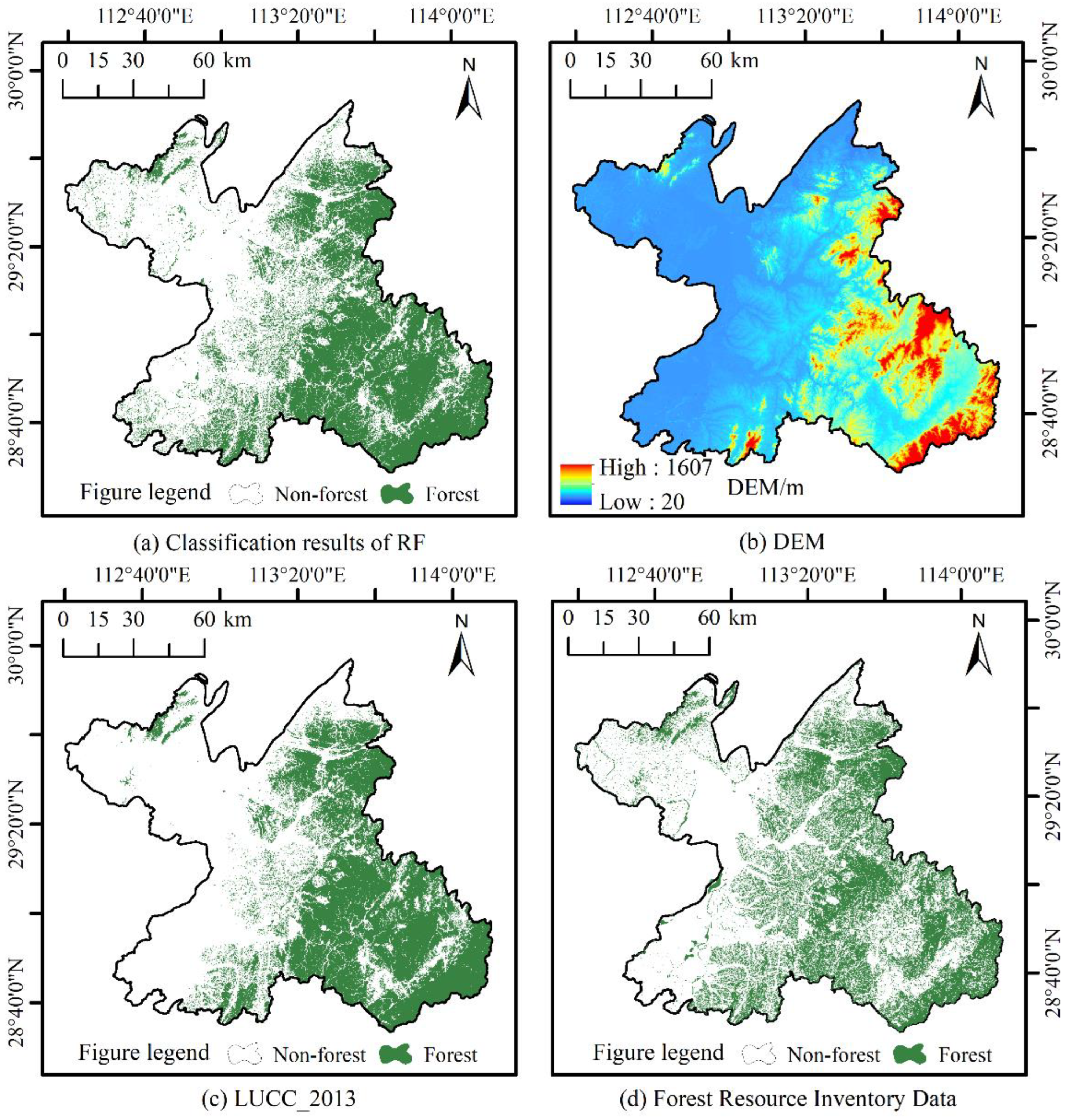
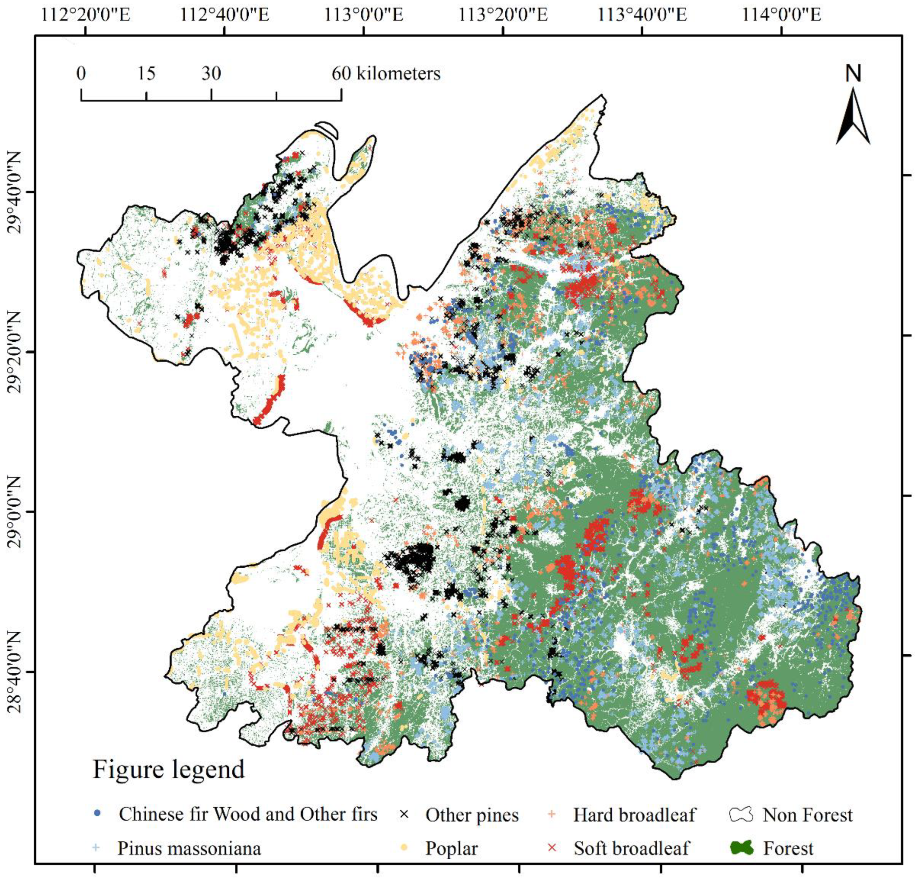
3.1. Classification Results for Dominant Species

In the present study, the forest cover of Yueyang City in 2013 was obtained by reclassifying the classification results, as shown in Figure 3. The results showed that the classification results of the RF algorithm and LUCC_2013 had a more extensive forest coverage and were closer to the spatial distribution characteristics of the Forest Resource Inventory data. The distribution range of some areas of LUCC_2013 was more obviously different from that of the Forest Resource Inventory data. In addition, the confusion matrix’s accuracy in the classification results of this study was evaluated using the forest/non-forest validation sample. As shown in

Table 3. Results of the forest/non-forest classification accuracy evaluation.

Category	UA (Pixels/%)	PA (Pixels/%)	OA (Pixels/%)	Kappa
Forest	92.86	86.67	93.79	0.9145
Water	96.88	96.87
Building lands	92.68	100
other lands	93.33	91.80

, the classification results of this study achieved an OA of 0.9379 and a Kappa coefficient of 0.9145. The forest area of the classification results of this study was 628,025 hm², while the forest area of LUCC_2013 was 579,738.6 hm². The forest area of Yueyang City in 2013 was about 634,200 hm² according to the forest coverage rate of 45.3%, which was the closest to the forest area of the classification result of this study (with a difference of 6175 hm²). Therefore, through visual interpretation, confusion matrix accuracy evaluation, and an area comparison analysis, this study’s forest/non-forest classification results had a high accuracy and can be used to refine the classification of dominant tree species in the secondary classification.

The dominant tree species in the forest range of the study area were classified using RF and SVM machine learning algorithms based on primary classification. The classification results of the two machine learning algorithms were compared with the reference distribution range of the Forest Resource Inventory data in the visual accuracy assessment (Figure 4). The comparison by visual interpretation showed that RF had the best classification results for the dominant tree species, with each category being closer to the reference distribution range. In the study area’s southeastern part, RF could better distinguish between Chinese fir wood and other firs, hard broadleaf species, and soft broadleaf species. In contrast, SVM had many misclassifications and classified other species as soft broadleaf. Similarly, RF and SVM produced misclassifications within the central and southern parts of the study area where there was mixed growth of individual tree species; this misclassification contributed to the inaccurate classification results, but RF still had the highest classification accuracy.

When comparing the validation samples with the classification results of the two classification algorithms, the results based on the accuracy calculations showed that the OA for classification using RF reached 0.8730 and the Kappa coefficient was 0.7747; the PA for both the poplar and soft broadleaf classes was higher than 0.9, and the classification was better. Still, the Chinese fir Wood and other firs and the other pines classes had a high error of omission; the misclassification of both classes was mainly for Pinus massoniana. In addition, the UA of the hard broadleaf category was only 0.6808, while it was above 0.7 for all other categories, with confusion occurring mainly between the poplar and soft broadleaf classes. The results of the accuracy evaluation are shown in

Table 4. Results of accuracy evaluation of dominant tree classification.

Method	Category	UA (Pixels/%)	PA (Pixels/%)	OA (Pixels/%)	Kappa
RF	Chinese fir wood and other firs	78.57	50.00	87.30	0.7747
	Pinus massoniana	70.69	85.42
	Other pines	72.09	62.00
	Poplar	97.62	97.62
	Hard broadleaf	68.08	68.09
	Soft broadleaf	92.84	95.92
SVM	Chinese fir wood and other firs	55.29	61.84	66.74	0.6006
	Pinus massoniana	63.37	75.29
	Other pines	70.33	68.09
	Poplar	92.31	100
	Hard broadleaf	57.53	65.63
	Soft broadleaf	60.38	35.56

.

Due to the complex topography of the Yueyang forest area, the classification units of the dominant tree species were fragmented, which resulted in a “salt and pepper noise” in the final classification results. The plural filtering method was required to remove, merge, and cluster the fragmented raster patches after classification using the RF algorithm to obtain smoother classification results while retaining the complete spatial structure after classification. The plural filter was a 3 × 3 window in which the 8 neighboring pixels of the current pixel were used as filters, which ensured that half of the 8 pixel values were the same before the corresponding pixel value could be changed. The results after plural filtering processes are shown in Figure 5.

3.2. Sample Data Filtering

The forest resource types were classified according to dominant trees, and the outliers were removed. The number of small groups after the screening was Chinese fir wood and other firs: 59,894; Pinus massoniana: 38,732; other pines: 21,865; poplar: 7170; hard broadleaf: 35,447; and soft broadleaf: 2581. In consideration of the fact that the sample data had to meet the modeling requirements, 1000 small class data from each dominant tree species category were randomly selected as modeling samples. The distribution of the modeling samples for each forest type is shown in Figure 6. The statistical results of the modeling sample points are shown in

Table 5. Results of accumulation statistics for the modeled sample sites in the study area.

Tree Species and Group	Number (Piece)	Min (m3·hm−2)	Max (m3·hm−2)	Average (m3·hm−2)	Standard Deviation (m3·hm−2)
Chinese fir wood and other firs	1000	6.04	99.11	34.21	22.75
Pinus massoniana	1000	6.92	61.67	31.48	13.72
Other pines	1000	6.00	85.11	40.40	21.86
Poplar	1000	12.22	93.33	47.75	15.59
Hard broadleaf	1000	8.97	70.41	37.25	17.29
Soft broadleaf	1000	3.97	87.14	32.32	19.83
Total	6000	3.97	99.11	-	-

.

3.3. Model Estimation Results and Accuracy Evaluation

The optimal forest carbon density model was selected as shown in

Table 6. Estimation accuracy of each dominant tree for different models.

Model	Tree Species and Group	R2	RMSE (t·hm−2)	MAE (t·hm−2)
MLR	Chinese fir wood and other firs	0.312	6.1289	4.9009
	Pinus massoniana	0.199	3.8054	3.1529
	Other pines	0.286	7.8201	6.4654
	Poplar	0.090	4.5832	3.9105
	Hard broadleaf	0.407	8.3541	6.8165
	Soft broadleaf	0.386	5.0962	4.0865
SVM	Chinese fir wood and other firs	0.342	6.6304	5.3309
	Pinus massoniana	0.249	5.3851	4.5164
	Other pines	0.294	7.7728	6.3876
	Poplar	0.165	4.3904	3.7138
	Hard broadleaf	0.445	8.0824	6.5731
	Soft broadleaf	0.431	4.8909	3.9716
RF	Chinese fir wood and other firs	0.5346	4.2854	3.6629
	Pinus massoniana	0.5363	2.2501	1.9841
	Other pines	0.6220	4.8738	4.1110
	Poplar	0.4054	3.1805	2.7538
	Hard broadleaf	0.7672	4.4380	3.7781
	Soft broadleaf	0.6534	2.9607	2.5848

. The remote sensing estimates of the forest carbon density model were calculated for 200 validation samples of each forest type; the model fitting effect is shown in Figure 7, and the results of the accuracy analysis and evaluation of the model showed that: the predicted mean forest carbon density for Chinese fir wood and other firs was 10.6051 t·hm⁻², the mean measured test pressure was 9.5397 t·hm⁻², the R² was 0.5346, the RMSE was 4.2854 t·hm⁻², and the MAE was 3.6629 t·hm⁻²; the predicted mean forest carbon density for Pinus massoniana was 9.4465 t·hm⁻², the mean measured test pressure was 9.1593 t·hm⁻², the R² was 0.5363, the RMSE was 2.2501 t·hm⁻², and the MAE was 1.9841 t·hm⁻²; the predicted mean forest carbon density for other pines was 17.4647 t·hm⁻², the mean measured test pressure was 17.6283 t·hm⁻², the R² was 0.6220, the RMSE was 4.8738 t·hm⁻², and the MAE was 4.1110 t·hm⁻²; the predicted mean forest carbon density for poplar was 15.8118 t·hm⁻², the mean measured test pressure was 15.0651 t·hm⁻², the R² was 0.4051, the RMSE was 3.1805 t·hm⁻², and the MAE was 2.7538 t·hm⁻²; the predicted mean forest carbon density for hard broadleaf was 22.1394 t·hm⁻², the mean measured test pressure was 21.7766 t·hm⁻², the R² was 0.7672, the RMSE was 4.4380 t·hm⁻², and the MAE was 3.7781 t·hm⁻²; and the predicted mean forest carbon density for soft broadleaf was 11.5278 t·hm⁻², the mean measured test pressure was 10.8526 t·hm⁻², the R² was 0.6534, the RMSE was 2.9607 t·hm⁻², and the MAE was 2.5848 t·hm⁻². This showed that the RF-based model predicted better results.

3.4. Forest Carbon Density Inversion Mapping

As shown in the spatial distribution map of the forest carbon density in Figure 8, the inversion results after classification according to the dominant tree species showed that the forest carbon stock in Yueyang City in 2013 was 10.2975 Tg, and the spatial distribution of forest carbon density values ranged from 3.06 to 62.80 t·hm⁻²; the inversion results without classification showed that the forest carbon stock was 10.7405 Tg, and the spatial distribution of forest carbon density values ranged from 4.64 to 31.96 t·hm⁻², showing that the carbon density values were severely overfitted. The estimation of the peak was excessively low. As shown in the b-plot in Figure 7, the largest area of the city’s forests with a carbon density between 10–20 t·hm⁻² reached 50.79% of the city’s forest area, followed by 20–30 t·hm⁻² and 3.06–10 t·hm⁻², which accounted for 26.25% and 17.52% of the city’s forest area, respectively; the area with a carbon density higher than 30 t·hm⁻² was the smallest and accounted for only 5.44%. Carbon stocks by stand type were dominated by other pines and soft broadleaf species, accounting for 40.37% of the city’s forest carbon stocks with 2.144 Tg and 2.0127 Tg, respectively; Chinese fir wood and other firs, Pinus massoniana, and hard broadleaf species had less with 1.5884 Tg, 1.7068 Tg, and 1.5795 Tg, respectively; while poplar had 1.2657 Tg of carbon stocks.

In terms of the geospatial distribution patterns (Figure 9), the forest carbon density in the city was higher in Huarong Xian (20.23 t·hm⁻²) and Xiangyin Xian (20.04 t·hm⁻²) and the lowest in Yueyang Xian (16.10 t·hm⁻²). The distribution pattern of the forest carbon stocks and carbon density of the arboreal forests in Yueyang City was slightly different, with Pingjiang Xian, which is located in the Mofu Mountain and Lianyun Mountain area and has a large forest cover. Many pine, fir, and broadleaf forest communities remain with carbon stocks reaching 5.1042 Tg. In contrast, the carbon stocks of other districts and counties were lower and ranged from 0.0579 to 1.6029 Tg, with Junshan Qu being the lowest.

4. Discussion

This study used the GEE platform to classify the forest extent of the study area into the dominant species. It then used machine learning algorithms to remotely classify the dominant species to estimate the forest carbon density in Yueyang in 2013. The training sample data for the model construction were randomly selected using the Forest Resource Inventory data for Yueyang City according to the division of the dominant trees. The final accuracy evaluation results showed that the prediction accuracy of the forest carbon density model was improved to a certain extent by using the non-linear model machine learning algorithm. Among the three models constructed (MLR, SVM, and RF), the RF model had the highest accuracy and had a certain applicability and feasibility. The estimation results according to the dominant trees were also significantly more reasonable than those without classification; thus, the estimation method in this study can be used as an important modeling method and approach in the field of large-scale remote sensing estimation of forest carbon density in the future. The spatial distribution of the forest carbon density estimated in this study ranged from 3.06 to 62.80 t·hm⁻² within the range of 0.00 to 67.35 t·hm⁻² previously calculated by scholars for forest carbon density in Hunan Province at a 500 m × 500 m resolution.

Given that different tree species had different root–trunk and canopy structures and different carbon sequestration capacities, it was necessary to differentiate between species to construct models for forest carbon density inversions [41]. Based on the optimal characteristics of different ground data sources, the stand types were divided according to the dominant species following the Guidelines for Monitoring Carbon Sinks in Afforestation Projects. The composite stand types (other pines, hard broadleaf, etc.) were calculated as the average of the species included in the study area to improve the carbon density estimation while making large-scale regional estimates. In this study, when using the RF method for feature-variable screening, ranking of the important features for the six forest types was dominated by the textural features of mean, variance, homogeneity, and entropy under the 9 × 9 window and bands 2, 3, 4, and 7 of the Landsat 8 OLI. In addition, since the slope, slope orientation, and elevation also affect the carbon sequestration capacity of forest trees, the inverse model of forest carbon density was constructed by combining the screened characteristic variables with three topographic factors to improve the model’s accuracy. However, the actual forest carbon density also was affected by various environmental factors and interference caused by various human factors, which affected the final prediction accuracy. In future related research, optical remote sensing and LiDAR data should be used to supplement the information at the vertical-structure level of forest stands to improve the accuracy of forest carbon stock estimation. This study focused on remote sensing estimation and the spatial distribution simulation of forest carbon stocks in the spatial dimension using machine learning algorithms; this can be followed by predicting forest growth time series in the temporal latitude. The division of forest carbon stocks into stand age groups for a more accurate estimation of forest carbon stocks is a worthy direction for future efforts to solve carbon sink problems using remote sensing.

5. Conclusions

This study was based on the GEE platform and used RF to delineate the dominant tree species in the forest range of the study area. In the forest/non-forest classification (primary classification), the OA reached 93.79% with a Kappa coefficient of 0.9145; in the dominant species classification (secondary classification), the OA reached 0.8730 with a Kappa coefficient of 0.7747. The results showed that using the GEE platform to classify the dominant tree species in large areas had better results and that the long-term monitoring of changes in the dominant tree species can be carried out on the GEE platform in the future using Landsat data, which also provide basic data on the distribution of tree species for forest carbon density estimation.

Based on Landsat 8 OLI remote sensing images, this study applied three different algorithms—MLR, SVM, and RF—to estimate the forest carbon density based on remote sensing factors such as spectral information, texture features, and terrain factors. The results showed that the traditional MLR model did not accurately represent the non-linear relationship between the predictor variables and the forest carbon density. At the same time, RF could better screen and combine the variables. Therefore, the R² (R² = 0.4054~0.7602) of the RF model was higher than both the MLR (R² = 0.0900~0.4070) and SVM (R² = 0.1650~0.4450), and the RMSE and MAE were significantly lower. Based on the distribution map of the remote sensing inversion results, it can be seen that the forest carbon stock in Yueyang City in 2013 was 10.2975 Tg, and the spatial distribution of forest carbon density ranged from 3.06 to 62.80 t·hm⁻². The distribution pattern of the city’s forest carbon stocks was dominated by Pingjiang Xian located in the Mofu Mountain and Lianyun Mountain area; its carbon stocks reached 5.1042 Tg. In addition, the average carbon density and carbon stocks of forests in all districts and counties of Yueyang City were inconsistent, which reflected the influence of different forest species, the forest cover area, and the forest quality on the carbon stocks.

References

1. Mikhaylov, A.; Moiseev, N.; Aleshin, K.; Burkhardt, T. Global climate change and greenhouse effect. Entrep. Sustain. Issues 2020, 7, 2897–2913. [Google Scholar] [CrossRef]
2. Liu, X.; Trogisch, S.; He, J.S.; Niklaus, P.A.; Bruelheide, H.; Tang, Z.; Erfmeier, A.; Scherer-Lorenzen, M.; Pietsch, K.A.; Yang, B.; et al. Tree species richness increases ecosystem carbon storage in subtropical forests. Proc. R. Soc. B 2018, 285, 20181240. [Google Scholar] [CrossRef] [PubMed] [Green Version]
3. Huang, L.; Zhou, M.; Lv, J.; Chen, K. Trends in global research in forest carbon sequestration: A bibliometric analysis. J. Clean. Prod. 2019, 252, 119908. [Google Scholar] [CrossRef]
4. Raihan, A.; Begum, R.A.; Said, M.N.M.; Pereira, J.J. Assessment of Carbon Stock in Forest Biomass and Emission Reduction Potential in Malaysia. Forests 2021, 12, 1294. [Google Scholar] [CrossRef]
5. Yin, S.; Gong, Z.; Gu, L.; Deng, Y.; Niu, Y. Driving forces of the efficiency of forest carbon sequestration production: Spatial panel data from the national forest inventory in China. J. Clean. Prod. 2021, 330, 129776. [Google Scholar] [CrossRef]
6. Felipe-Lucia, M.R.; Soliveres, S.; Penone, C.; Manning, P.; van der Plas, F.; Boch, S.; Prati, D.; Ammer, C.; Schall, P.; Gossner, M.M.; et al. Multiple forest attributes underpin the supply of multiple ecosystem services. Nat. Commun. 2018, 9, 4839. [Google Scholar] [CrossRef] [PubMed] [Green Version]
7. Ouyang, S.; Xiang, W.; Wang, X.; Xiao, W.; Chen, L.; Li, S.; Sun, H.; Deng, X.; Forrester, D.I.; Zeng, L.; et al. Effects of stand age, richness and density on productivity in subtropical forests in China. J. Ecol. 2019, 107, 2266–2277. [Google Scholar] [CrossRef]
8. Omer, G.; Mutanga, O.; Abdel-Rahman, E.M.; Adam, E. Performance of Support Vector Machines and Artificial Neural Network for Mapping Endangered Tree Species Using WorldView-2 Data in Dukuduku Forest, South Africa. IEEE J. Sel. Top. Appl. Earth Obs. Remote Sens. 2015, 8, 4825–4840. [Google Scholar] [CrossRef]
9. Meng, Y.; Cao, B.; Mao, P.; Dong, C.; Cao, X.; Qi, L.; Wang, M.; Wu, Y. Tree Species Distribution Change Study in Mount Tai Based on Landsat Remote Sensing Image Data. Forests 2020, 11, 130. [Google Scholar] [CrossRef] [Green Version]
10. Basheer, S.; Wang, X.; Farooque, A.A.; Nawaz, R.A.; Liu, K.; Adekanmbi, T.; Liu, S. Comparison of Land Use Land Cover Classifiers Using Different Satellite Imagery and Machine Learning Techniques. Remote Sens. 2022, 14, 4978. [Google Scholar] [CrossRef]
11. Poorazimy, M.; Shataee, S.; McRoberts, R.E.; Mohammadi, J. Integrating airborne laser scanning data, space-borne radar data and digital aerial imagery to estimate aboveground carbon stock in Hyrcanian forests, Iran. Remote Sens. Environ. 2020, 240, 111669. [Google Scholar] [CrossRef]
12. Gomes, L.C.; Faria, R.M.; de Souza, E.; Veloso, G.V.; Schaefer, C.E.G.; Fernandes Filho, E.I. Modelling and mapping soil organic carbon stocks in Brazil. Geoderma 2019, 340, 337–350. [Google Scholar] [CrossRef]
13. Khan, D.; Muneer, M.A.; Nisa, Z.U.; Shah, S.; Amir, M.; Saeed, S.; Uddin, S.; Munir, M.Z.; Gao, L.; Huang, H. Effect of climatic factors on stem biomass and carbon stock of Larix gmelinii and Betula platyphylla in Daxing’anling Mountain of Inner Mongolia, China. Adv. Meteorol. 2019, 10, 5692574. [Google Scholar] [CrossRef] [Green Version]
14. Pham, T.D.; Yokoya, N.; Bui, D.T.; Yoshino, K.; Friess, D.A. Remote Sensing Approaches for Monitoring Mangrove Species, Structure, and Biomass: Opportunities and Challenges. Remote Sens. 2019, 11, 230. [Google Scholar] [CrossRef] [Green Version]
15. Byrd, K.B.; Ballanti, L.; Thomas, N.; Nguyen, D.; Holmquist, J.R.; Simard, M.; Windham-Myers, L. A remote sensing-based model of tidal marsh aboveground carbon stocks for the conterminous United States. Isprs. J. Photogramm 2018, 139, 255–271. [Google Scholar] [CrossRef]
16. Su, Y.; Guo, Q.; Xue, B.; Hu, T.; Alvarez, O.; Tao, S.; Fang, J. Spatial distribution of forest aboveground biomass in China: Estimation through combination of spaceborne lidar, optical imagery, and forest inventory data. Remote Sens. Environ. 2016, 173, 187–199. [Google Scholar] [CrossRef] [Green Version]
17. Rodríguez-Veiga, P.; Wheeler, J.; Louis, V.; Tansey, K.; Balzter, H. Quantifying Forest Biomass Carbon Stocks From Space. Curr. For. Rep. 2017, 3, 1–18. [Google Scholar] [CrossRef] [Green Version]
18. Vicharnakorn, P.; Shrestha, R.P.; Nagai, M.; Salam, A.P.; Kiratiprayoon, S. Carbon Stock Assessment Using Remote Sensing and Forest Inventory Data in Savannakhet, Lao PDR. Remote Sens. 2014, 6, 5452–5479. [Google Scholar] [CrossRef] [Green Version]
19. Yan, E.; Lin, H.; Wang, G.; Sun, H. Improvement of Forest Carbon Estimation by Integration of Regression Modeling and Spectral Unmixing of Landsat Data. IEEE Geosci. Remote Sens. Lett. 2015, 12, 2003–2007. [Google Scholar] [CrossRef]
20. Zhang, J.; Lu, C.; Xu, H. Estimating aboveground biomass of Pinus densata-dominated forests using Landsat time series and permanent sample plot data. J. For. Res. 2019, 30, 1689–1706. [Google Scholar] [CrossRef]
21. Fassnacht, F.E.; Hartig, F.; Latifi, H.; Berger, C.; Hernández, J.; Corvalán, P.; Koch, B. Importance of sample size, data type and prediction method for remote sensing-based estimations of aboveground forest biomass. Remote Sens Environ. 2014, 154, 102–114. [Google Scholar] [CrossRef]
22. Lu, D.; Chen, Q.; Wang, G.; Liu, L.; Li, G.; Moran, E. A survey of remote sensing-based aboveground biomass estimation methods in forest ecosystems. Int. J. Digit. Earth 2014, 9, 63–105. [Google Scholar] [CrossRef]
23. Huang, W.; Li, W.; Xu, J.; Ma, X.; Li, C.; Liu, C. Hyperspectral Monitoring Driven by Machine Learning Methods for Grassland Above-Ground Biomass. Remote Sens. 2022, 14, 2086. [Google Scholar] [CrossRef]
24. Sekertekin, A.; Abdikan, S.; Marangoz, A.M. The acquisition of impervious surface area from LANDSAT 8 satellite sensor data using urban indices: A comparative analysis. Environ. Monit. Assess. 2018, 190, 381. [Google Scholar] [CrossRef] [PubMed]
25. Van der Werff, H.; Van der Meer, F. Sentinel-2A MSI and Landsat 8 OLI Provide Data Continuity for Geological Remote Sensing. Remote Sens. 2016, 8, 883. [Google Scholar] [CrossRef] [Green Version]
26. Mandanici, E.; Bitelli, G. Preliminary Comparison of Sentinel-2 and Landsat 8 Imagery for a Combined Use. Remote Sens. 2016, 8, 1014. [Google Scholar] [CrossRef] [Green Version]
27. Phiri, D.; Morgenroth, J.; Xu, C.; Hermosilla, T. Effects of pre-processing methods on Landsat OLI-8 land cover classification using OBIA and random forests classifier. Int. J. Appl. Earth Obs. Geoinf. ITC J. 2018, 73, 170–178. [Google Scholar] [CrossRef]
28. Ward, A.; Dargusch, P.; Thomas, S.; Liu, Y.; Fulton, E.A. A global estimate of carbon stored in the world’s mountain grasslands and shrublands, and the implications for climate policy. Glob. Environ. Chang. 2014, 28, 14–24. [Google Scholar] [CrossRef]
29. Yang, J.; Huang, X. The 30 m annual land cover dataset and its dynamics in China from 1990 to 2019. Earth Syst. Sci. Data 2021, 13, 3907–3925. [Google Scholar] [CrossRef]
30. Li, H.; Zhao, P.; Lei, Y.; Zeng, W. Comparison on Estimation of Wood Biomass Using Forest Inventory Data. Chin. For. Sci. Technol. 2012, 48, 44–52. [Google Scholar]
31. IPCC. IPCC Guidelines for National Greenhouse Gas Inventories: Agriculture, Forestry and Other Land Use; Institute of Global Environment Strategies: Tokyo, Japan, 2006.
32. The State Forestry Administration of the People’s Republic of China. Guidelines on Carbon Accounting and Monitoring for Afforestation Project; Standards Press of China: Beijing, China, 2014; pp. 30–33.
33. Randin, C.F.; Ashcroft, M.B.; Bolliger, J.; Cavender-Bares, J.; Coops, N.C.; Dullinger, S.; Dirnböck, T.; Eckert, S.; Ellis, E.; Fernández, N.; et al. Monitoring biodiversity in the Anthropocene using remote sensing in species distribution models. Remote Sens. Environ. 2020, 239, 111626. [Google Scholar] [CrossRef]
34. Zhao, Y.; Potgieter, A.B.; Zhang, M.; Wu, B.; Hammer, G.L. Predicting Wheat Yield at the Field Scale by Combining High-Resolution Sentinel-2 Satellite Imagery and Crop Modelling. Remote Sens. 2020, 12, 1024. [Google Scholar] [CrossRef] [Green Version]
35. Otgonbayar, M.; Atzberger, C.; Chambers, J.; Damdinsuren, A. Mapping pasture biomass in Mongolia using Partial Least Squares, Random Forest regression and Landsat 8 imagery. Int. J. Remote Sens. 2018, 40, 3204–3226. [Google Scholar] [CrossRef]
36. Li, C.; Li, Y.; Li, M. Improving Forest Aboveground Biomass (AGB) Estimation by Incorporating Crown Density and Using Landsat 8 OLI Images of a Subtropical Forest in Western Hunan in Central China. Forests 2019, 10, 104. [Google Scholar] [CrossRef] [Green Version]
37. Yang, B.; Zhang, Y.; Mao, X.; Lv, Y.; Shi, F.; Li, M. Mapping Spatiotemporal Changes in Forest Type and Aboveground Biomass from Landsat Long-Term Time-Series Analysis—A Case Study from Yaoluoping National Nature Reserve, Anhui Province of Eastern China. Remote Sens. 2022, 14, 2786. [Google Scholar] [CrossRef]
38. Lumbierres, M.; Méndez, P.F.; Bustamante, J.; Soriguer, R.; Santamaría, L. Modeling Biomass Production in Seasonal Wetlands Using MODIS NDVI Land Surface Phenology. Remote Sens. 2017, 9, 392. [Google Scholar] [CrossRef] [Green Version]
39. Coltri, P.P.; Zullo, J.; do Valle Goncalves, R.R.; Romani, L.A.S.; Pinto, H.S. Coffee crop’s biomass and carbon stock estimation with usage of high resolution satellites images. IEEE J.-STARS 2013, 6, 1786–1795. [Google Scholar]
40. Pandey, P.C.; Anand, A.; Srivastava, P.K. Spatial distribution of mangrove forest species and biomass assessment using field inventory and earth observation hyperspectral data. Biodivers Conserv. 2019, 28, 2143–2162. [Google Scholar] [CrossRef]
41. Gao, L.; Chai, G.; Zhang, X. Above-Ground Biomass Estimation of Plantation with Different Tree Species Using Airborne LiDAR and Hyperspectral Data. Remote Sens. 2022, 14, 2568. [Google Scholar] [CrossRef]
Figure 1. Geographical location and remote sensing image of Yueyang City.
Forests 13 02004 g001
Figure 2. Overview: graphical abstract of the research program. In Step 2, circles represent all samples. The red circle represents the removed abnormal samples, and the green circle represents the selected samples.
Forests 13 02004 g002
Figure 3. Forest/non-forest classification results. The (a) classification results of RF, (c) forest distribution map of LUCC_2013 and (d) forest distribution of Forest Resources Inventory data were compared and the accuracy was judged. Taking the elevation map of Yueyang City (b) as a reference, the distribution range of forest is compared.
Forests 13 02004 g003
Figure 4. Classification results of dominant trees based on different machine learning algorithms and the reference distribution range of Forest Resource Inventory data. The classification results of (a) RF, (b) SVM and (c) the dominant tree species distribution map of Forest Resource Inventory data were compared and the accuracy was judged.
Forests 13 02004 g004
Figure 5. A partial plot of the plural filtering of the RF classification results. (a) The initial classification results, (b) the results of the first plural filtering processes, (c) the result after two plural filtering processes, which had a better effect on the broken raster.
Forests 13 02004 g005
Figure 6. Distribution of modeling plots for each dominant tree in the study area. The dark blue circle represents Chinese fir wood and other firs, the light blue cross represents Pinus massoniana, the black oblique cross represents Other pines, the yellow circle represents Poplar, the yellow cross represents Hard broadleaf, and the red oblique cross represents Soft broadleaf.
Forests 13 02004 g006
Figure 7. Results of random forest model fitting for each dominant tree: (a) Chinese fir wood and other firs; (b) Pinus massoniana; (c) other pines; (d) poplar; (e) hard broadleaf; (f) soft broadleaf.
Forests 13 02004 g007
Figure 8. Spatial distribution of forest carbon density in Yueyang City based on random forest model (30 m × 30 m). (a) Unclassified random forest estimate with spatial distribution values ranging from 4.64 to 31.96 t·hm−2; (b) inversion results after classification according to the dominant tree species showing spatial distribution values ranging from 3.06 to 62.80 t·hm−2.
Forests 13 02004 g008
Figure 9. Spatial distribution patterns of average forest carbon density (a) and carbon stock (b) in Yueyang City based on RF estimates after delineating dominant tree species.
Forests 13 02004 g009