Abstract
The Asian longhorned beetle (ALB), Anoplophora glabripennis (Motschulsky), is one of the most harmful invasive alien species attacking hardwood trees. Increasing human activities have caused changes in the landscape patterns of ALB habitats, disrupting the habitat balance and weakening landscape-driven pest suppression. However, the relationship between landscape patterns (compositional and structural heterogeneity) and ALB populations has not been defined. In this study, we used remote sensing data to calculate landscape metrics and combined them with ground survey data. Using a multivariable linear regression model and a linear mixed model, we analyzed the relationship between landscape metrics and ALB populations and between forest stands attributes and ALB populations. The study results indicated that largest patch index (LPI), mean radius of gyration (GYRATE_MN), mean shape index (SHAPE_MN), and Shannon’s diversity index (SHDI) strongly influenced ALB populations at the landscape level. In addition, at the class level, only the forest class metrics LPI and aggregation index (AI) significantly impacted ALBs. The study also indicated that tree height (TH) and tree abundance (TREEAB) were good predictors of ALB populations.
1. Introduction
The Asian longhorned beetle (ALB), Anoplophora glabripennis (Motschulsky), is a polyphagous xylophage listed among the one hundred worst invasive alien species in the world and has caused devastating damage and economic loss to hardwood trees worldwide [1,2,3]. ALB is native to East Asia [4]. The earliest record of an ALB outbreak is from the Three-North Shelterbelts Forest Program in the 1970s, which used poplar, willow, and elm as the main tree species for afforestation efforts. Because of the lack of prior investigations, the tree species planted in the first phase of the Three Norths Protection Forest Program subsequently proved to be highly ALB-sensitive, leading to millions of trees’ death [2,5,6,7]. Economic losses caused by ALBs in China have been estimated to amount to 1.5 billion United States dollars per year [8,9].
ALB entered North America in the 1990s with solid wood packaging material from international trade [10]. The first area where ALB was discovered was New York, followed by several other American cities; in 2003, ALB also appeared in Canada [2,8,11]. One study showed that 35% of urban forests in the US are at risk of ALB infestation [12]. In 2001, ALB invasions were detected in Europe, first in Austria and then in many other countries, such as France and Germany [13]. Although ALB populations have not been found in natural forests in Europe and are currently only present in urban landscapes, this does not mean that ALB is not a risk in Europe [7].
Existing research suggests that various environmental factors influence the physiological activity of ALBs, the most significant of which is climate [5]. Temperature and effective cumulative temperature directly affect the developmental cycle of eggs, larvae, and adults, with differences in the number of generations, longevity, and fecundity of ALB reproduction under different temperature conditions [14,15,16,17,18]. Global warming also promotes the northward spread of ALBs’ suitable areas in China [19]. In addition, wind direction and speed affect the direction and distance of ALBs’ dispersal [20,21]. On the other hand, human social and economic activities also impact ALBs [22,23]. Increasing human activities have caused the loss and fragmentation of natural ecosystems, i.e., changes in land-use patterns [24]. The increase in land for agricultural production, the growth in land for construction, the continuous expansion of crop cultivation, and the removal of non-crop habitats have accelerated the degradation of forest ecosystems and the increasing homogeneity of landscape patterns [25]. The altered landscape pattern of ALBs habitats disrupts the balance of habitat ecosystems, reduces biodiversity within habitats, affects the ecological control function of natural enemies, and weakens landscape-driven pest suppression [26,27]. These lay the groundwork for the outbreak of ALBs within a landscape.
With the increasing advances in remote sensing technology, remote sensing images have better resolution and have become more useful for studying landscape patterns [28,29,30]. Ecologists have widely discussed the impact of landscape patterns on insects [31]. Central to the study of landscape patterns is heterogeneity, and it was determined by two aspects: (i) landscape composition (diversity of landscape features and habitat types) and (ii) landscape configuration (number, size, and connectivity of habitat patches) [32,33,34]. In landscape pattern research, landscape metrics are often required to assess patch structure changes within ecosystems and diagnose structural and functional relationships between different classes and patches within classes [35,36]. Over time, changes in landscape metrics can serve as solid support for quantifying ecological processes within a landscape [37,38].
Many studies emphasized the impact of landscape configuration (compositional and structural heterogeneity) on certain types of insects. For example, butterfly species diversity can be positively influenced by heterogeneity in landscape composition and negatively impacted by land-use intensity [39]. Landscape heterogeneity positively affects wasp and bee species richness [40], and different bee populations respond differently to landscape heterogeneity [41], meanwhile landscape heterogeneity is positively correlated with the functional diversity of bees [42]. In semi-natural habitats, the species richness and community composition of hoverflies are also determined by landscape heterogeneity [43]. Scholars also used landscape patterns to discuss the interactions between ecosystems and organisms to build more complex correlation models. The interaction of these abiotic and biotic landscape features (including tree species phenotypes, soil properties, forest stand attributes, topographic characteristics, climatic conditions, etc.) has an impact on organisms, forming a complex spatio-temporal dynamic mosaic [31,44,45]. For example, Wang [46] studied the mixed effects of forest stand attributes and landscape patterns on arthropod communities within a natural poplar forest in Xinjiang, China, and discussed the optimal scale of the response of arthropods to environmental factors within the forest.
The occurrence of pests is usually related to landscape patterns [31,44]. However, landscape research on ALBs remains scarce. Understanding the response of ALB populations to landscape pattern characteristics and forest stand attributes in nature can help devise better ALB ecological control strategies. Our study mainly focuses on three aspects: (1) the influence of landscape patterns on the population of ALBs; (2) the influence of forest site conditions on ALBs; and (3) the discussion of the two aspects above to provide suggestions for forest pest management.
2. Materials and Methods
2.1. Study Regions
The study was conducted in Jiuquan (38°09′~42°48′ N; 92°20′~100°20′ E), in northwestern Gansu Province, China. The climate is semi-desert arid, with an average annual rainfall of 84 mm and average yearly evaporation of 2141.4 mm—27.3 times the rainfall. We selected 11 independent circular landscapes (radius = 500 m) based on remote sensing images; each quarter of the landscape contained one sampling site. The distance between each landscape was more than 5 km to avoid spatial overlaps. We surveyed the broad-leaved trees spread in sampling sites.; the sampling site size was 20 × 30 m2, resulting in 44 sampling sites (Figure 1).
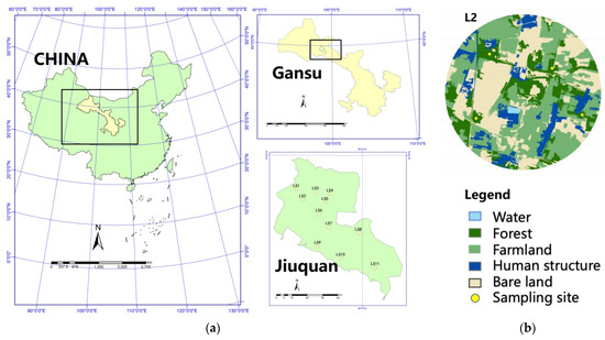
Figure 1.
Study area in northwestern Gansu, China. (a) Eleven circular landscapes with a 500 m radius in Jiuquan. (b) Example locations of four sampling sites in landscape2 (L2).
2.2. Surveys
We conducted extensive visual surveys of ALB damage in each landscape with vehicles and on foot from July to August 2019 [47]. In each landscape, we identified the current and recent outbreaks of ALBs as sampling sites according to new emergence holes, fallen leaves and branches, new frass holes, and traces of adult ALBs. We recorded the total number of trees and tree species in sampling sites, randomly chose ten trees within, counted emergence holes and new frass holes in them, and added up their number to calculate the average number of holes per tree as the indicator of the population of ALBs (y) (Figure A1). The tree height (TH), diameter at breast height (DBH), tree crown width (TCW), and the leaf loss rate of selected trees were measured. In addition, all damaged trees were counted to obtain the damage rate in each sample site. Finally, we grouped the data into two categories based on the usage type of the sampling sites (1. farmland shelterbelt, 2. street trees) and measured the distance from all sampling sites to the Beida River (a river across Jiuquan).
2.3. Landscape Metrics and Mapping
Gaofen-1 satellite images were used as source data to build the land-use map. We chose cloud-free images from July–August 2018 (broad-leaved trees are relatively easy to identify in summer). Next, we preprocessed the original Gaofen-1 images in ENVI (Version 5.3, Boulder, CO, USA) to eliminate errors, improve image quality, and perform image fusion and mosaic. Finally, we made a new image with a 2-m resolution to construct the land-use map. Based on ground surveys, we classified the image into five land cover species: water, forest, farmland, human structures (including roads), and bare land (including unused land). The image classification was obtained with eCognition (Veision 8.9, Westminster, CO, USA) using the following parameters: multiresolution segmentation scale parameter, 200; shape, 0.1; compactness, 0.5; water area classification, NDWI ≥ 0.3. The parameters were tested by several rounds of classifications, giving the most appropriate results. Finally, ArcGIS (Version 10.1, Redlands, CO, USA) was used to convert the land-use classification map format.
Landscape metrics were calculated in Fragstats (Version 4.2.1, Amherst, MA, USA) [36]. A total of twenty-two landscape level metrics and seventeen class level metrics were calculated and used as preliminary data to get the correlation matrix separately.
2.4. Data Analysis
All statistical analyses were performed in R (Version 4.0.2, Vienna, Austria) [48]. We used the MASS package [49] to conduct variable selection using a stepwise algorithm, the car package [50] to calculate multicollinearity, the lmerTest package [51] to use the Linear Mixed Model, and the ggplot2 package [52] for plotting.
The main calculation included three sections: (1) the correlation between landscape-level metrics and the population of ALBs; (2) the correlation between class-level metrics and the population of ALBs; (3) the correlation between forest stands attributes and the population of ALBs.
To normalize the population data of ALBs, we performed a logarithmic transformation (log(y + 1)) of the population of ALBs (y), and get (ly) to represent the population of ALBs [43,46,53].
The landscape metrics were filtered according to their correlation (Figure 2). Metrics strongly correlated with other landscape metrics (r > |0.7|) were removed. Only independent and representative landscape metrics were retained. Many metrics are wholly or partially redundant and quantify similar or identical aspects of the landscape pattern. In most cases, the redundant metrics will be highly or even perfectly correlated [54].
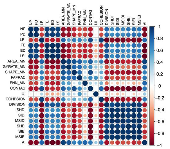
Figure 2.
Correlation matrix for landscape metrics, using the landscape level as an example.
The calculation in Section 1 and Section 2 were analyzed using a multivariable linear regression model, and a stepwise regression method was used to filter the variables. We tested the result using quantile-quantile plots and multicollinearity using a Variance Inflation Factor (VIF) [50].
To eliminate the effects of different sampling site types and distance to the Beida River on ALBs, in Calculation Section 3, we used Linear Mixed Model (LMM). All the forest stand attributes were as follows: I. tree height (TH); II. diameter at breast height (DBH); III. tree crown width (TCW); IV. tree abundance (TREEAB); V. tree species diversity (TSD); VI. sample site types (TYPE), 1: farmland shelterbelt, 2: street trees; and VII. distance to the Beida River (DIST), 1. <10 km 2. >10 km. VI and VII are random factors. The Akaike information criterion (AIC) was used to evaluate the models.
3. Results
The total number of trees surveyed in the 11 landscapes was 1892, of which 366 trees were infested with ALBs, with a damage rate of 19.3%. A total of 3568 holes (emergence holes and frass holes) were recorded in this study. Within all landscapes, bare land was the dominant land cover type (Figure 3) and had the most extensive area.
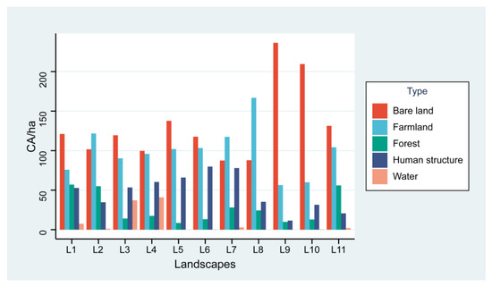
Figure 3.
Area of each land cover in hectares. CA (total class area, ha), L1-L11 (landscape 1–landscape 11).
3.1. Correlation of Landscape-Level Metrics and ALBs
In this part, eight landscape metrics were involved in the analysis: NP, LPI, GYRATE_MN, SHAPE_MN, PAFRAC, ENN_MN, IJI, and SHDI. After stepwise regression, non-significant variables were deleted to refit the model. The remaining four variables were LPI (largest patch index), GYRATE_MN (mean radius of gyration), SHAPE_MN (mean shape index), and SHDI (Shannon’s diversity index), model R2 = 0.7873, p = 0.0324 * (Table 1).

Table 1.
The significance of the landscape metrics involved in the multiple regression and the degree of model fit (significance: * p < 0.05, ** p < 0.01).
The effect of LPI on ALBs was most significant (E = −1.6686, p = 0.0087 **), and the impact of GYRATE_MN on ALBs was highly significantly positive (E = 1.2231, p = 0.0087 *). The impact of SHAPE_MN on ALBs was highly significantly negative (E =−1.96866, p = 0.0153 *), and SHDI had a highly significant negative correlation on ALBs (E = −2.1956, p = 0.0187 *) (Table 1).
3.2. Correlation of Class-Level Metrics and ALBs
All land cover metrics were analyzed separately. Only forest class metrics were statistically significant. LPI, LSI, AREA_MN, GYRATE_MN, SHAPE_MN, ENN_MN, IJI, and AI were selected to participate in the multiple regression fitting. After stepwise regression, the insignificant variables were removed and fitted again, resulting in the remaining two variables, LPI and AI (aggregation index); p = 0.02615 *, Adj-R2 = 0.4973 (Table 1).
LPI had a significant positive correlation with ALBs (E = −0.5809, p = 0.0206 *), and AI had a significant negative correlation with ALBs (E = 0.652, p = 0.0121 *).
3.3. Correlation of Forests Stand Attributes and ALBs
The results of the LMM showed that TH and TREEAB in forest stand attributes were significantly correlated with the population of ALBs. TH was significantly positively correlated with the population of ALBs, and TREEAB was highly significantly negatively correlated with the population of ALBs. Among all models, Model 6 had the smallest AIC value and fitted the best (Table 2).
Table 2.
The variables used in LMM models, their significance, and the ranking of all models using the Akaike information criterion (AIC) values (from largest to smallest). I. Tree height (TH); II. diameter at breast height (DBH); III. tree crown width (TCW); IV. tree abundance (TREEAB); V. tree species diversity (TSD); VI. sample site types (1|TYPE), 1: farmland shelterbelt, 2: street trees; and VII. distance to the Beida River (1|DIST), 1: <10 km 2: >10 km (significance: * p < 0.05, ** p < 0.01).
LMMs also showed that two random factors influenced the model fitness. The fitted regression lines of ly with TH and TREEAB have different slopes within different DIST and TYPE (Figure 4). Still, neither random factor passed the significance test (all random factors’ p-values > 0.05).
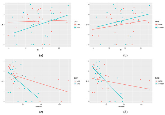
Figure 4.
ALBs’ population data were categorized according to sampling sites and fitted with TH and TREEAB separately; (a,c) showed the influence of the distance to the Beida River, (b,d) showed the influence of the forest type.
4. Discussion
4.1. Landscape-Level Matrices and ALBs
Among the landscape-level metrics, those that impact the population of ALBs are mainly focused on the percentage of the landscape covered by the largest patch in the landscape, patch shape, patch continuity, and patch richness.
The value of largest patch index (LPI) showed a highly significant negative correlation with the population of ALBs, mainly because the bare ground was the largest landscape type in this study in terms of area and number of patches (Figure 3). Such conditions result in reduced resources available to adult ALBs within the landscape, requiring migration to survive and reproduce. Adult ALBs are weak in flight [55], and need stepping stones to be able to fly farther. When the bare ground was the dominant patch type in the landscape, the lack of vegetation, trees, shade, and habitat increased the cost of finding new habitats for ALBs, increased mortality, and limited populations due to habitat size [56,57].
The mean radius of gyration (GYRATE_MN) was significantly positively correlated with the population of ALBs, and Shannon’s diversity index (SHDI) was significantly negatively correlated with the population of ALBs. One of these metrics represents the continuity of landscape patches, and the other represents the richness and evenness of landscape patches. Both metrics reflect the degree of fragmentation of the landscape. Ecologists have widely demonstrated the fragmentation of patches and reduced landscape connectivity to be a significant cause of biodiversity loss [40,58,59]. GYRATE_MN is an index that reflects landscape continuity and can be described as the average distance an organism moves from a random starting point in a patch in a random direction without leaving the patch. Ecologically, the extent of a patch is considered more important relative to the area of the patch [36]. The extent of the patch is usually associated with continuity as a measure of the extensiveness of the habitat, and continuity is a vital element of landscape structure [36,60]. ALBs would have more opportunities to fly and disperse in patches with good continuity to find suitable hosts to complete the life cycle. Patches function as stepping stones for ALBs, allowing them to fly longer distances. Moreover, the greater the patch extension, the greater the probability that it would be adjacent to other patches in the landscape, thus increasing dispersal success.
The SHDI index represents landscape heterogeneity [40]. Patch fragmentation strongly influences landscape heterogeneity, increasing patch spacing, reducing patch size, and decreasing available resources. This strongly affects population dynamics in the landscape and increases the risk of extinction [61]. A study by Slattery [62] found that agricultural expansion areas caused forest landscapes to become fragmented, with patches less aggregated, more complex in shape, and with longer edges negatively affecting the meiofauna that settled in the forest. The same situation occurred in our study area. With increased fragmentation and expansion of farming, the number of trees in the landscape became smaller and small patches of forests were randomly distributed and unconnected. Longer habitat distances would make it more difficult for ALBs to spread. Therefore, the fragmentation of patches and the reduction in connectivity brought about by abundant land use can directly affect the population size of ALBs. However, this effect is not specific to ALBs; it also negatively impacts other forest-dwelling organisms.
In terms of landscape shape, mean shape index (SHAPE_MN) negatively correlated with the number of ALBs. This index relates to the complexity of the shape of patches within the landscape. The higher the value, the more complex the patches’ shape. It is generally accepted in ecology that the shape of landscape patches significantly impacts the migration of animals, plants, and materials to and from the landscape. Stamps [63] concluded that patch shape affects animal migration when a boundary’s contrast is low (i.e., the landscape is traversable). Colling et al. [64] similarly found this issue in their study of ground-dwelling beetles, where landscape shape significantly influenced the behavior of ground-dwelling beetles crossing patches when the landscape boundary was traversable. In a study of the effects of urban green space landscapes on insect densities in Beijing, Su [65] found that the degree of irregularity in the shape of green space patches led to an increase in habitat edge effects, which, in turn, exacerbated species disturbance in the habitat and negatively affected insect densities. In our study, because of the flight capabilities of ALBs, we considered the landscapes in our research to be traversable. Our conclusion was consistent with Su’s that landscapes with high SHAPE_MN had lower populations of ALBs. We speculated that a complex landscape shape exposes ALBs to more disturbances, such as pesticide use, predator predation (elevated predator abundance and predation rates in border areas), or loss of habitat due to the severe damage that would cause nearby villagers to cut down trees [66].
4.2. Forest Patch Metrics and ALBs
The largest patch percentage of forest patches at the class level inhibits the population of ALBs, which may be due to the following reasons: 1. a large homogeneous forest patch has more trees and species in its ecosystem. Such an ecosystem is more stable and has better biodiversity and forest pest resistance than a small, fragmented forest patch. 2. The tree species in our study’s large homogeneous forest patches were dominated by Populus alba var. pyramidalis. In contrast, the other small, fragmented forest patches were sheltered forests planted in the 1970s during the implementation of the Three-North Shelterbelts Forest Program, with Populus gansuensis left around the farmland after decades of damage by ALBs. Plenty of research demonstrated that Populus alba var. pyramidalis was highly resistant to ALBs [6].
The degree of patch aggregation was significantly and positively correlated with the population of ALBs, consistent with our findings at the landscape level that the degree of aggregation of fragmented forest patches can dramatically affect the dispersal of adult ALBs in the landscape. The closer the non-adjacent forest patches were to each other, the easier it was for adult ALBs to complete their life cycle by flying to new hosts.
4.3. Forest Stand Attributes and ALBs
We discussed the effects of the two random factors for forest stand attributes and ALBs separately. Firstly, in both the tree height (TH) and tree abundance (TREEAB) linear regression models (Figure 4b,d), the slope is higher for models >10 km. This may be because of the arid climatic conditions, and trees grew poorly in areas far from the water source. However, the reasons for this may be more complex than we expect, considering a range of biotic and abiotic factors such as soil, climate, and topography. Moreover, there was no difference in linear regression models of the TH between farmland shelterbelt and street trees. However, the slopes differed significantly in TREEAB. We suggest that the random factors impact the population of ALBs, and due to the multiple factors, the precise reason for this phenomenon remains a gap. We will continue our research about these random factors.
For tree height, few were found in the literature on the relationship between tree height and pest population size. In our study, we found tree height to be a vital predictor of the population of ALBs, and this phenomenon was more pronounced in landscapes further away from the water area (Figure 4a). Wang [67] described the relationship between biomass and tree height, and believes that small-scale accurate tree height data should be used instead of large-scale average height data when predicting forest biomass. Small-scale precise tree heights were positively correlated with forest biomass. Hui et al. [68] also found a significant correlation between tree height and biomass level in their study of the relationship between forest biomass and tree productivity. Our conclusions would make this point even more well-founded.
In terms of tree abundance, it had a suppressive effect on the population of ALBs. Combined with the field survey, we believe that this result was consistent with the results in Section 3.2. The higher the total number of trees, the more stable its ecosystem. We suggest that landscape and ecology research about invasive pests such as ALB should consider forest stand attributes.
5. Conclusions
We used remote sensing and field survey data along with stepwise regression models and LMM models to calculate the relationship between landscape patterns and the population of Asian longhorned beetles. This is the first study on the ecological relationship between landscape patterns and ALBs. At the same time, our research also supplements the landscape pattern research of forest borer pests. Such research is currently very scarce. We found that overall landscape patch connectivity, fragmentation, edge complexity, and the degree of aggregation and size of forest patches all significantly affected ALBs. The results represent the forest patch level and the landscape level from small-scale to large-scale. Our conclusions serve as a suitable warning for modern societies, where natural ecosystems are increasingly fragmented and diminished; policymakers should control agricultural sprawl to protect biodiversity. Our findings also explain the regularity of the population of ALBs from the landscape ecology perspective, reveal the characteristics of forests in susceptible regions, and provide essential knowledge for the prevention and early detection of ALBs.
Author Contributions
Conceptualization, C.Y., S.Z. and L.R.; formal analysis, C.Y. and Z.Z.; funding acquisition, S.Z. and L.R.; investigation, C.Y.; methodology, C.Y.; resources, S.Z.; software, C.Y. and Z.Z.; supervision, S.Z.; visualization, C.Y. and L.R.; writing—original draft, C.Y.; writing—review and editing, S.Z. and L.R. All authors have read and agreed to the published version of the manuscript.
Funding
This research was supported by the National Key R & D Program of China (2022YFD1401000); National Key R & D Program of China (2022YFD1400400).
Data Availability Statement
Not applicable.
Acknowledgments
We appreciate the help of Siwei Guo and Quan Zhou from Beijing Forestry University for the field survey, and Xingwu Zhou from Forestry and Grassland Administration of Suzhou District, Jiuquan for the gentle help in geographic data support.
Conflicts of Interest
The authors declare no conflict of interest.
Appendix A

Figure A1.
The population data of ALBs in each landscape from L1-L11(landscape 1–landscape 11). y (the average number of emergence holes and frass holes in each landscape).
Figure A1.
The population data of ALBs in each landscape from L1-L11(landscape 1–landscape 11). y (the average number of emergence holes and frass holes in each landscape).

References
- Lowe, S.; Browne, M.; Boudjelas, S.; De Poorter, M. 100 of the World’s Worst Invasive Alien Species: A Selection from the Global Invasive Species Database; Invasive Species Specialist Group: Auckland, New Zealand, 2000; Volume 12. [Google Scholar]
- Haack, R.A.; Herard, F.; Sun, J.; Turgeon, J.J. Managing invasive populations of Asian longhorned beetle and citrus longhorned beetle: A worldwide perspective. Annu. Rev. Entomol. 2010, 55, 521–546. [Google Scholar] [CrossRef]
- Meng, P.S.; Hoover, K.; Keena, M.A. Asian Longhorned Beetle (Coleoptera: Cerambycidae), an Introduced Pest of Maple and Other Hardwood Trees in North America and Europe. J. Integr. Pest Manag. 2015, 6, 1–13. [Google Scholar] [CrossRef]
- Lingafelter, S.W.; Hoebeke, E.R. Revision of the Genus Anoplophora (Coleoptera: Cerambycidae); Entomological Society of Washington: Washington, DC, USA, 2002; ISBN 0-9720714-1-5. [Google Scholar]
- Wang, Z. Study on the Occurrence Dynamics of Anoplophora glabripennis (Coleoptera: Cerambycidae) and Its Control Measures. PhD Thesis, Northeast Forestry University, Harbin, China, 2004. [Google Scholar]
- Luo, Y.; Liu, R.; Xu, Z. Theories and technologies of ecologically regulating poplar longhorned beetle disaster in shelter forest. J. Beijing For. Univ. 2002, 24, 160–164. [Google Scholar]
- Javal, M.; Roques, A.; Haran, J.; Hérard, F.; Keena, M.; Roux, G. Complex invasion history of the Asian long-horned beetle: Fifteen years after first detection in Europe. J. Pest Sci. 2017, 92, 173–187. [Google Scholar] [CrossRef]
- Hu, J.; Angeli, S.; Schuetz, S.; Luo, Y.; Hajek, A.E. Ecology and management of exotic and endemic Asian longhorned beetle Anoplophora glabripennis. Agric. For. Entomol. 2009, 11, 359–375. [Google Scholar] [CrossRef]
- Golec, J.R.; Li, F.; Cao, L.M.; Wang, X.Y.; Duan, J.J. Mortality factors of Anoplophora glabripennis (Coleoptera: Cerambycidae) infesting Salix and Populus in central, northwest, and northeast China. Biol. Control 2018, 126, 198–208. [Google Scholar] [CrossRef]
- Haack, R.A. Exotic bark-and wood-boring Coleoptera in the United States: Recent establishments and interceptions. Can. J. For. Res. 2006, 36, 269–288. [Google Scholar] [CrossRef]
- Bartell, S.M.; Nair, S.K. Establishment risks for invasive species. Risk Anal. 2004, 24, 833–845. [Google Scholar] [CrossRef] [PubMed]
- Nowak, D.J.; Pasek, J.E.; Sequeira, R.A.; Crane, D.E.; Mastro, V.C. Potential effect of Anoplophora glabripennis (Coleoptera: Cerambycidae) on urban trees in the United States. J. Econ. Entomol. 2001, 94, 116–122. [Google Scholar] [CrossRef] [PubMed]
- Hérard, F.; Ciampitti, M.; Maspero, M.; Krehan, H.; Benker, U.; Boegel, C.; Schrage, R.; Bouhot-Delduc, L.; Bialooki, P. Anoplophora species in Europe: Infestations and management processes 1. EPPO Bull. 2006, 36, 470–474. [Google Scholar] [CrossRef]
- Hua, L.; Li, S.; Zhang, X. Coleoptera, Cerambycidae. In Iconography of Forest Insects Hunan China; Peng, J., Liu, W., Eds.; Hunan Scientific and Technical Publishing House: Changsha, China, 1992; pp. 467–524. [Google Scholar]
- Yang, Z.; Wang, X.; Yao, W.; Chu, X.; Li, P. Generation differentiation and effective accumulated temperature of Anoplophora glabripennis (Motsch.). For. Pest Dis. 2000, 19, 12–14. [Google Scholar]
- Keena, M.A. Effects of temperature on Anoplophora glabripennis (Coleoptera: Cerambycidae) adult survival, reproduction, and egg hatch. Environ. Entomol. 2006, 35, 912–921. [Google Scholar] [CrossRef]
- Keena, M.A.; Moore, P.M. Effects of temperature on Anoplophora glabripennis (Coleoptera: Cerambycidae) larvae and pupae. Env. Entomol 2010, 39, 1323–1335. [Google Scholar] [CrossRef] [PubMed]
- Sanchez, V.; Keena, M.A. Development of the teneral adult Anoplophora glabripennis (Coleoptera: Cerambycidae): Time to initiate and completely bore out of maple wood. Env. Entomol 2013, 42, 1–6. [Google Scholar] [CrossRef]
- Wang, P.; Du, W.; Li, M. Global warming and adaptive changes of forest pests. J. Northwest For. Univ. 2011, 26, 124–128. [Google Scholar]
- Smith, M.T.; Tobin, P.C.; Bancroft, J.; Li, G.H.; Gao, R.T. Dispersal and spatiotemporal dynamics of Asian longhorned beetle (Coleoptera: Cerambycidae) in China. Environ. Entomol. 2004, 33, 435–442. [Google Scholar] [CrossRef]
- Williams, D.W.; Li, G.; Gao, R. Tracking movements of individual Anoplophora glabripennis (Coleoptera: Cerambycidae) adults: Application of harmonic radar. Environ. Entomol. 2004, 33, 644–649. [Google Scholar] [CrossRef]
- Colunga-Garcia, M.; Haack, R.A.; Magarey, R.A.; Margosian, M.L. Modeling spatial establishment patterns of exotic forest insects in urban areas in relation to tree cover and propagule pressure. J. Econ. Entomol. 2010, 103, 108–118. [Google Scholar] [CrossRef]
- Huang, J.; Lu, X.; Liu, H.; Zong, S. The Driving Forces of Anoplophora glabripennis Have Spatial Spillover Effects. Forests 2021, 12, 1678. [Google Scholar] [CrossRef]
- Brockerhoff, E.G.; Jactel, H.; Parrotta, J.A.; Ferraz, S.F. Role of eucalypt and other planted forests in biodiversity conservation and the provision of biodiversity-related ecosystem services. For. Ecol. Manag. 2013, 301, 43–50. [Google Scholar] [CrossRef]
- Lu, Z.; Ouyang, F.; Zhang, Y.; Guan, X.; Men, X. Impacts of landscape patterns on populations of the wheat mites, Petrobia latens (Müller) and Penthaleus major (Duges), in the North China Plain. Acta Ecol. Sin. 2016, 36, 4447–4455. [Google Scholar] [CrossRef]
- Bianchi, F.J.J.A.; Booij, C.J.H.; Tscharntke, T. Sustainable pest regulation in agricultural landscapes: A review on landscape composition, biodiversity and natural pest control. Proc. R. Soc. B Biol. Sci. 2006, 273, 1715–1727. [Google Scholar] [CrossRef] [PubMed]
- Ouyang, F.; Ge, F. Effects of agricultural landscape patterns on insects. Chin. J. Appl. Entomol. 2011, 48, 1177–1183. [Google Scholar]
- Kowe, P.; Mutanga, O.; Dube, T. Advancements in the remote sensing of landscape pattern of urban green spaces and vegetation fragmentation. Int. J. Remote Sens. 2021, 42, 3797–3832. [Google Scholar] [CrossRef]
- Rodman, K.C.; Andrus, R.A.; Butkiewicz, C.L.; Chapman, T.B.; Gill, N.S.; Harvey, B.J.; Kulakowski, D.; Tutland, N.J.; Veblen, T.T.; Hart, S.J. Effects of Bark Beetle Outbreaks on Forest Landscape Pattern in the Southern Rocky Mountains, USA. Remote Sens. 2021, 13, 1089. [Google Scholar] [CrossRef]
- Pazúr, R.; Price, B.; Atkinson, P.M. Fine temporal resolution satellite sensors with global coverage: An opportunity for landscape ecologists. Landsc. Ecol. 2021, 36, 2199–2213. [Google Scholar] [CrossRef]
- Ferrenberg, S. Landscape Features and Processes Influencing Forest Pest Dynamics. Curr. Landsc. Ecol. Rep. 2016, 1, 19–29. [Google Scholar] [CrossRef][Green Version]
- Dominik, C.; Seppelt, R.; Horgan, F.G.; Settele, J.; Vaclavik, T. Landscape composition, configuration, and trophic interactions shape arthropod communities in rice agroecosystems. J. Appl. Ecol. 2018, 55, 2461–2472. [Google Scholar] [CrossRef]
- Seppelt, R.; Beckmann, M.; Ceausu, S.; Cord, A.F.; Gerstner, K.; Gurevitch, J.; Kambach, S.; Klotz, S.; Mendenhall, C.; Phillips, H.R.P.; et al. Harmonizing Biodiversity Conservation and Productivity in the Context of Increasing Demands on Landscapes. Bioscience 2016, 66, 890–896. [Google Scholar] [CrossRef]
- Fahrig, L.; Baudry, J.; Brotons, L.; Burel, F.G.; Crist, T.O.; Fuller, R.J.; Sirami, C.; Siriwardena, G.M.; Martin, J.L. Functional landscape heterogeneity and animal biodiversity in agricultural landscapes. Ecol Lett 2011, 14, 101–112. [Google Scholar] [CrossRef]
- McGarigal, K.; Cushman, S.A.; Neel, M.C.; Ene, E. FRAGSTATS: Spatial Pattern Analysis Program for Categorical and Continuous Maps. Available online: http://www.umass.edu/landeco/research/fragstats/fragstats.html (accessed on 10 May 2020).
- McGarigal, K. FRAGSTATS Help. Available online: http://www.umass.edu/landeco/research/fragstats/documents/fragstats.help.4.2.pdf (accessed on 21 April 2020).
- Syrbe, R.-U.; Walz, U. Spatial indicators for the assessment of ecosystem services: Providing, benefiting and connecting areas and landscape metrics. Ecol. Indic. 2012, 21, 80–88. [Google Scholar] [CrossRef]
- Badora, K.; Wróbel, R. Changes in the Spatial Structure of the Landscape of Isolated Forest Complexes in the 19th and 20th Centuries and Their Potential Effects on Supporting Ecosystem Services Related to the Protection of Biodiversity Using the Example of the Niemodlin Forests (SW Poland). Sustainability 2020, 12, 4237. [Google Scholar] [CrossRef]
- Perović, D.; Gámez-Virués, S.; Börschig, C.; Klein, A.-M.; Krauss, J.; Steckel, J.; Rothenwöhrer, C.; Erasmi, S.; Tscharntke, T.; Westphal, C.; et al. Configurational landscape heterogeneity shapes functional community composition of grassland butterflies. J. Appl. Ecol. 2015, 52, 505–513. [Google Scholar] [CrossRef]
- Montagnana, P.C.; Alves, R.S.C.; Garófalo, C.A.; Ribeiro, M.C. Landscape heterogeneity and forest cover shape cavity-nesting hymenopteran communities in a multi-scale perspective. Basic Appl. Ecol. 2021, 56, 239–249. [Google Scholar] [CrossRef]
- Galpern, P.; Best, L.R.; Devries, J.H.; Johnson, S.A. Wild bee responses to cropland landscape complexity are temporally-variable and taxon-specific: Evidence from a highly replicated pseudo-experiment. Agric. Ecosyst. Environ. 2021, 322, 107652. [Google Scholar] [CrossRef]
- Coutinho, J.G.E.; Hipólito, J.; Santos, R.L.S.; Moreira, E.F.; Boscolo, D.; Viana, B.F. Landscape Structure Is a Major Driver of Bee Functional Diversity in Crops. Front. Ecol. Evol. 2021, 9, 624835. [Google Scholar] [CrossRef]
- Schirmel, J.; Albrecht, M.; Bauer, P.M.; Sutter, L.; Pfister, S.C.; Entling, M.H. Landscape complexity promotes hoverflies across different types of semi-natural habitats in farmland. J. Appl. Ecol. 2018, 55, 1747–1758. [Google Scholar] [CrossRef]
- Holdenrieder, O.; Pautasso, M.; Weisberg, P.J.; Lonsdale, D. Tree diseases and landscape processes: The challenge of landscape pathology. Trends Ecol. Evol. 2004, 19, 446–452. [Google Scholar] [CrossRef]
- Meentemeyer, R.K.; Haas, S.E.; Václavík, T. Landscape epidemiology of emerging infectious diseases in natural and human-altered ecosystems. Annu. Rev. Phytopathol. 2012, 50, 379–402. [Google Scholar] [CrossRef]
- Wang, B.; Tian, C.; Sun, J. Effects of landscape complexity and stand factors on arthropod communities in poplar forests. Ecol. Evol. 2019, 9, 7143–7156. [Google Scholar] [CrossRef]
- Lantschner, M.V.; Corley, J.C. Spatial Pattern of Attacks of the Invasive Woodwasp Sirex noctilio, at Landscape and Stand Scales. PLoS ONE 2015, 10, e0127099. [Google Scholar] [CrossRef]
- R Core Team. R: A Language and Environment for Statistical Computing; R Foundation for Statistical Computing: Vienna, Austria, 2022. [Google Scholar]
- Venables, W.N.; Ripley, B.D. Modern Applied Statistics with S; Springer: New York, NY, USA, 2002; ISBN 0-387-95457-0. [Google Scholar]
- Fox, J.; Weisberg, S. An R Companion to Applied Regression, 3rd ed.; Sage: Thousand Oaks, CA, USA, 2019; ISBN 978-1-5443-3647-3. [Google Scholar]
- Kuznetsova, A.; Brockhoff, P.B.; Christensen, R.H. lmerTest package: Tests in linear mixed effects models. J. Stat. Softw. 2017, 82, 1–26. [Google Scholar] [CrossRef]
- Wickham, H. ggplot2: Elegant Graphics for Data Analysis; Springer: New York, NY, USA, 2016; ISBN 978-3-319-24277-4. [Google Scholar]
- Pinheiro, J.; Bates, D. Mixed-Effects Models in S and S-PLUS; Springer: New York, NY, USA, 2000; ISBN 0-387-98957-9. [Google Scholar]
- McGarigal, K. Landscape Metrics for Categorical Map Patterns. Available online: http://www.umass.edu/landeco/teaching/landscape_ecology/schedule/chapter9_metrics.pdf (accessed on 3 July 2020).
- Wen, J.; Li, Y.; Xia, N.; Luo, Y. Study on dispersal pattern of Anoplophora glabripennis adults in poplars. Acta Ecol. Sin. 1998, 18, 269–277. [Google Scholar]
- Ronce, O. How does it feel to be like a rolling stone? Ten questions about dispersal evolution. Annu. Rev. Ecol. Evol. Syst. 2007, 38, 231–253. [Google Scholar] [CrossRef]
- Mazzi, D.; Dorn, S. Movement of insect pests in agricultural landscapes. Ann. Appl. Biol. 2012, 160, 97–113. [Google Scholar] [CrossRef]
- Haddad, N.M.; Brudvig, L.A.; Clobert, J.; Davies, K.F.; Gonzalez, A.; Holt, R.D.; Lovejoy, T.E.; Sexton, J.O.; Austin, M.P.; Collins, C.D. Habitat fragmentation and its lasting impact on Earth’s ecosystems. Sci. Adv. 2015, 1, e1500052. [Google Scholar] [CrossRef]
- Ryser, R.; Hirt, M.R.; Haussler, J.; Gravel, D.; Brose, U. Landscape heterogeneity buffers biodiversity of simulated meta-food-webs under global change through rescue and drainage effects. Nat. Commun. 2021, 12, 4716. [Google Scholar] [CrossRef]
- Taylor, P.D.; Fahrig, L.; Henein, K.; Merriam, G. Connectivity is a vital element of landscape structure. Oikos 1993, 68(3), 571–573. [Google Scholar] [CrossRef]
- Ziv, Y.; Davidowitz, G. When Landscape Ecology Meets Physiology: Effects of Habitat Fragmentation on Resource Allocation Trade-Offs. Front. Ecol. Evol. 2019, 7, 137. [Google Scholar] [CrossRef]
- Slattery, Z.; Fenner, R. Spatial Analysis of the Drivers, Characteristics, and Effects of Forest Fragmentation. Sustainability 2021, 13, 3246. [Google Scholar] [CrossRef]
- Stamps, J.A.; Buechner, M.; Krishnan, V.V. The Effects of Edge Permeability and Habitat Geometry on Emigration from Patches of Habitat. Am. Nat. 1987, 129, 533–552. [Google Scholar] [CrossRef]
- Collinge, S.K.; Palmer, T.M. The influences of patch shape and boundary contrast on insect response to fragmentation in California grasslands. Landsc. Ecol. 2002, 17, 647–656. [Google Scholar] [CrossRef]
- Su, Z.; Li, X.; Zhou, W.; Ouyang, Z. Effect of landscape pattern on insect species density within urban green spaces in Beijing, China. PLoS ONE 2015, 10, e0119276. [Google Scholar] [CrossRef]
- Larsen, A.E.; Noack, F. Impact of local and landscape complexity on the stability of field-level pest control. Nat. Sustain. 2020, 4, 120–128. [Google Scholar] [CrossRef]
- Wang, X.; Ouyang, S.; Sun, O.J.; Fang, J. Forest biomass patterns across northeast China are strongly shaped by forest height. For. Ecol. Manag. 2013, 293, 149–160. [Google Scholar] [CrossRef]
- Hui, D.; Wang, J.; Le, X.; Shen, W.; Ren, H. Influences of biotic and abiotic factors on the relationship between tree productivity and biomass in China. For. Ecol. Manag. 2012, 264, 72–80. [Google Scholar] [CrossRef]


Publisher’s Note: MDPI stays neutral with regard to jurisdictional claims in published maps and institutional affiliations. |
© 2022 by the authors. Licensee MDPI, Basel, Switzerland. This article is an open access article distributed under the terms and conditions of the Creative Commons Attribution (CC BY) license (https://creativecommons.org/licenses/by/4.0/).