Abstract
Tree plantations represent an important component of the global carbon (C) cycle and are expected to increase in prevalence during the 21st century. We examined how silvicultural approaches that optimize economic returns in loblolly pine (Pinus taeda L.) plantations affected the accumulation of C in pools of vegetation, detritus, and mineral soil up to 100 cm across the loblolly pine’s natural range in the southeastern United States. Comparisons of silvicultural treatments included competing vegetation or ‘weed’ control, fertilization, thinning, and varying intensities of silvicultural treatment for 106 experimental plantations and 322 plots. The average age of the sampled plantations was 17 years, and the C stored in vegetation (pine and understory) averaged 82.1 ± 3.0 (±std. error) Mg C ha−1, and 14.3 ± 0.6 Mg C ha−1 in detrital pools (soil organic layers, coarse-woody debris, and soil detritus). Mineral soil C (0–100 cm) averaged 79.8 ± 4.6 Mg C ha−1 across sites. For management effects, thinning reduced vegetation by 35.5 ± 1.2 Mg C ha−1 for all treatment combinations. Weed control and fertilization increased vegetation between 2.3 and 5.7 Mg C ha−1 across treatment combinations, with high intensity silvicultural applications producing greater vegetation C than low intensity (increase of 21.4 ± 1.7 Mg C ha−1). Detrital C pools were negatively affected by thinning where either fertilization or weed control were also applied, and were increased with management intensity. Mineral soil C did not respond to any silvicultural treatments. From these data, we constructed regression models that summarized the C accumulation in detritus and detritus + vegetation in response to independent variables commonly monitored by plantation managers (site index (SI), trees per hectare (TPH) and plantation age (AGE)). The C stored in detritus and vegetation increased on average with AGE and both models included SI and TPH. The detritus model explained less variance (adj. R2 = 0.29) than the detritus + vegetation model (adj. R2 = 0.87). A general recommendation for managers looking to maximize C storage would be to maintain a high TPH and increase SI, with SI manipulation having a greater relative effect. From the model, we predict that a plantation managed to achieve the average upper third SI (26.8) within our observations, and planted at 1500 TPH, could accumulate ~85 Mg C ha−1 by 12 years of age in detritus and vegetation, an amount greater than the region’s average mineral soil C pool. Notably, SI can be increased using both genetic and silviculture technologies.
1. Introduction
Forests sequester CO2 from the atmosphere at a rate equivalent to ~10% of global anthropogenic CO2 emissions [1]. The majority of this carbon (C) sequestration occurs in unmanaged forests where trees establish and grow in response to natural processes [2]. However, when humans plant trees for economic reasons, silvicultural practices are generally used to increase forest growth [3], making it possible to align management with increased forest CO2 uptake and C storage [4]. With many countries planning to meet some of their C mitigation obligations with forest plantations [5], it is critical to understand how management decisions affect both forest vegetation dynamics and changes in other ecosystem C pools [6].
Beyond changes in the C found in planted trees, a key uncertainty is how forest management affects C sequestration in the soil. The soil C pool is often the largest in forest ecosystems [4] and responds to factors that influence both litter deposition and microbial decomposition of organic matter. Few studies have examined how forest management affects soil C at a regional level for a given forest type. Instead, its overall response to forest management has most often been characterized using meta-analyses [7]. However, results from meta-analyses are affected by having differential weighting of forest types and silvicultural approaches in the data sets [8], and more generally, the procedures of the underlying studies are often difficult to discern, or the meta-analysis does not account for publication bias [9]. Therefore, these results may not represent an unbiased regional mean, making it difficult to estimate the effect of specific management techniques.
Linking vegetation and ecosystem C dynamics to management decisions could be impactful for the C economy of the southeastern United States (SE US). In this region, plantations managed for wood production occupy 34.7 × 10⁶ hectares [10] and store ~2.6 Pg of soil C to 100 cm [11]. Overall, aboveground tree biomass contains an estimated ~4.8 Pg C in the SE US [12], with the region’s pine forests (plantation and natural stands) having the greatest productivity among forest types [13]. The productive potential of pine and the coverage of plantations likely makes this forest type an important component of a forested landscape that Han et al. [14] estimated removes the equivalent of 11% of the annual anthropogenic CO2 emissions released in the SE US. The role of pine plantations in regional C cycling may have been further accentuated between the middle 20th and the early 21st century because of a several fold increase in plantation pine growth [3]. This improved productivity mostly occurred for reasons linked to silviculture [15] and the planting of improved tree genetics [16], and suggests that overall C sequestration could have increased in the region’s plantations [17]. However, even where management has increased pine growth, whole ecosystem C storage has shown only a moderate gain [18,19] and sometimes no significant increase [20] at the time of final harvest. To date, the case studies examining silviculture-C accumulation linkages have been limited in spatial scope or management strategy, highlighting the need for regional sampling that examines a range of approaches to plantation management.
The objective of this research was to compare the C distribution in the vegetation, detritus, and the mineral soils for loblolly pine (Pinus taeda L.) plantations across the SE US that have received a variety of silvicultural treatments (Figure 1). Most often, pine plantations in the region are managed as even-aged systems, with a range of silvicultural practices employed to increase plantation productivity. We evaluated the three most common silvicultural treatments, namely fertilization, competing vegetation control, and thinning, in combinations typical of the region’s management strategies and used these observations to provide statistical model predictions of plantation C storage.
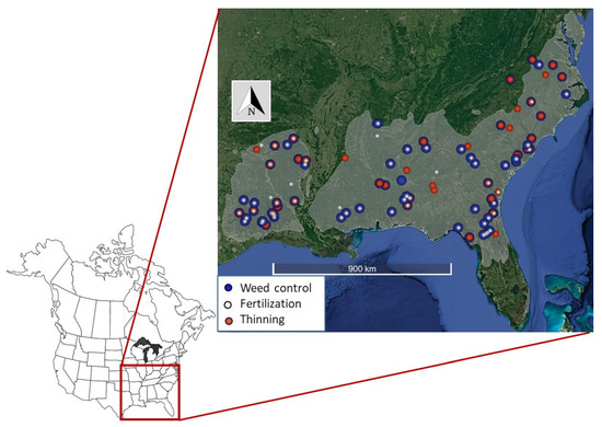
Figure 1.
Location of experimental loblolly pine plantations in the southeastern United States with symbols identifying sites with one of three primary silvicultural treatments (fertilization, weed control, and thinning). Multiple treatments at a site denoted with symbol overlap. The gray shaded area is the estimated natural distribution of loblolly pine [21].
2. Methods
2.1. Experimental Design
We sampled ecosystem C pools in 106 experiments located in loblolly pine plantations established across the SE US (Figure 1). The experiments were installed by several regional forestry research cooperatives between 1984 and 2009 [3]. The silvicultural treatments included fertilization (F), competing vegetation or ‘weed’ control (W), and thinning (T) and were applied at an experimental site alone or in combination. Treatments compared within a site, e.g., ‘Thinned vs. No Thinned’ (T vs. No T), were treated as a category and considered a single replicate. Typically, the comparisons included additional treatments (e.g., T vs. No T plus weed control or T vs. No T (+W)). In addition to comparisons of single silvicultural activities, some sites had comparisons of silvicultural intensity (i.e., differing types, frequency, and amounts of herbicide and fertilizer). Although treatments were often replicated with multiple plots at a site, only a single replicate for each treatment was measured as resources were focused on capturing many sites and elucidating the potential regional response to silviculture. Information on land use or silviculture prior to the experiment installation was lacking for most research plots. The average replicate plot size was 0.2 hectares. In total, 322 plots were sampled, beginning in the summer of 2012, with field sampling completed in the spring of 2015.
The average age of the plantations was 17 years (Table 1) at the time of measurement, which was past the midpoint to the common harvest age (~25–30 years) of intensively managed pine plantations in the region. Weed control typically began 1–2 years after planting, and was in some cases repeated until understory plants were effectively eliminated (e.g., ‘high’ intensity treatments). For the thinned treatments, the time since removal of trees was typically ~4 years prior to our sampling. A detailed description of plantation metrics by treatment is found in Appendix A.

Table 1.
Experimental plot metrics for age (years), quadratic mean diameter (QMD; cm) at 1.37 m, basal area (BA; m2 ha−1), tree density (TPH, trees ha−1), and site index (SI) across all treatment combinations.
Across fertilized plots, nitrogen (N) and phosphorus (P) were always added, while other elements were less consistently used (Table 2). The average accumulated N and P amounts applied were 373 kg ha−1 N and 59 kg ha−1 P at the time of sampling, more than the typical amounts (224 N kg ha−1, 28 P kg ha−1) added to regional plantations [3]. Fertilization mixtures varied across comparisons (Table 2), reflecting the diverse experimental objectives of the cooperatives installing the studies and perceived background fertility issues. High and low ‘intensity’ experiments differed by the amount or number of macronutrients in the fertilizer, and whether micronutrients were included (Table 2).
Table 2.
Cumulative elemental fertilization amounts (kg ha−1) for the fertilized plots found in the fertilization vs. no fertilization (F) comparisons (e.g., F vs. No F) and background fertilization for comparisons involving thinning (T) or competing vegetation or weed control (W) combinations (e.g., W vs. No W (+F)).
The mean annual precipitation ranged from 1100 mm year−1 to 1590 mm year−1 and mean annual air temperature from 13.5 to 20.3 °C for the 1980–2010 period [11]. Based on soil survey mapping, the greatest percentage of research sites was found on the Ultisols (61%) soil order, followed by Alfisols (23%), Spodosols (12%), Entisols (2%), and Inceptisols (2%) [11]. The predominant forest type of the study area is warm temperate forest with dominant competing vegetation varying across the region. Common early herbaceous competitors are grass species in the Andropogon and Panicum genera. In Florida and elsewhere along the lower Coastal Plain, saw palmetto (Serenoa repens (W. Bartram) Small) and gallberry (Ilex glabra (L.) A. Gray) are common shrub competitors with pine, and in the western region, yaupon (Ilex vomitoria Aiton) often forms dense thickets. A hardwood tree competitor common to all regions is sweetgum (Liquidambar styraciflua L.), with other hardwood tree species locally important as competitors [22].
Tree diameter at breast height (1.37 m; dbh), subsampled tree heights, and tree density (trees per hectare) were monitored by each research cooperative. Tree measurements generally occurred biannually and were <4 years from soil sampling measurements. From the dbh measurements, generalized allometric equations were used to calculate pine biomass C, with the equation including all aboveground tissues, bark, the root collar, and coarse roots ≥ 5 mm in diameter [23]. The C concentrations of tree biomass components were assumed to be 50% [24]. Tree height and plantation age (AGE) were also used to estimate site index (SI), which is a projection of the height of a tree to a reference age (25 years for loblolly pine). The equations from Dieguez-Aranda et al. [25] were used for realized SI estimates, or the SI created by pine genetics and silviculture interacting with site characteristics.
2.2. Sample Collection for Ecosystem C Pools
Each experimental plot was sampled in eight randomly selected locations to quantify the C in the understory plants, coarse woody debris (CWD), and organic and mineral soil layers. If a random location was <0.25 m from the base of a tree, then another random point was selected to avoid large roots dominating a sample or impeding soil coring. Understory plants were clipped from within a 100 cm × 100 cm area, and any tree other than planted pine that was >2.5 cm at DBH was measured and the tree species identified. Biomass was estimated for these non-pine trees with a species-specific allometric equation [26]. From within this 100 cm × 100 cm area, a centered 30 cm × 30 cm area was used to estimate CWD. CWD with a base diameter > 7.5 cm and located inside the plots was measured for its length to the first break, and then the diameter at the outside end measured. Rules for tallying CWD by splits or decay classes followed those of the Forest Inventory and Analysis (FIA) and the equations created by FIA used to estimate CWD mass and C [27]. Fine woody debris (<7.5 cm), and pine and root litter was included in the surface organic layer (Oi, and Oe + Oa [28]) estimates, and all were collected within a 30 cm × 30 cm frame. The Oi was initially separated from the Oe + Oa layers to facilitate laboratory processing. The two layers were summed and treated as a single unit, hereafter referred to as the soil organic layer.
From the center of these same locations, mineral soil was collected for fixed depth intervals: 0–10, 10–20, 20–50, and 50–100 cm. Four of the organic and mineral soil samples were randomly assigned to one of two subgroups, consolidated, and processed in bulk. For 1.9% of soil cores, a full depth interval could not be extracted because rocks or an impenetrable soil layer prevented soil coring through the entire interval. When this occurred and if another location was retrieved, the bulk density of the soil profile and soil C concentration were used to estimate soil C amounts. For three sites, none of the cores could be retrieved to depths > 20 cm and these were removed from the soil analysis.
The bulked soil and organic layer samples were mixed until homogenized, and then a subsample pulled that was equivalent to ~10%–20% of the total mass for the 20–50 cm and 50–100 cm layers. For the 0–10 cm and 10–20 cm layers, typically 100% of the total mass was processed. The soil was passed over a 2 mm sieve to remove live roots, detritus, and rocks. The live roots from this sample were separated into the size classes: 2–5 mm, 1–2 mm, and <1 mm. Roots > 5 mm were removed from the soil sample and not counted as a separate root mass estimates as this size fraction was captured by the total tree estimates [23]. Soil detritus (e.g., fragmented bark and wood, dead roots, char) within the mineral soil was also estimated from this subsample.
Roots and detritus were washed in deionized water, dried at 65 °C for at least 48 h, and weighed. The C concentration of roots and soil detritus was assumed to be 50% [19]. The organic and mineral soils were ground in roller mills or with mortar and pestle, and then analyzed for elemental C and N concentrations in duplicate using dry combustion elemental analyzers (CE Elantech (Lakewood, NJ, USA) NC 2100 analyzer; Flash EA 1112 (Milan, Italy) ThermoElectron; Elementar (Hanua, Germany)). Bulk density was directly estimated for the mineral 0–10 cm and 10–20 cm layers using a bulk density sampler. For mineral soils > 20 cm depth, 54% of the soil intervals were directly estimated for bulk density, and modeling (pedo-transfer and random forest approach) was used to estimate the remainder [11].
In some locations, field crews tallied ~10–50 cm tall tree stumps but their contribution as a distinct C pool was not estimated because of their inconsistent geometric form (Appendix B). Because the stumps were often well above the ground surface (an unusual practice in modern harvesting), we speculate that they may have been residual from the initial harvest of the region’s primary pine or hardwood forest. The silvicultural practices we examined were unlikely to have differentially affected the current mass of these stumps. In total, 2359 stumps ranging in diameter from 2–65 cm were tallied across all plots.
3. Data Analysis
A paired plot analysis was conducted on all pools (PROC TTEST, SAS version 9.4). Each site having a valid comparison for a category (e.g., F vs. No F (+W)) was treated as a replicate. The comparisons were tested for normality and outliers. While examining relatively small C pools (understory, roots < 5 mm, soil detritus, and CWD), Q-Q plots indicated these pools were non-normal and contained many zero values and outliers. Rather than explore transformation options for categories typically representing ~1% of total C, these pools were added to either pine biomass (added understory biomass and roots < 5 mm) or the soil organic layer (added soil detritus and coarse woody debris) for analysis. From these groupings, new categories were created: Vegetation C and detritus C pools. Both combined pools passed Q-Q visual checks for normality. For the pools within the mineral soil horizons, a Holm correction was used to adjust p-values for the multiple comparisons with depth intervals for a given contrast in treatments [29]. The number of plots or replicates varied among treatment comparisons (Appendix C and Appendix D). All mean values are followed by ±standard error.
A general linear model selection procedure (GLMSELECT, SAS version 9.4), a flexible model selection module, was used to evaluate response models for the detritus and detritus + vegetation pools of C. Independent variables were tested that are typically known or monitored by plantation managers: AGE, SI, and TPH. Models were selected using the LASSO (least absolute shrinkage and selection operator) procedure with iterative testing of parameters [30], and parameter selection stopped when the variable combinations minimized the Mallow’s C(p) Criterion [31]. Cook’s D statistic was used to determine leveraged points, which were removed if the statistic > 3 × µ. The data used in the analysis are found in the Supplementary Material.
4. Results
4.1. C Pools
Among all ecosystem C pools, the greatest amount of C was found in the mineral soil to 100 cm (79.8 ± 4.6 Mg C ha−1), with a range of 20.4–260.0 Mg C ha−1 across all evaluated stands (Figure 2A). Closely following the mineral soil was the amount of C in live pine biomass (79.2 ± 4.3 Mg C ha−1), with a range of 7.1–187.8 Mg C ha−1 (Figure 2A). Together these two pools contained 90% of the ecosystem C in the sampled plantations. The next largest pools were the surface soil organic layers (range = 1.6–37.1 Mg C ha−1, average = 11.3 ± 0.9 Mg C ha−1) and the roots < 5 mm found throughout the soil profile (range = 0.15–65.8 Mg C ha−1, average = 4.7 ± 0.6 Mg C ha−1) (Figure 2B). The C in tree biomass, soil organic layers, and roots < 5 mm together accounted for ~54% of the ecosystem C and the mineral soil C was ~45%. The remaining C in vegetation and detritus pools—understory aboveground biomass, soil associated debris and surface woody debris, were on average less than 0.35% of ecosystem C but relatively large estimates (>5 Mg C ha−1) were occasionally measured for each pool (Figure 2C). For soil detritus, stump debris or char were often the source of these observations. For understory C, relatively high values occurred when hardwoods reached the mid-canopy.
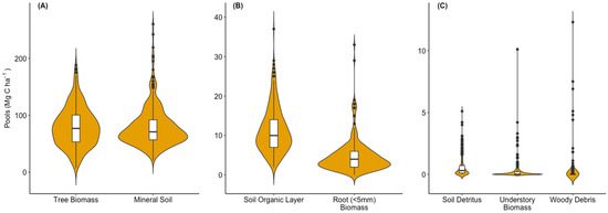
Figure 2.
Violin plots showing the interquartile range (white box, vertical line is 1.5 × range), median (cross bar), and probability density function (shaded area) of the C distribution among pools of (A) tree biomass and mineral soils to 100 cm, (B) soil organic layers and live roots, and (C) soil detritus, understory biomass and woody debris across the managed loblolly pine plantations. Note the Y-axis scale decreases from panel A to C and that extreme outliers are not included for some categories so that the probability density functions are fully visible.
4.2. Comparisons between Treatments
When comparing paired treatments, there was no effect of any silvicultural treatment on soil C for any mineral soil depth interval (Appendix C), or for the total amount of C in the 0–100 cm profile (Figure 3). Although not significant (p = 0.132), the largest observed difference was for the T vs. No T (+W) contrast, where soil C from 0–100 cm in thinned plots was 82.2 ± 4.2 compared to 111.9 ± 5.9 (No T) Mg C ha−1 in unthinned plots (Appendix A Table A2). This treatment comparison had the lowest number of replicates (n = 7), and second greatest overall soil C relative to the other treatments (Appendix C). The largest average mineral soil C was observed for the F vs. No F (+W) contrasts (113.0 Mg C ha−1 across treatments, n = 9), and the smallest for the W vs. No W (+TF) (57.6 Mg C ha−1 across treatments, n = 11) (Appendix C). This highlights that the comparisons were unevenly distributed across the background variation in soil C that is caused by edaphic conditions and soil mineralogy [11].
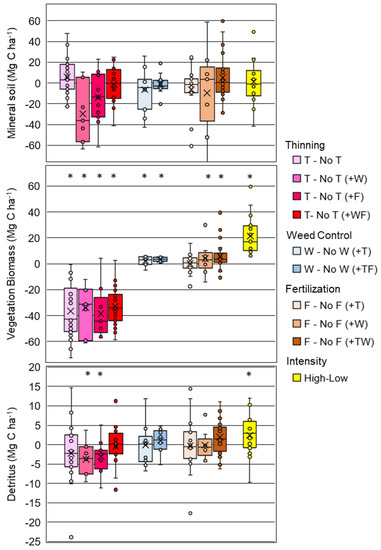
Figure 3.
Box plots (x = mean, line = median) of treatment differences (e.g., F-No F or F vs. No F) for the mineral soil to 100 cm (top panel), vegetation biomass (mid panel) and detritus (bottom panel) for comparisons of thinning (T), weed control (W), fertilization (F), and high versus low management intensity treatments. Additional treatments applied across both plots in a contrast are in parentheses (e.g., (+TF)). The (*) indicates a significant contrast.
Several silvicultural comparisons indicated significant changes in vegetation C (pine + roots < 5 mm + understory). Thinning consistently reduced vegetation C (p < 0.05) for all treatment combinations (Figure 3), resulting in thinned plantations having on average 35.5 ± 1.2 Mg C ha−1 less vegetation C than unthinned. Weed control in both thinned (+T) and thinned and fertilized (+TF) plantations increased the C in vegetation 3.3 ± 1.2 Mg C ha−1 (p < 0.05) (Figure 3, Appendix D). On average, fertilization significantly increased (p < 0.05) vegetation by 4.0 ± 1.2 Mg C ha−1 for plots receiving weed control (+W), and by 5.7 ± 2.3 Mg C ha−1 for the plots receiving both thinning and weed control (+TW) treatment combinations (Appendix D). The high intensity treatments increased the C in vegetation (108.6 ± 6.5 Mg C ha−1) relative to the low intensity treatments (87.2 ± 5.6 Mg C ha−1) (p < 0.05) (Appendix D).
Only three silvicultural treatment combinations significantly (p < 0.05) changed the detrital C pool (soil organic layer + coarse-woody debris + soil detritus): T vs. No T (+W), T vs. No T (+F), and the high vs. low intensity comparisons (Figure 3). Thinning in weed control treatments decreased detritus by 3.8 ± 1.1 Mg C ha−1 (T vs. No T (+W) and in fertilized treatments it was decreased by 3.0 ± 1.9 Mg C ha−1 (T vs. No T (+F)) (Appendix D). Among all treatment combinations, the two intensity contrasts had the greatest detritus values (high = 18.2 ± 1.6 Mg C ha−1, low = 16.6 ± 1.8 Mg C ha−1, Appendix D), with a significantly (p = 0.037) greater amount in the high intensity treatments (one outlier removed; Figure 3).
4.3. Models of C Pool Dynamics
The fitted statistical models included interactions among SI, AGE, and TPH (Table 3). For the detritus pools, all positive parameters were found with the model including TPH × SI, and TPH × SI × AGE with a negative intercept (Table 3). Two points of estimated detritus were identified as having high leverage on the model and were removed from the analysis (not shown). The final model for detritus explained 29% of the variance (Figure 4, Table 3). For the detritus + vegetation model, there were no outliers or leverage points identified. The intercept and parameters for AGE and AGE × SI × TPH were negative in the model, while SI × Age and TPH × SI were positive (Figure 4, Table 3). The model explained 87% of the variance in the data. An initial run of both models showed the residuals tended toward heteroscedasticity, but a natural log transformation of TPH removed this effect. Models of mineral soil C trends were not explored with these variables as the paired plot analysis, by depth or in aggregate (0–100 cm), did not suggest silviculture was affecting soil C pools.
Table 3.
Models describing the relationships between detritus and vegetation C (Mg C ha−1) and site index (SI), trees per hectare (TPH), and stand age (AGE) across loblolly pine plantations. Models were selected based on the step decrease in Mallow’s C(p) statistic. TPH was natural log transformed in the model and all plantations were older than 4 years.
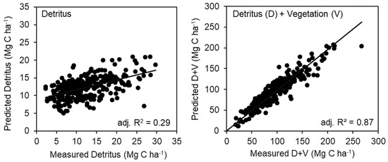
Figure 4.
The regression model results presented as measured versus predicted values for (left panel) detritus and (right panel) detritus plus vegetation (D + V). Two points in the detritus model were deemed high leverage (Cook’s D statistic) and removed from the analysis.
5. Discussion
This study reflects the most comprehensive assessment of the effects of silvicultural treatments on pine plantation C pools in the SE US. While the response of tree biomass C to silvicultural practices are well-known for some management treatments (e.g., thinning) across many forest types [32], few North American forests receive as great a diversity in the types of intensive silvicultural treatments as the pine plantations of the SE US [3]. Our results show that: (1) thinning reduces the C in vegetation and detritus (where fertilization or weed control are added independently); (2) fertilization increases vegetation C where weed control is also applied; when both are applied at higher levels, vegetation and detritus C can be further increased; and (3) weed control increases vegetation C but it does not affect detritus C. We note that the absolute change in the mass of these C pools would likely vary with site factors (e.g., climate, stand age) [33,34], tree characteristics unmeasured in this study (e.g., pine genetics) [35], intensity of silvicultural treatments [36], and years since treatment [37]. Therefore, the significant effects (Figure 3) should not be used to generalize about the magnitude of C pool response to silvicultural applications. Rather, the regression models (Table 3) combined with direct measurements (AGE, SI, and TPH) may be better able to capture how silvicultural practices or stand development affect detritus and vegetation C pools.
We created an empirical model so that landowners can easily estimate these C pools (Table 3), as opposed to using the data to validate a mechanistic process model of tree physiological function or decomposition processes as these generally require greater user sophistication [33]. Unlike mechanistic or growth and yield models [38], this approach limits our ability to infer causality and project future C storage conditions; nonetheless, we expect the effects of most silvicultural treatments are reflected in their influence on either TPH (e.g., thinning, planting density) or on SI (e.g., fertilization, weed control) [34]. In addition, since the study sites were distributed across nearly the entire natural range of loblolly pine, the model reflects regional disturbance processes and gradients in climate and soil conditions. For example, the TPH parameter captures the effects of thinning but also that of initial planting density, self-thinning, or regional mortality events (e.g., beetle outbreaks, ice storms). Across climatic or soil gradients, the SI of loblolly pine plantations is greater in warmer and wetter climates [39,40,41], where soil nutrient availability is greater [42], and where variation in the depth to the water table either negatively or positively affects tree growth [43]. For silvicultural treatments, fertilization tends to increase SI whenever nutrients are growth limiting and/or competing vegetation is controlled [34,36]. Importantly, SI might capture complex relationships among silvicultural treatments. For example, fertilization without weed control in thinned stands resulted in no increase in the C stored in vegetation (Figure 3) and no increase in SI (not shown). The ineffectiveness of moderate fertilization to increase pine biomass where there is an intact understory has been previously reported for pine plantations in the region [44], and likely reflects that several understory species are highly effective competitors for nutrients [22,45].
Both TPH and SI could be managed to increase ecosystem C storage, but the relative effects of each variable differed substantially across the range of measured values in this study. We illustrate this using the statistical models and the averages of SI (planting TPH held constant) and planting TPH (SI held constant) for each third of the measured values (Figure 5A–D). A model of self-thinning was used to estimate how TPH may change up until age 29 given the fixed SI or planting TPH [38]. An SI change from 20.7 to 26.8 corresponded to an increase in detritus + vegetation accumulation of 70.9 Mg C ha−1 (Figure 5A) and for detritus of 6.0 Mg C ha−1 (Figure 5B) by age 29 years (initial planting density = 1500 TPH) in unthinned stands. For an increase in planting density from 750 to 3000 trees ha−1 (average SI = 23.4), the increase for detritus + vegetation was 42.0 Mg C ha−1 (Figure 5C) and 3.0 Mg C ha−1 for detritus (Figure 5D) at age 29 years. The relative effect of planting TPH on C accumulation is considerably lower than that of SI. Given the error in these equations (Table 3), significant (p < 0.05) changes in pools would be detected when a loss or gain occurred of 4.9 Mg C ha−1 in detritus or 26.2 Mg C ha−1 in the detritus + vegetation pools, requiring rather large changes in SI, TPH, or plantation age for detection. Although the SI and TPH could be optimized together to maximize C storage, we note that controlled experiments and modeling indicate that increased stand density can depress SI in loblolly pine plantations [46], highlighting that tradeoffs will likely occur between these two factors.
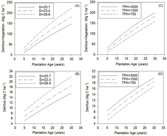
Figure 5.
(A–D) Modeled estimates of detritus + vegetation and detritus pools with plantation age for the average of the upper, mid, and lower thirds (A,B) for site index (SI) values at a fixed initial planting density of 1500 trees per hectare (TPH), and (C,D) varying initial planting densities at a fixed SI = 23.4.
The models captured the well-known slowing rate of C accumulation in vegetation and detritus as forests mature [47] (Figure 5A–D), but across all measured plantations, the age or degree of stand development did not correspond to a clear asymptote for these pools. This is a common observation in the pine plantations of the SE US as they generally continue to accumulate C up to the point of harvest age (~25–35 years) [48,49,50]. Given the investments in seedling genetics, planting, and early care in plantations [51], it would likely be unprofitable to allow stand development to proceed until tree mortality and decomposition exceeds or equals forest growth (i.e., peak C storage). A plantation’s approach toward peak C storage would likely accelerate with pine growth (i.e., SI) [34,47], and although we cannot identify this peak without repeated measures through time, we illustrate the potential tradeoff between SI and AGE with two subgroups of high C storage plantations (>190 Mg C ha−1 detritus and vegetation) in our dataset (Supplementary Material). One group (n = 3) was among the oldest plantations at age 27 years and had accumulated 230.9 ± 18 Mg C ha−1 with an average SI of 25.0 ± 0.1. Another group was younger (age = 18, n = 6), had an average SI of 29.1, and had accumulated 199.2 ± 0.1 Mg C ha−1. Thus, even with a 15% greater SI than the older stands, there may be the potential for continued C accumulation in the younger stands as they mature. Whether the plantations with greater SIs continue on a C accumulation trajectory toward the older stand’s C storage or toward a greater endpoint should be an area of active research as increasing rotation age has been identified as a potential way to increase landscape C storage in managed forests [39,52].
5.1. Mineral Soil C
Our assessment indicates that despite forest management effects on soil nutrient capital (e.g., fertilization), species composition (e.g., weed control), and forest biomass (thinning, intensity), there was no discernible effect on mineral soil C storage. Although this regional analysis incorporates a notable amount of variation in inherent mineral soil C [11], our non-significant results agree with case studies on Spodosols examining the effects of fertilization and weed control on mineral soil C [20], and the intensity of management [37]. Deeper mineral soils have shown depressed soil C with long term weed control in a Spodosol [19], and surface (0–10 cm) mineral soil C in an Entisol and two Ultisols also indicated a decrease in soil C from weed control [53]. Echeverria et al. [54] found for loblolly pine stands on Ultisols and Spodosols a reduction in mineral soil C caused by weed control for the 0–10 cm layer. Another study on Spodosols found weed control reduced soil C in the spodic horizon and subsequently the soil to 100 cm in a slash pine (Pinus elliottii) plantation, but there was no effect of fertilization [18]. Sartori et al. [55] examined more soil depths (0–10, 10–30, 30–50 cm) on Ultisols and reported no trend in soil C with fertilization, while one soil layer (10–30 cm for one of three sites) decreased with weed control. Harding and Jokela [56] found that to a depth of 91 cm, organic matter in an Inceptisol was unresponsive to two different fertilization mixtures. In summary for these previous studies, fertilization has shown no effect but weed control has caused some losses, although we did not detect a response to this latter silvicultural practice here. Notably these past studies did not include as soil C the live or dead roots, and similarly we did not include as soil C the recently killed dead coarse roots associated with thinning (discussed in Section 5.2 below).
These observations are region specific, but studies from other cool and warm temperate forests suggest that mineral soil C storage is unaffected by thinning [32,57], and understory control [58]. However, a universal limitation to studies of soil C response to management is the difficulty in making accurate measurements [59]. Although there are some laboratory analytical procedures that can introduce measurement error, most difficulties in measuring soil C pools arise from the inherent vertical and horizontal complexity of soils, which is for example, a pronounced feature of Spodosols in the SE US (Appendix E). Soil C pools generally need to be highly responsive to management to detect changes [59], but the mineral soil C to 100 cm depth in the region has an average age of 1000–2000 years [60], suggesting a low level of turnover for the majority of soil C. Rather than measuring the response of soil C pools, estimates of root or microbial fluxes are often used to infer soil C dynamics under different forest management regimes.
Past studies on the primary mechanisms that affect soil C storage, heterotrophic respiration and organic matter deposition, do not suggest consistent patterns in the region’s pine plantations. For example, in response to fertilization, decomposer activity has increased [61,62], heterotrophic respiration has remained unchanged [63,64,65], or has been both stimulated and suppressed depending on the combination of added nutrients (N, P, Cu, Mn), the time since nutrient addition, and past silviculture [66]. Notably, most nutrients regularly added (e.g., N, P, K, Ca, Mg, B) in fertilizer mixes for southern pine [67] have not been tested for their effects on in situ decomposition processes or organic matter deposition either alone or in representative fertilizer mixtures. Where the C in tree biomass and detritus has been increased through the intensity of fertilization and weed control, past research found no discernible effect on soil C (0–30 cm) despite a ~55% increase in vegetation and detritus pools [37], potentially because belowground C allocation to fine roots decreased with fertilization intensity [35]. In contrast, other studies have found increases in coarse [68] and fine roots [69] where silviculture increased pine growth. Weed control has been found to decrease microbial activity [18] and the C in soil density fractions, but then have no effect on total soil C [70]. Previous studies’ lack of consistent response of these fluxes to management, combined with the narrow range of plantation conditions measured in past studies, may mean that our ‘non-response’ of soil C is a manifestation of the inherent spatial and temporal complexity of root and microbial processes.
5.2. Unmeasured C Pools
We attempted to account for all ecosystem C pools in this assessment but post-thinning residuals as treetops and stumps posed difficulties in terms of accurate measurement. During thinning in plantations, trees are felled and often hauled to a central processing location where the merchantable stems are loaded onto trucks. Although some branches are broken during felling and transit (and potentially captured by our methods), most of the treetop is cut from the merchantable stem at the central processing location. After removing treetops, harvesters may then pile and leave them, burn them after piling, or sell the wood wastes for bioenergy while spreading the tree foliage back onto the site. We did not account for these fates as locating piles or ascertaining the outcome of waste handling was beyond this study, but it is estimated that treetops could account for ~10%–15% of total tree biomass C at the time of thinning [19]. Stumps created during thinning were also not measured if their structural integrity resisted penetration by soil corers. Tree cutting now occurs at the soil surface in these plantations, so modern stumps are often covered by litterfall, making them difficult to locate and measure. When decomposed enough to be sampled by soil coring, the stumps contributed to the soil detritus estimates. At the time of thinning, stumps and associated coarse roots could represent ~15%–30% of total live tree C [47]. For both the treetop and stump pools, the actual difference between thinned and unthinned forest C will be lower than we estimated at the time of harvest, and then change further with the time since harvest as the detrital wood decomposes in the thinned forests. Managers wishing to estimate the size of these C pools in situ could model their fates with published estimates of wood decomposition [71], but we caution that the larger stumps created by an end-of-rotation harvest may follow a different decomposition trajectory from the smaller ones created during thinning [72,73]. Regional FIA estimates of plantation C storage may also have difficultly capturing the dynamics of these pools because of their ‘low-profile’ (e.g., stumps) or non-random distribution (e.g., piles) [74].
5.3. Management Implications
Our results show how the rate of C accumulation can be increased in plantations (Figure 5A–D), with the statistical models serving as easily applied tools for assessing the effects of SI or TPH manipulation. However, for management to affect plantation C storage across rotations or the landscape, consideration may be required for potential tradeoffs with economic returns [75]. For example, increasing SI could reduce the time that a plantation needs to replace the C lost during the previous harvest [48], but it would also likely lower the age at which a profitable harvest could occur [76]. Modeling suggests that harvesting at a younger stand age can offset increased C accumulation over multiple rotations, resulting in little net gain in C [47,77]. Extending rotation age could increase landscape C storage, but to offset a loss in economic returns to a landowner, then payment for C sequestration may be needed [78]. These C payments should be sensitive to verification of in situ storage [79], and so we note that the stand metrics used in our regression models can all be detected with remote sensing techniques that measure pine heights for site index, stand density, and the time since the last harvest c.f. [80].
Our results suggest that for the SE US overall, common silvicultural practices have no consequential effect on mineral soil C. However, we urge caution in applying this finding to silvicultural practices not examined here or for specific soil types. In particular, extremely high soil C densities (>200 Mg C ha−1) occur in the poorly drained soils along the lower coastal plain of the region [11]. An approach to improving pine growth in these soils is to reduce soil moisture by facilitating drainage [51], which would very likely increase heterotrophic respiration and potential soil C loss as oxygenation levels increase in the soil profile. Conversely, we found many plots in the Piedmont (primarily Ultisol soil order) areas of the SE US with very low soil C concentrations (<60 Mg C ha−1) [11], potentially because of past agricultural practices that reduced C inputs and caused soil erosion [81,82]. Afforestation with pine plantations managed for accelerated growth on these soils may increase overall mineral soil C storage [6]. With the past land use mostly unknown for these sites, it is possible that this factor could have influenced our results.
6. Conclusions
This study highlights how C storage in vegetation and detritus pools can be influenced by silviculture in loblolly pine plantations. Landowners recording the plantation metrics of site index, plantation age, and tree density can generate their own estimates of these C pools, and if silviculture influences these metrics, the landowner can estimate C pool response to silviculture. Importantly, remote sensing could extract these metrics and allow land managers to use them in remote verification of C storage in detritus and vegetation biomass. We note that the C stored in post-harvest stumps and piled treetops is not estimated in this study and so we have underestimated plantation C storage and may have overestimated the reductions in ecosystem C caused by thinning because we did not track these pools after a harvest. Following how harvesters handle treetops or applying models of decomposition could be used to estimate the dynamics of both piles and stumps in situ. Notably, large and seemingly old stumps persist across the SE US, suggesting that more research is needed concerning their contribution to long-term regional C dynamics. At the scale of loblolly pine’s natural distribution, mineral soil C appears unresponsive to the silviculture practices examined in this study. At the scale of a stand or sub-region, especially those regions with relatively high or low amounts of background soil C, the potential for soil C losses or gains in response to silviculture warrants additional experiments that simultaneously measure root and microbial processes.
Supplementary Materials
The following supporting information can be downloaded at: https://www.mdpi.com/article/10.3390/f13010036/s1.
Author Contributions
Conceptualization; data curation; formal analysis; funding acquisition; investigation; methodology; project administration; resources; software; supervision; validation; visualization; J.G.V., writing—original draft, formal analysis, conceptualization; R.B., formal analysis, data curation, writing—review & editing; M.A., investigation, methodology; R.A., data curation, resources; A.B., formal analysis, writing—review & editing; H.E.B., conceptualization, data curation, resources, writing—review & editing; C.A.G.-B., formal analysis, writing—review & editing; S.G., methodology, writing—review & editing; E.J.J., methodology, writing—review & editing; M.B.K., funding acquisition; M.A.L., investigation, methodology; D.M., conceptualization, writing—review & editing; T.A.M., funding acquisition, methodology, project administration; C.M., investigation; C.W.R., data curation, investigation; R.E.W., supervision, methodology, writing—review & editing; T.R.F., project administration, conceptualization, supervision, writing—review & editing. All authors have read and agreed to the published version of the manuscript.
Funding
This research was a part of the Pine Integrated Network: Education, Mitigation, and Adaptation project (PINEMAP), a Coordinated Agricultural Project funded by the USDA National Institute of Food and Agriculture, Award #2011-68002-30185.
Data Availability Statement
The estimated C values used for this study are found in the Supplementary Material. Additional metadata are available upon request.
Acknowledgments
Dozens of undergraduate and graduate students, technicians, and visiting scientists assisted in the collection and processing of field samples. We are deeply indebted to them for their hard work and diligence. We acknowledge the financial and logistical support provided by the member companies associated with the research cooperatives. Salvador Gezan provided early statistical advice.
Conflicts of Interest
The authors declare no conflict of interest.
Appendix A
Table A1.
The average ((±stderr) tree density (trees per hectare (TPH)), site index (no units, (SI)), stand density index (no units, (SDI)), and plantation age (years) for different treatments alone (competing vegetation or ‘weed’ control (W), thinning (T), fertilization (F)) or in combination (e.g., Thinning + Competition control (TW)).
| Treatment | TPH | SI | SDI | Age |
|---|---|---|---|---|
| Control | 1221 ± 75 | 21.9 ± 0.3 | 773 ± 38 | 18 ± 1.2 |
| W | 1160 ± 52 | 23.1 ± 0.9 | 690 ± 83 | 15 ± 2.1 |
| T | 637 ± 76 | 22.2 ± 0.4 | 457 ± 29 | 19 ± 0.7 |
| TW | 461 ± 50 | 22.4 ± 0.5 | 406 ± 26 | 19 ± 0.7 |
| F | 1094 ± 94 | 22.0 ± 0.6 | 687 ± 60 | 20 ± 1.6 |
| FW | 1323 ± 109 | 23.7 ± 0.5 | 788 ± 43 | 18 ± 1.4 |
| FT | 553 ± 64 | 22.6 ± 0.4 | 423 ± 27 | 19 ± 0.8 |
| FTW | 495 ± 51 | 23.3 ± 0.3 | 440 ± 22 | 20 ± 0.6 |
| Intensity | ||||
| High | 1697 ± 93 | 26.9 ± 0.3 | 902 ± 25 | 14 ± 0.4 |
| Low | 1887 ± 191 | 25.8 ± 0.5 | 823 ± 50 | 14 ± 0.2 |
Appendix B

Figure A1.
Stump in the foreground from a forest before plantation establishment. Across the region, 2359 stumps were encountered but were not included in the forest carbon assessment (photo credit Andy Laviner).
Figure A1.
Stump in the foreground from a forest before plantation establishment. Across the region, 2359 stumps were encountered but were not included in the forest carbon assessment (photo credit Andy Laviner).

Appendix C
Table A2.
Mineral soil carbon (Mg C ha−1) average estimates (±stderr) for each contrast with number of sites (N) for each comparison. No comparison was significant for a depth interval and treatment, and the 0–100 differences are shown in Figure 3.
Table A2.
Mineral soil carbon (Mg C ha−1) average estimates (±stderr) for each contrast with number of sites (N) for each comparison. No comparison was significant for a depth interval and treatment, and the 0–100 differences are shown in Figure 3.
| Thinning (T) Comparisons | ||||||||
| Depth (cm) | T | No T | T (+W) | No T (+W) | T (+F) | No T (+F) | T (+WF) | No T (+WF) |
| 0–10 | 19.4 ± 1.3 | 19.5 ± 1.2 | 25.1 ± 4.3 | 27.4 ± 5.1 | 26.1 ± 4.3 | 26.4 ± 5.1 | 28.0 ± 2.2 | 29.4 ± 2.9 |
| 10–20 | 10.3 ± 0.6 | 9.7 ± 0.8 | 14.4 ± 3.2 | 21.1 ± 5.2 | 15.4 ± 3.2 | 14.4 ± 5.2 | 19.3 ± 2.6 | 19.7 ± 3.6 |
| 20–50 | 19.7 ± 2.3 | 16.6 ± 1.1 | 24.4 ± 6.1 | 32.6 ± 5.9 | 19.4 ± 6.1 | 25.6 ± 5.9 | 27.5 ± 2.6 | 29.0 ± 3.9 |
| 50–100 | 17.7 ± 2.3 | 15.5 ± 1.9 | 18.2 ± 3.3 | 30.6 ± 7.6 | 16.9 ± 3.3 | 25.7 ± 7.6 | 25.2 ± 4.3 | 23.2 ± 2.4 |
| 0–100 | 67.0 ± 1.6 | 61.3 ± 1.2 | 82.2 ± 4.2 | 111.9 ± 5.9 | 78.3 ± 4.2 | 92.2 ± 5.9 | 100.0 ± 3.0 | 101.3 ± 3.2 |
| N = 23 | N = 7 | N = 11 | N = 20 | |||||
| Weed Control (W) Comparisons | ||||||||
| Depth (cm) | W (+T) | No W (+T) | W (+TF) | No W (+TF) | ||||
| 0–10 | 17.7 ± 2.2 | 18.3 ± 2.3 | 17.9 ± 1.8 | 16.5 ± 1.2 | ||||
| 10–20 | 9.0 ± 1.2 | 8.9 ± 1.1 | 9.4 ± 1.2 | 9.7 ± 1.3 | ||||
| 20–50 | 15.9 ± 2.2 | 19.7 ± 3.9 | 15.0 ± 2.1 | 15.7 ± 2.0 | ||||
| 50–100 | 16.3 ± 2.2 | 18.5 ± 3.8 | 14.8 ± 2.4 | 16.3 ± 2.0 | ||||
| 0–100 | 58.9 ± 2.8 | 65.4 ± 2.0 | 57.0 ± 1.9 | 58.1 ± 1.6 | ||||
| N = 11 | N = 11 | |||||||
| Fertilization (F) Comparisons | ||||||||
| Depth (cm) | F (+T) | No F (+T) | F (+W) | No F (+W) | F (+TW) | No F (+TW) | ||
| 0–10 | 21.7 ± 2.0 | 23.7 ± 2.3 | 32.2 ± 4.3 | 29.6 ± 4.0 | 21.4 ± 1.6 | 19.7 ± 1.7 | ||
| 10–20 | 11.4 ± 1.2 | 11.5 ± 1.2 | 17.2 ± 1.7 | 18.4 ± 3.2 | 11.6 ± 1.3 | 10.6 ± 0.9 | ||
| 20–50 | 18.9 ± 1.8 | 21.4 ± 2.5 | 35.9 ± 6.9 | 31.7 ± 4.3 | 19.7 ± 2.1 | 19.7 ± 2.3 | ||
| 50–100 | 16.7 ± 1.5 | 18.5 ± 2.9 | 23.3 ± 2.9 | 38.8 ± 11.6 | 24.2 ± 3.8 | 21.8 ± 3.2 | ||
| 0–100 | 68.6 ± 1.6 | 75.2 ± 2.3 | 108.6 ± 3.9 | 118.4 ± 5.8 | 76.8 ± 2.2 | 71.7 ± 2.0 | ||
| N = 19 | N = 9 | N = 26 | ||||||
| Intensity Comparison | ||||||||
| Depth (cm) | High | Low | ||||||
| 0–10 | 22.9 ± 1.4 | 21.8 ± l.5 | ||||||
| 10–20 | 14.4 ± 1.0 | 14.0 ± 1.0 | ||||||
| 20–50 | 23.0 ± 1.9 | 23.6 ± 2.1 | ||||||
| 50–100 | 24.7 ± 5.1 | 25.4 ± 3.7 | ||||||
| 0–100 | 85.0 ± 2.4 | 84.8 ± 2.1 | ||||||
| N = 18 | ||||||||
Appendix D
Table A3.
Vegetation biomass and detritus (Mg C ha−1) average estimates (±stderr), the number of plots (N) and average plantation age (years) used for each comparison. Significant differences are shown in Figure 3 of main text.
Table A3.
Vegetation biomass and detritus (Mg C ha−1) average estimates (±stderr), the number of plots (N) and average plantation age (years) used for each comparison. Significant differences are shown in Figure 3 of main text.
| Thinning (T) Comparisons | ||||||||
| T | No T | T (+W) | No T (+W) | T (+F) | No T (+F) | T (+WF) | No T (+WF) | |
| Biomass | 64.4 ± 3.2 | 100.9 ± 4.6 | 64.1 ± 7.8 | 98.1 ± 11.6 | 64.5 ± 6.9 | 103.0 ± 10.6 | 75.3 ± 5.5 | 108.3 ± 5.5 |
| Detritus | 10.6 ± 1.2 | 12.9 ± 1.3 | 11.8 ± 1.8 | 15.6 ± 1.3 | 14.1 ± 2.0 | 17.1 ± 2.1 | 15.4 ± 1.6 | 15.8 ± 1.8 |
| Plots | N = 22 | N = 7 | N = 11 | N = 20 | ||||
| Age | 20 | 18 | 21 | 21 | ||||
| Weed Control (W) Comparisons | ||||||||
| W (+T) | No W (+T) | W (+TF) | No W (+TF) | |||||
| Biomass | 71.0 ± 4.8 | 68.7 ± 4.3 | 73.6 ± 4.8 | 70.4 ± 4.9 | ||||
| Detritus | 10.2 ± 1.4 | 10.3 ± 1.4 | 11.3 ± 0.9 | 10.2 ± 1.4 | ||||
| Plots | N = 10 | N = 10 | ||||||
| Age | 20 | 21 | ||||||
| Fertilization (F) Comparisons | ||||||||
| F | No F | F | No F | F | No F | |||
| (+T) | (+T) | (+W) | (+W) | (+TW) | (+TW) | |||
| Biomass | 63.8 ± 4.4 | 63.6 ± 3.6 | 70.6 ± 15.1 | 66.6 ± 14.3 | 63.8 ± 3.4 | 58.1 ± 3.7 | ||
| Detritus | 11.2 ± 1.2 | 11.0 ± 1.2 | 13.1 ± 1.5 | 12.9 ± 1.9 | 12.1 ± 1.2 | 10.1 ± 0.9 | ||
| Plots | N = 18 | N = 9 | N = 24 | |||||
| Age | 19 | 14 | 19 | |||||
| Intensity Comparison | ||||||||
| High | Low | |||||||
| Biomass | 108.6 ± 6.5 | 87.2 ± 5.6 | ||||||
| Detritus | 18.2 ± 1.6 | 16.6 ± 1.8 | ||||||
| Plots | N = 21 | |||||||
| Age | 14 | |||||||
Appendix E

Figure A2.
Typic Alaquod (Pomona series) to a depth of ~1 meter (to a grey Bt horizon) found in north Florida. Note the complex and wavy display of the dark Bh horizon (photo credit Allan Bacon).
Figure A2.
Typic Alaquod (Pomona series) to a depth of ~1 meter (to a grey Bt horizon) found in north Florida. Note the complex and wavy display of the dark Bh horizon (photo credit Allan Bacon).

References
- Pan, Y.; Birdsey, R.A.; Fang, J.; Houghton, R.; Kauppi, P.E.; Kurz, W.A.; Phillips, O.L.; Shvidenko, A.; Lewis, S.L.; Canadell, J.G.; et al. A Large and Persistent Carbon Sink in the World’s Forests. Science 2011, 333, 988–993. [Google Scholar] [CrossRef] [PubMed]
- Payn, T.; Carnus, J.M.; Freer-Smith, P.; Kimberley, M.; Kollert, W.; Liu, S.; Orazio, C.; Rodriguez, L.C.; Silva, L.N.; Wingfield, M.J. Changes in planted forests and future global implications. For. Ecol. Manag. 2015, 352, 57–67. [Google Scholar] [CrossRef]
- Fox, T.R.; Allen, H.L.; Albaugh, T.J.; Rubilar, R.; Carlson, C.A. Tree Nutrition and Forest Fertilization of Pine Plantations in the Southern United States. South. J. Appl. For. 2007, 31, 5–11. [Google Scholar] [CrossRef]
- McKinley, D.C.; Ryan, M.G.; Birdsey, R.A.; Giardina, C.P.; Harmon, M.E.; Heath, L.S.; Houghton, R.A.; Jackson, R.B.; Mor-rison, J.F.; Murray, B.C.; et al. A synthesis of current knowledge on forests and carbon storage in the United States. Ecol. Appl. 2011, 21, 1902–1924. [Google Scholar] [CrossRef] [PubMed]
- Favero, A.; Mendelsohn, R.; Sohngen, B. Using forests for climate mitigation: Sequester carbon or produce woody biomass? Clim. Chang. 2017, 144, 195–206. [Google Scholar] [CrossRef]
- Nave, L.E.; Domke, G.M.; Hofmeister, K.L.; Mishra, U.; Perry, C.H.; Walters, B.F.; Swanston, C.W. Reforestation can sequester two petagrams of carbon in US topsoils in a century. Proc. Natl. Acad. Sci. USA 2018, 115, 2776–2781. [Google Scholar] [CrossRef]
- Johnson, D.W.; Curtis, P.S. Effects of forest management on soil C and N storage: Meta analysis. For. Ecol. Manag. 2001, 140, 227–238. [Google Scholar] [CrossRef]
- Mayer, M.; Prescott, C.E.; Abaker, W.E.; Augusto, L.; Cécillon, L.; Ferreira, G.W.; James, J.; Jandl, R.; Katzensteiner, K.; Laclau, J.-P.; et al. Tamm Review: Influence of forest management activities on soil organic carbon stocks: A knowledge synthesis. For. Ecol. Manag. 2020, 466, 118127. [Google Scholar] [CrossRef]
- Koricheva, J.; Gurevitch, J. Uses and misuses of meta-analysis in plant ecology. J. Ecol. 2014, 102, 828–844. [Google Scholar] [CrossRef]
- Wear, D.N.; Greis, J.G. The Southern Forest Futures Project: Technical Report; Southern Research Station, Forest Service, U.S. Department of Agriculture: Asheville, NC, USA, 2013. [CrossRef]
- Ross, C.W.; Grunwald, S.; Vogel, J.G.; Markewitz, D.; Jokela, E.J.; Martin, T.A.; Bracho, R.; Bacon, A.R.; Brungard, C.W.; Xiong, X. Accounting for two-billion tons of stabilized soil carbon. Sci. Total Environ. 2020, 703, 134615. [Google Scholar] [CrossRef]
- Smith, J.E.; Domke, G.M.; Nichols, M.C.; Walters, B.F. Carbon stocks and stock changes on federal forest lands of the United States. Ecosphere 2019, 10, e02637. [Google Scholar] [CrossRef]
- Hoover, C.M.; Smith, J.E. Current aboveground live tree carbon stocks and annual net change in forests of conterminous United States. Carbon Balance Manag. 2021, 16, 17. [Google Scholar] [CrossRef]
- Han, F.X.; Plodinec, M.J.; Su, Y.; Monts, D.L.; Li, Z. Terrestrial carbon pools in southeast and south-central United States. Clim. Chang. 2007, 84, 191–202. [Google Scholar] [CrossRef]
- Albaugh, T.J.; Vance, E.D.; Gaudreault, C.; Fox, T.R.; Allen, H.L.; Stape, J.L.; Rubilar, R. Carbon Emissions and Sequestration from Fertilization of Pine in the Southeastern United States. For. Sci. 2012, 58, 419–429. [Google Scholar] [CrossRef]
- McKeand, S.E. The Evolution of a Seedling Market for Genetically Improved Loblolly Pine in the Southern United States. J. For. 2019, 117, 293–301. [Google Scholar] [CrossRef]
- Aspinwall, M.; McKeand, S.; King, J.S. Carbon Sequestration from 40 Years of Planting Genetically Improved Loblolly Pine across the Southeast United States. For. Sci. 2012, 58, 446–456. [Google Scholar] [CrossRef]
- Shan, J.; Morris, L.A.; Hendrick, R.L. The effects of management on soil and plant carbon sequestration in slash pine plantations. J. Appl. Ecol. 2001, 38, 932–941. [Google Scholar] [CrossRef]
- Vogel, J.G.; Suau, L.J.; Martin, T.A.; Jokela, E.J. Long-term effects of weed control and fertilization on the carbon and nitrogen pools of a slash and loblolly pine forest in north-central Florida. Can. J. For. Res. 2011, 41, 552–567. [Google Scholar] [CrossRef]
- Tumushime, I.; Vogel, J.G.; Minor, M.N.; Jokela, E.J. Effects of Fertilization and Competition Control on Tree Growth and C, N, and P Dynamics in a Loblolly Pine Plantation in North Central Florida. Soil Sci. Soc. Am. J. 2019, 83, 242–251. [Google Scholar] [CrossRef]
- Elbert, L.L., Jr. Checklist of United States Trees (Native and Naturalized); Ag. Handb. 541; Department of Agriculture: Washington, DC, USA, 1979; 375p.
- Neary, D.; Rockwood, D.; Comerford, N.; Swindel, B.; Cooksey, T. Importance of weed control, fertilization, irrigation, and genetics in slash and loblolly pine early growth on poorly drained spodosols. For. Ecol. Manag. 1990, 30, 271–281. [Google Scholar] [CrossRef]
- Gonzalez-Benecke, C.A.; Teskey, R.O.; Martin, T.A.; Jokela, E.J.; Fox, T.R.; Kane, M.B.; Noormets, A. Regional validation and improved parameterization of the 3-PG model for Pinus taeda stands. For. Ecol. Manag. 2016, 361, 237–256. [Google Scholar] [CrossRef]
- Johnsen, K.H.; Wear, D.N.; Oren, R.; Teskey, R.O.; Sanchez, F.; Will, R.E.; Butnor, J.; Markewitz, D.; Richter, D.; Rials, T.; et al. Carbon sequestration and southern pine forests. J. For. 2001, 99, 14–21. [Google Scholar]
- Diéguez-Aranda, U.; Burkhart, H.E.; Amateis, R. Dynamic site model for loblolly pine (Pinus taeda L.) plantations in the United States. For. Sci. 2006, 52, 262–272. [Google Scholar]
- Jenkins, J.C.; Chojnacky, D.C.; Heath, L.S.; Birdsey, R.A. National-scale biomass estimators for United States tree species. For. Sci. 2003, 49, 12–35. [Google Scholar]
- Woodall, C.W.; Monleon, V.J. Sampling Protocol, Estimation, and Analysis Procedures for the Down Woody Materials Indicator of the Fia Program; Northern Research Station, Forest Service, U.S. Department of Agriculture: Newtown Square, PA, USA, 2008. [CrossRef]
- Ditzler, C.; Scheffe, K.; Monger, H.C. (Eds.) Soil Science Division Staff. Soil Survey Manual; USDA Handbook Government Printing Office: Washington, DC, USA, 2017.
- Holm, S. A simple sequentially rejective multiple test procedure. Scand. J. Stat. 1979, 6, 65–70. [Google Scholar]
- Efron, B.; Hastie, T.; Johnstone, I.; Tibshirani, R. Least angle regression. Ann. Stat. 2004, 32, 407–499. [Google Scholar] [CrossRef]
- Hocking, R.R. The Analysis and Selection of Variables in Linear Regression. Biometrics 1976, 32, 1–50. [Google Scholar] [CrossRef]
- Ruiz-Peinado, R.; Bravo-Oviedo, A.; López-Senespleda, E.; Bravo, F.; del Rio, M. Forest management and carbon sequestration in the Mediterranean region: A review. For. Syst. 2017, 26, eR04S. [Google Scholar] [CrossRef]
- Thomas, R.Q.; Jersild, A.L.; Brooks, E.B.; Thomas, V.A.; Wynne, R.H. A mid-century ecological forecast with partitioned uncertainty predicts increases in loblolly pine forest productivity. Ecol. Appl. 2018, 28, 1503–1519. [Google Scholar] [CrossRef]
- Zhao, D.; Kane, M.; Teskey, R.; Fox, T.R.; Albaugh, T.J.; Allen, H.; Rubilar, R. Maximum response of loblolly pine plantations to silvicultural management in the southern United States. For. Ecol. Manag. 2016, 375, 105–111. [Google Scholar] [CrossRef]
- Drum, C.G.; Vogel, J.G.; Gezan, S.A.; Jokela, E.J. Belowground processes for two loblolly pine (Pinus taeda L.) families respond differently to the intensity of plantation management. For. Ecol. Manag. 2019, 441, 293–301. [Google Scholar] [CrossRef]
- Jokela, E.J.; Martin, T.A.; Vogel, J.G. Twenty-five years of intensive forest management with southern pines: Important lessons learned. J. For. 2010, 108, 338–347. [Google Scholar]
- Vogel, J.G.; He, D.; Jokela, E.J.; Hockaday, W.; Schuur, E.A. The effect of fertilization levels and genetic deployment on the isotopic signature, constituents, and chemistry of soil organic carbon in managed loblolly pine (Pinus taeda L.) forests. For. Ecol. Manag. 2015, 355, 91–100. [Google Scholar] [CrossRef]
- Gonzalez-Benecke, C.A.; Jokela, E.J.; Martin, T.A. Modeling the Effects of Stand Development, Site Quality, and Silviculture on Leaf Area Index, Litterfall, and Forest Floor Accumulations in Loblolly and Slash Pine Plantations. For. Sci. 2012, 58, 457–471. [Google Scholar] [CrossRef]
- Burkhart, H.E.; Brooks, E.B.; Dinon-Aldridge HSabatia, C.O.; Gyawali, N.; Wynne, R.H.; Thomas, V.A. Regional simulations of loblolly pine productivity with CO2 enrichment and changing climate scenarios. For. Sci. 2018, 64, 349–357. [Google Scholar] [CrossRef]
- Gonzalez-Benecke, C.A.; Teskey, R.O.; Dinon-Aldridge, H.; Martin, T.A. Pinus taeda forest growth predictions in the 21st century vary with site mean annual temperature and site quality. Glob. Chang. Biol. 2017, 23, 4689–4705. [Google Scholar] [CrossRef] [PubMed]
- Sabatia, C.O.; Burkhart, H.E. Predicting site index of plantation loblolly pine from biophysical variables. For. Ecol. Manag. 2014, 326, 142–156. [Google Scholar] [CrossRef]
- Subedi, S.; Fox, T.R. Predicting Loblolly Pine Site Index from Soil Properties Using Partial Least-Squares Regression. For. Sci. 2016, 62, 449–456. [Google Scholar] [CrossRef]
- Parresol, B.; Scott, D.; Zarnoch, S.; Edwards, L.; Blake, J. Modeling forest site productivity using mapped geospatial attributes within a South Carolina Landscape, USA. For. Ecol. Manag. 2017, 406, 196–207. [Google Scholar] [CrossRef]
- Jokela, E.J.; Martin, T.A. Effects of ontogeny and soil nutrient supply on production, allocation, and leaf area efficiency in loblolly and slash pine stands. Can. J. For. Res. 2000, 30, 1511–1524. [Google Scholar] [CrossRef]
- Subedi, P.; Jokela, E.J.; Vogel, J.G. Inter-Rotational Effects of Fertilizer and Herbicide Treatments on the Understory Vegetation Community in Juvenile Loblolly Pine (Pinus taeda L.) Stands. For. Sci. 2017, 63, 459–473. [Google Scholar] [CrossRef]
- Sharma, M.; Amateis, R.L.; Burkhart, H.E. Top height definition and its effect on site index determination in thinned and unthinned loblolly pine plantations. For. Ecol. Manag. 2002, 168, 163–175. [Google Scholar] [CrossRef]
- Gonzalez-Benecke, C.A.; Martin, T.A.; Jokela, E.J.; De La Torre, R. A Flexible Hybrid Model of Life Cycle Carbon Balance for Loblolly Pine (Pinus taeda L.) Management Systems. Forests 2011, 2, 749–776. [Google Scholar] [CrossRef]
- Aguilos, M.; Mitra, B.; Noormets, A.; Minick, K.; Prajapati, P.; Gavazzi, M.; Sun, G.; McNulty, S.; Li, X.; Domec, J.-C.; et al. Long-term carbon flux and balance in managed and natural coastal forested wetlands of the Southeastern USA. Agric. For. Meteorol. 2020, 288–289, 108022. [Google Scholar] [CrossRef]
- Bracho, R.; Starr, G.; Gholz, H.L.; Martin, T.A.; Cropper, W.P.; Loescher, H.W. Controls on carbon dynamics by ecosystem structure and climate for southeastern U.S. slash pine plantations. Ecol. Monogr. 2012, 82, 101–128. [Google Scholar] [CrossRef]
- Gholz, H.L.; Fisher, R.F. Organic Matter Production and Distribution in Slash Pine (Pinus elliottii) Plantations. Ecology 1982, 63, 1827. [Google Scholar] [CrossRef]
- Morris, L.A.; Lowery, R.F. Influence of Site Preparation on Soil Conditions Affecting Stand Establishment and Tree Growth. South. J. Appl. For. 1988, 12, 170–178. [Google Scholar] [CrossRef]
- Ontl, T.A.; Janowiak, M.K.; Swanston, C.W.; Daley, J.; Handler, S.; Cornett, M.; Hagenbuch, S.; Handrick, C.; McCarthy, L.; Patch, N. Forest Management for Carbon Sequestration and Climate Adaptation. J. For. 2019, 118, 86–101. [Google Scholar] [CrossRef]
- Rifai, S.W.; Markewitz, D.; Borders, B.E. Twenty years of intensive fertilization and competing vegetation suppression in loblolly pine plantations: Impacts on soil C, N, and microbial biomass. Soil Biol. Biochem. 2010, 42, 713–723. [Google Scholar] [CrossRef]
- Echeverría, M.E.; Markewitz, D.; Morris, L.A.; Hendrick, R.L. Soil Organic Matter Fractions under Managed Pine Plantations of the Southeastern USA. Soil Sci. Soc. Am. J. 2004, 68, 950–958. [Google Scholar] [CrossRef]
- Sartori, F.; Markewitz, D.; Borders, B.E. Soil carbon storage and nitrogen and phosphorous availability in loblolly pine plantations over 4 to16 years of herbicide and fertilizer treatments. Biogeochemistry 2007, 84, 13–30. [Google Scholar] [CrossRef]
- Harding, R.B.; Jokela, E.J. Long-Term Effects of Forest Fertilization on Site Organic Matter and Nutrients. Soil Sci. Soc. Am. J. 1994, 58, 216–221. [Google Scholar] [CrossRef]
- Jurgensen, M.; Tarpey, R.; Pickens, J.; Kolka, R.; Palik, B. Long-term effect of silvicultural thinnings on soil carbon and nitro-gen pools. Soil Sci. Soc. Am. J. 2012, 76, 1418. [Google Scholar] [CrossRef]
- Powers, R.F.; Busse, M.D.; McFarlane, K.; Zhang, J.; Young, D.H. Long-term effects of silviculture on soil carbon storage: Does vegetation control make a difference? Forestry 2013, 86, 47–58. [Google Scholar] [CrossRef]
- Schrumpf, M.; Schulze, E.D.; Kaiser, K.; Schumacher, J. How accurately can soil organic carbon stocks and stock changes be quantified by soil inventories? Biogeosciences 2011, 8, 1193–1212. [Google Scholar] [CrossRef]
- Shi, Z.; Allison, S.D.; He, Y.; Levine, P.A.; Hoyt, A.M.; Beem-Miller, J.; Zhu, Q.; Wieder, W.R.; Trumbore, S.; Randerson, J.T. The age distribution of global soil carbon inferred from radiocarbon measurements. Nat. Geosci. 2020, 13, 555–559. [Google Scholar] [CrossRef]
- Samuelson, L.; Mathew, R.; Stokes, T.; Feng, Y.; Aubrey, D.; Coleman, M. Soil and microbial respiration in a loblolly pine plantation in response to seven years of irrigation and fertilization. For. Ecol. Manag. 2009, 258, 2431–2438. [Google Scholar] [CrossRef]
- Zhang, Y.; Vogel, J.G.; Meek, C.; Will, R.; Wilson, D.; West, J. Wood decomposition by microbes and macroinvertebrates, and soil CO2 efflux vary in response to throughfall reduction and fertilization in a loblolly pine (Pinus taeda L.) plantation. For. Ecol. Manag. 2016, 382, 10–20. [Google Scholar] [CrossRef]
- Bracho, R.; Vogel, J.G.; Will, R.; Noormets, A.; Samuelson, L.J.; Jokela, E.J.; Gonzalez-Benecke, C.A.; Gezan, S.A.; Markewitz, D.; Seiler, J.R.; et al. Carbon accumulation in loblolly pine plantations is increased by fertilization across a soil moisture availability gradient. For. Ecol. Manag. 2018, 424, 39–52. [Google Scholar] [CrossRef]
- Brown, R.; Markewitz, D. Soil heterotrophic respiration: Measuring and modeling seasonal variation and silvicultural impacts. For. Ecol. Manag. 2018, 430, 594–608. [Google Scholar] [CrossRef]
- Tyree, M.C.; Seiler, J.R.; Aust, W.M.; Sampson, D.A.; Fox, T.R. Long-term effects of site preparation and fertilization on total soil CO2 efflux and heterotrophic respiration in a 33-year-old Pinus taeda L. plantation on the wet flats of the Virginia Lower Coastal Plain. For. Ecol. Manag. 2006, 234, 363–369. [Google Scholar] [CrossRef]
- Subedi, P.; Jokela, E.J.; Vogel, J.G.; Bracho, R.; Inglett, K.S. The effects of nutrient limitations on microbial respiration and organic matter decomposition in a Florida Spodosol as influenced by historical forest management practices. For. Ecol. Manag. 2021, 479, 118592. [Google Scholar] [CrossRef]
- Albaugh, T.J.; Fox, T.R.; Cook, R.L.; Raymond, J.E.; Rubilar, R.A.; Campoe, O.C. Forest Fertilizer Applications in the Southeastern United States from 1969 to 2016. For. Sci. 2019, 65, 355–362. [Google Scholar] [CrossRef]
- Albaugh, T.; Allen, H.L.; Dougherty, P.; Kress, L.; King, J. Leaf area and above and belowground responses of Loblolly pine to nutrient and water additions. For. Sci. 1998, 44, 317–328. [Google Scholar] [CrossRef]
- King, J.S.; Albaugh, T.J.; Allen, H.L.; Buford, M.; Strain, B.R.; Dougherty, P. Below-ground carbon input to soil is controlled by nutrient availability and fine root dynamics in loblolly pine. N. Phytol. 2002, 154, 389–398. [Google Scholar] [CrossRef]
- Blazier, M.A.; Clason, T.R.; Vance, E.D.; Leggett, Z.; Sucre, E.B. Loblolly Pine Age and Density Affects Switchgrass Growth and Soil Carbon in an Agroforestry System. For. Sci. 2012, 58, 485–496. [Google Scholar] [CrossRef]
- Radtke, P.J.; Prisley, S.P.; Amateis, R.L.; Copenheaver, C.A.; Burkhart, H.E. A Proposed Model for Deadwood C Production and Decay in Loblolly Pine Plantations. Environ. Manag. 2004, 33, S56–S64. [Google Scholar] [CrossRef]
- Anderson, P.H.; Johnsen, K.H.; Butnor, J.R.; Gonzalez-Benecke, C.A.; Samuelson, L.J. Predicting longleaf pine coarse root decomposition in the southeastern US. For. Ecol. Manag. 2018, 425, 1–8. [Google Scholar] [CrossRef]
- Ludovici, K.H.; Zarnoch, S.J.; Richter, D.D. Modeling in-situ pine root decomposition using data from a 60-year chronosequence. Can. J. For. Res. 2002, 32, 1675–1684. [Google Scholar] [CrossRef][Green Version]
- Woodall, C.W.; Coulston, J.W.; Domke, G.M.; Walters, B.F.; Wear, D.N.; Smith, J.E.; Andersen, H.-E.; Clough, B.J.; Cohen, W.B.; Griffith, D.M.; et al. The U.S. Forest Carbon Accounting Framework: Stocks and Stock Change, 1990–2016; Northern Research Station, Forest Service, U.S. Department of Agriculture: Newtown Square, PA, USA, 2015. [CrossRef]
- Vance, E.D. Conclusions and caveats from studies of managed forest carbon budgets. For. Ecol. Manag. 2018, 427, 350–354. [Google Scholar] [CrossRef]
- Alavalapati, J.R.; Stainback, G. Effects of Carbon Markets on the Optimal Management of Slash Pine (Pinus elliottii) Plantations. South. J. Appl. For. 2005, 29, 27–32. [Google Scholar] [CrossRef]
- Jandl, R.; Lindner, M.; Vesterdal, L.; Bauwens, B.; Baritz, R.; Hagedorn, F.; Johnson, D.W.; Minkkinen, K.; Byrne, K.A. How strongly can forest management influence soil carbon sequestration? Geoderma 2007, 137, 253–268. [Google Scholar] [CrossRef]
- Kovacs, K.F.; Haight, R.G.; Moore, K.; Popp, M. Afforestation for carbon sequestration in the Lower Mississippi River Basin of Arkansas, USA: Does modeling of land use at fine spatial resolution reveal lower carbon cost? For. Policy Econ. 2021, 130, 102526. [Google Scholar] [CrossRef]
- Gupta, A.; Lövbrand, E.; Turnhout, E.; Vijge, M.J. In pursuit of carbon accountability: The politics of REDD+ measuring, reporting and verification systems. Curr. Opin. Environ. Sustain. 2012, 4, 726–731. [Google Scholar] [CrossRef]
- Thomas, V.; Wynne, R.; Kauffman, J.; McCurdy, W.; Brooks, E.; Thomas, R.; Rakestraw, J. Mapping thins to identify active forest management in southern pine plantations using Landsat time series stacks. Remote Sens. Environ. 2020, 252, 112127. [Google Scholar] [CrossRef]
- Markewitz, D.; Sartori, F.; Craft, C. Soil Change and Carbon Storage in Longleaf Pine Stands Planted on Marginal Agricultural Lands. Ecol. Appl. 2002, 12, 1276–1285. [Google Scholar] [CrossRef]
- Richter, D.D.; Markewitz, D.; Trumbore, S.E.; Wells, C.G. Rapid accumulation and turnover of soil carbon in a re-establishing forest. Nature 1999, 400, 56–58. [Google Scholar] [CrossRef]


Publisher’s Note: MDPI stays neutral with regard to jurisdictional claims in published maps and institutional affiliations. |
© 2021 by the authors. Licensee MDPI, Basel, Switzerland. This article is an open access article distributed under the terms and conditions of the Creative Commons Attribution (CC BY) license (https://creativecommons.org/licenses/by/4.0/).