Article

Building Pareto Frontiers for Ecosystem Services Tradeoff Analysis in Forest Management Planning Integer Programs

1
Forest Research Center and Laboratory Terra, School of Agriculture, University of Lisbon, Tapada da Ajuda, 1349-017 Lisboa, Portugal
2
Research Centre for Mathematics and Applications, University of Évora, Colégio Luis Verney, 7000-671 Évora, Portugal
3
Dorodnicyn Computing Center, Federal Research Center “Computer Science and Control”, Russian Academy of Sciences, ul. Vavilova 40, 119333 Moscow, Russia
*
Author to whom correspondence should be addressed.
Forests 2021, 12(9), 1244; https://doi.org/10.3390/f12091244
Submission received: 10 August 2021 / Revised: 29 August 2021 / Accepted: 8 September 2021 / Published: 15 September 2021

Abstract

:
Decision making in modern forest management planning is challenged by the need to recognize multiple ecosystem services and to address the preferences and goals of stakeholders. This research presents an innovative a posteriori preference modeling and multi-objective integer optimization (MOIP) approach encompassing integer programming models and a new technique for generation and interactive visualization of the Pareto frontier. Due to the complexity and size of our management problems, a decomposition approach was used to build the Pareto frontier of the general problem using the Pareto frontiers of its sub-problems. The emphasis was on the approximation of convex Edgeworth–Pareto hulls (EPHs) for the sub-problems by systems of linear inequalities; the generation of Edgeworth–Pareto hulls by the convex approximation of the Pareto frontier evinced a very small discrepancy from the real integer programming solutions. The results thus highlight the possibility of generating the Pareto frontiers of large multi-objective integer problems using our approach. This research innovated the generation of Pareto frontier methods using integer programming in order to address multiple objectives, locational specificity requirements and product even-flow constraints in landscape-level management planning problems. This may contribute to enhancing the analysis of tradeoffs between ecosystem services in large-scale problems and help forest managers address effectively the demand for forest products while sustaining the provision of services in participatory management planning processes.

1. Introduction

Societies face complex ecosystem management problems due to competing and complementary social values and interactions between these social values and classical timber-production objectives [1,2]. Rönnqvist et al. [3] stated that most forest planning problems involve competing objectives, and the impacts of silvicultural operations on wood production, water pollution, soil erosion, landscape aesthetics, fire risk and biodiversity have been increasingly expanding [4]. Thus, when objectives conflict it might be useful to identify, generate and visualize the set of Pareto-optimal, or efficient, solutions, i.e., the potential management alternative to forest planning problems [5], helping the stakeholders or decision makers to acquire a holistic view of the problem and enable a more informed decision when selecting the best compromise management alternative.
Multi-objective optimization or multiple-criteria decision making is the most computationally demanding category among the approaches [6,7] since it considers problems with multiple conflicting objectives (or goals or criteria). Traditionally, these techniques have been used in an intertwined manner, and the ultimate aim of solving a multi-objective optimization problem has been characterized as supporting the decision makers in finding the solution that best fits their preferences [8].
The Pareto frontier methods to generate optimal solutions as they are an a posteriori preference modeling approach [9,10,11] address the need to encapsulate these preferences in a multi-objective planning framework (e.g., [12,13]). The Pareto frontier is defined by a set of Pareto optimal solutions, whereas globally Pareto optimal solutions are always located on its convex boundary [14]. It covers both continuous problems (typically have an infinite number of Pareto optimal solutions) and discrete problems (with a finite but possibly very large number of Pareto optimal solutions). The need to optimize multi-objective integer programming (MOIP) problems complicates the development and application of Pareto frontier methods since they are often very complex, such that they can take a lot of time to complete when dealing with real-world computationally expensive optimization problems [15].
There are multi-objective approaches designed for non-integer problems to obtain an efficient set of solutions such as the weighted objective function method [15] where weights are assigned to the competing objectives and their sum is maximized; the modified Chebyshev approach [16] where weights are assigned to components of the Chebyshev metric that will then be minimized in order to obtain the closest solution; or the alpha–delta method proposed by Tóth et al. [2], by progressively moving from one end to the other in the efficient frontier. The drawback of these approaches is that when applied to large-size practical problems, they are computationally expensive. In addition, they present the Pareto frontier as a collection of individual points.
In this research, we addressed the challenge of generating Pareto frontiers of large-scale-landscape-level MOIP problems by decomposing the general problem into smaller sub-problems. This technique was explored and applied by [12,17,18,19,20,21] but using linear programming problems with continuous variables. The need to include locational specificity requirements and product flow constraints makes the problem more complex and increases the difficulty of solving it. We extended this technique to solve MOIP problems that include binary variables and forest-wide product flow constraints.

2. Materials and Methods

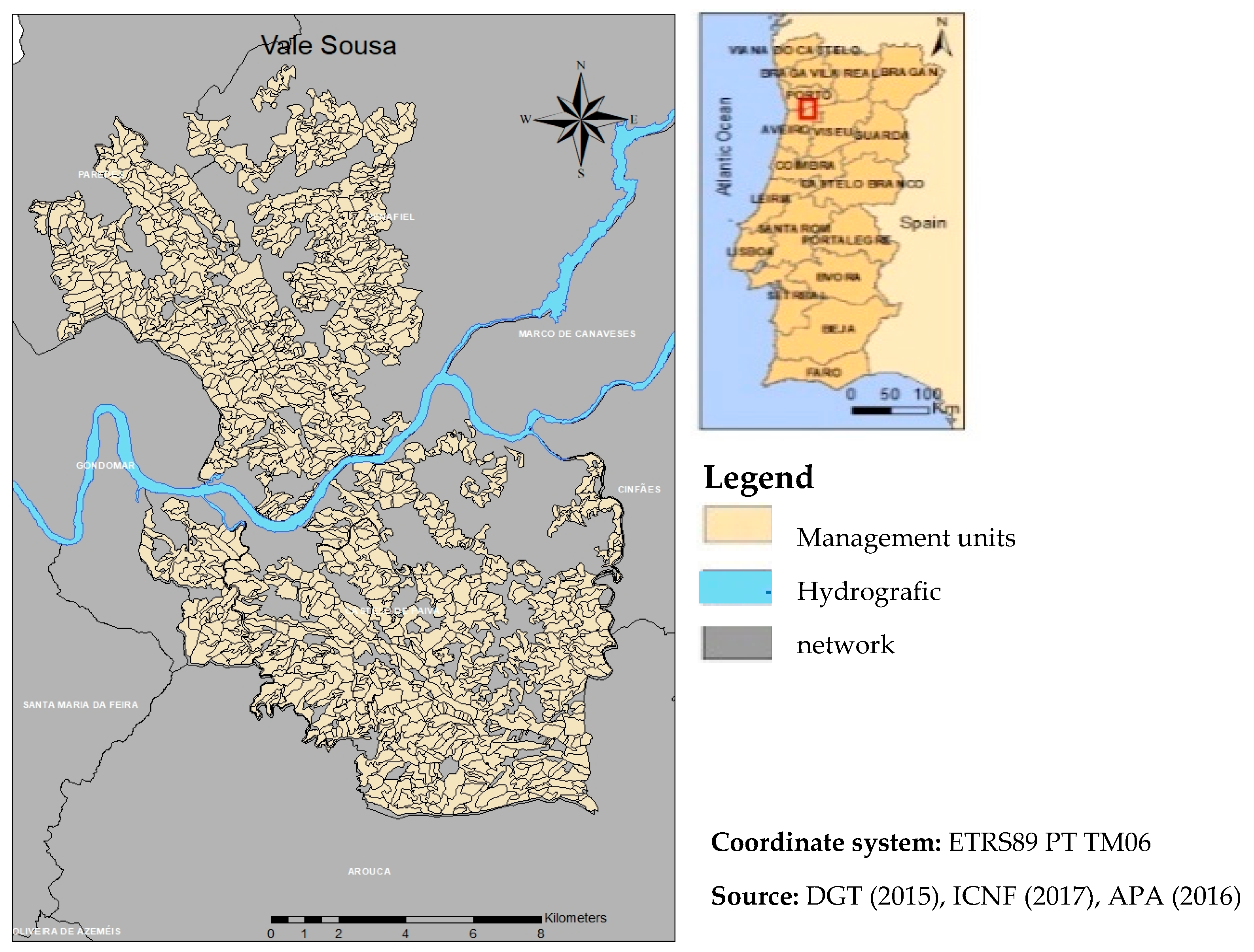
2.1. Study Area and Materials

We considered a forested landscape located in Northwest Portugal, the Joint Management Forest Areas of Entre Douro e Sousa e Castelo de Paiva (EDSCP) case study area extending over 14,779 ha and classified into 1346 stands distributed over 376 forest holdings. Current forest cover types include mixed stands composed of eucalyptus (Eucalyptus globulus L.) (dominant) with presence of maritime pine (Pinus pinaster A.), mixed stands composed of maritime pine (dominant) with presence of eucalyptus, pure chestnut (Castanea sativa M.) stands and pure even-aged eucalyptus stands.
As recent wildfires burned about 46% of the area, there is an opportunity to consider alternative cover types to determine the potential of the area to provide a wide range of ecosystem services. The introduction of these new cover types may occur in barelands, shrublands and a restoration option of recently burned stands. There is also opportunity to reconvert the existing species. In this research, we considered as alternative land uses: pure even-aged maritime pine stands, pure pedunculate oak (Quercus robur L.) stands, pure cork oak (Quercus suber L.) stands and riparian buffers along water stream systems.
The EDSCP problem thus meets the requirements to test our approach as (i) it involves a large area with a large number of stands, (ii) it provides a wide range of ecosystem services (ES) and (iii) there is a large number of forest management options for each stand. Our case study area is distributed over three counties: Castelo de Paiva (further denominated by Paiva), Paredes and Penafiel (Figure 1, Table 1). Paiva County was divided into two subareas (north and south) in order to reduce the size of management problem.

2.2. Growth and Yield Modeling and Simulation

The wSADfLOR decision support toolbox [22] was used to simulate the stand-level prescriptions (Table 2) over a planning horizon extending over 90 years. Three-year planning periods were considered. In this research, we also computed several ecosystem services provided by the forested landscape (Table 3). The computations resulted in approximately 250,100 prescriptions at stand-level along the planning horizon.

2.3. The MOIP Formulation

The model used in this study is an improved version of the linear programming model presented in [15]. Let N be the number of stands and I = {1,2,…,N} be the complete set of stand identifiers. We consider T planning periods (3 years each) in a 90-year planning horizon, i.e., in our case, T = 30. Let us also denote by M i the number of prescriptions for stand i (they include the 5 shrub cleaning options and the option to resin, or not, pure stands of maritime pine). The constraints of the problem can be formulated as follows:
j = 1 M i x i j = 1 ,           i I
i I j = 1 M i a i j t r x i j = y t r ,         t = 1 , 2 , , T ;      r R
where: x i j are the binary decision variables (1 if prescription j is applied in management unit i, or 0 otherwise); y t r stand for the provision of ecosystem services such as wood flow (harvested and thinned) for different tree species (eucalyptus, pine, chestnut, oak and cork oak), cork flow, carbon stock, fire resistance, volume of ending inventory, biodiversity, erosion and cultural services in period t; r is the index that identifies each ecosystem service; R is the full set of ecosystem services; a i j t r are the coefficients associated with ecosystem service r in prescription j applied in management unit i in each planning period t.
One of the ecosystem services y t r (let us denote it as TWOODt for convenience) is the sum of wood flows of all species in period t. To reduce wood flow fluctuation, the following constraints were added:
T W O O D t + 1 T W O O D t + δ ,       t = 1 , 2 , T 1 T W O O D t + 1 T W O O D t δ ,       t = 1 , 2 , T 1
where δ is the maximum wood flow fluctuation in m3 between consecutive periods;
and:
β r t = 1 T y t r = z r        r R
where: z r stands for the provision of ecosystem service r over the planning horizon T; the coefficients β r are equal to 1 for total values or 1/T for average values; and R ,   R R is the subset of the ecosystem services used in the tradeoff analysis.
The list of total (or average) values for ecosystem services z r includes:
  • TWOOD—total amount of wood flows;
  • CARB—average carbon stock;
  • CORK—total adult cork yield;
  • EROS—total erosion;
  • BIOD—biodiversity indicator;
  • FRES—fire resistance indicator.
These ecosystem services were used as criteria in the multi-objective optimization problem formulation. The decision maker will be interested in maximizing five criteria and minimizing two criteria:
TWOOD → max, CARB → max, CORK → max, BIOD → max, FRES → max
δ → min, EROS → min
In some cases, the restrictions:
TWOOD T W O O D _ ;   CARB C A R B _ ;   C O R K C O R K _ ;   BIOD B I O D _ ; FRES F R E S _ δ δ ¯ ,   E R O S E R O S ¯
can be imposed to cut off undesirable criteria values.
Let x be the vector of binary variables x i j ;  z the vector composed by the criteria TWOOD, CARB, CORK, BIOD, FRES, EROS, δ; X the feasible set of decision variables x defined by constraints (Equations (1)–(5)) in the decision space. Then, the problem can be represented in the standard MOIP formulation.
Maximize   or   minimize   z = f ( x )   subject   to   x X
To see the full mathematical model formulation, the reader is referred to Appendix A.

2.4. Solving the MOIP

The information about tradeoffs between management planning criteria should be provided to the decision maker in a meaningful way, meeting simplicity and user-friendliness criteria [17,18]. The methodology that we used to solve the formulated MOIP is based on the ideas proposed in [43]. It involves the approximation of the Pareto frontier in the criterion space, the visual analysis of the constructed set in the form of interactive decision maps, the choice of a preferable point z ^ (with coordinates z ^ r ) in the criterion space of z (with coordinates zr) and, finally, the solution of the model using the reference point method (RPM) proposed in [44]:
m i n i m i z e   { m a x r R   ( z ^ r z r ) + r R ε r ( z ^ r z r ) }
Subject   to   z = f ( x ) ,    x X
where ε r   are small positive parameters (to avoid weak Pareto points).
Since z ^ r is close to the non-dominated frontier of the EPH, the solution of this optimization problem is an efficient decision x * that provides the achievement vector z * that best reflects the decision-maker preferences z ^ . The RPM can be considered as a variant of the goal programming method [45,46], which is one of the most commonly used multi-objective programming methods [47] that was successfully applied [48].
In MOIP problems, attainable sets in the objective space are not continuous. They consist of discrete points corresponding to the potentially large but finite number of feasible solutions. A typical Pareto frontier for MOIP problems is represented in Figure 2, where a, b, c, d and e are non-dominated (Pareto) points. The union of their dominant cones forms the Edgeworth–Pareto hull. The EPH border is shown by the blue line a-b-c-d-e. The dominant points of the EPH and of the MOIP problem are the same. As it is easy to see in Figure 2, the EPH is not a convex set. As a consequence, some dominant, or supported [49], points can be found by maximizing linear support functions (points a, c, d and e), while others (point b) cannot be found (not supported). The exact description of the Pareto frontier of MOIP problem consists of a large number of non-dominated points, and its finding is a very difficult computational problem, especially in the case of several criteria. To describe a convex hull, it is sufficient to find its vertices.
In our approach, the Pareto frontier is used to support the selection of points using the RPM. Therefore, high accuracy is not required, and we can use the non-dominated frontier of the envelope (convex hull) of EPH (depicted by the black line in Figure 2) as a surrogate representation of the Pareto frontier of MOIP problem. Exploring the effective frontier of the feasible criterion set envelope by the IDM technique and identifying the goals on it is known as reasonable goal method [48].
To determine the validity of replacing the EPH by its convex hull, we used the following procedure: on the Pareto frontier of the envelope of the EPH constructed for a pair of criteria, a set of uniformly distributed points z ^ s , s = 1,…,S is selected for each of solution z s * defined in the set of Equation (7) (Figure 3). The distance z ^ s z s * shows the proximity of the vector z s * to the MOIP solution x s * with respect to the reference point z ^ s . Then if the value m a x s = 1 , , S z ^ s z s * is sufficiently small, we can consider the use of the envelope of EPH as acceptable for the aims of the study. A similar check can be performed in the case of three or more criteria. The envelope of EPH will be called a convex Edgeworth–Pareto hull (cEPH).

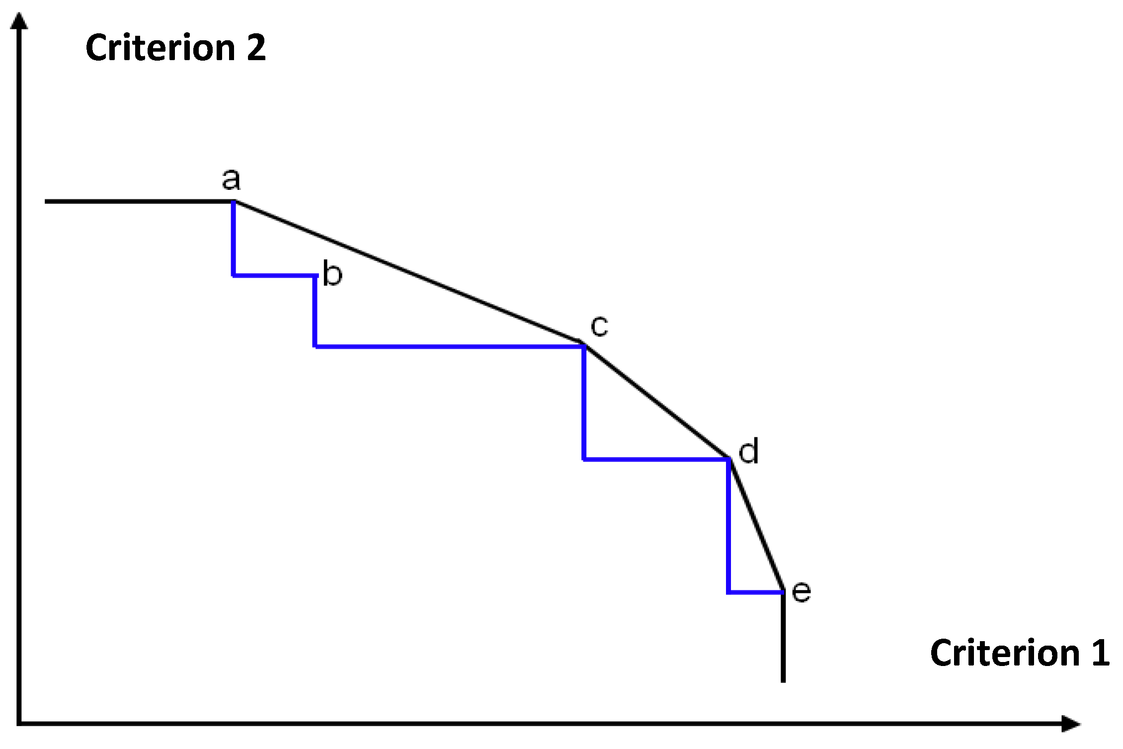
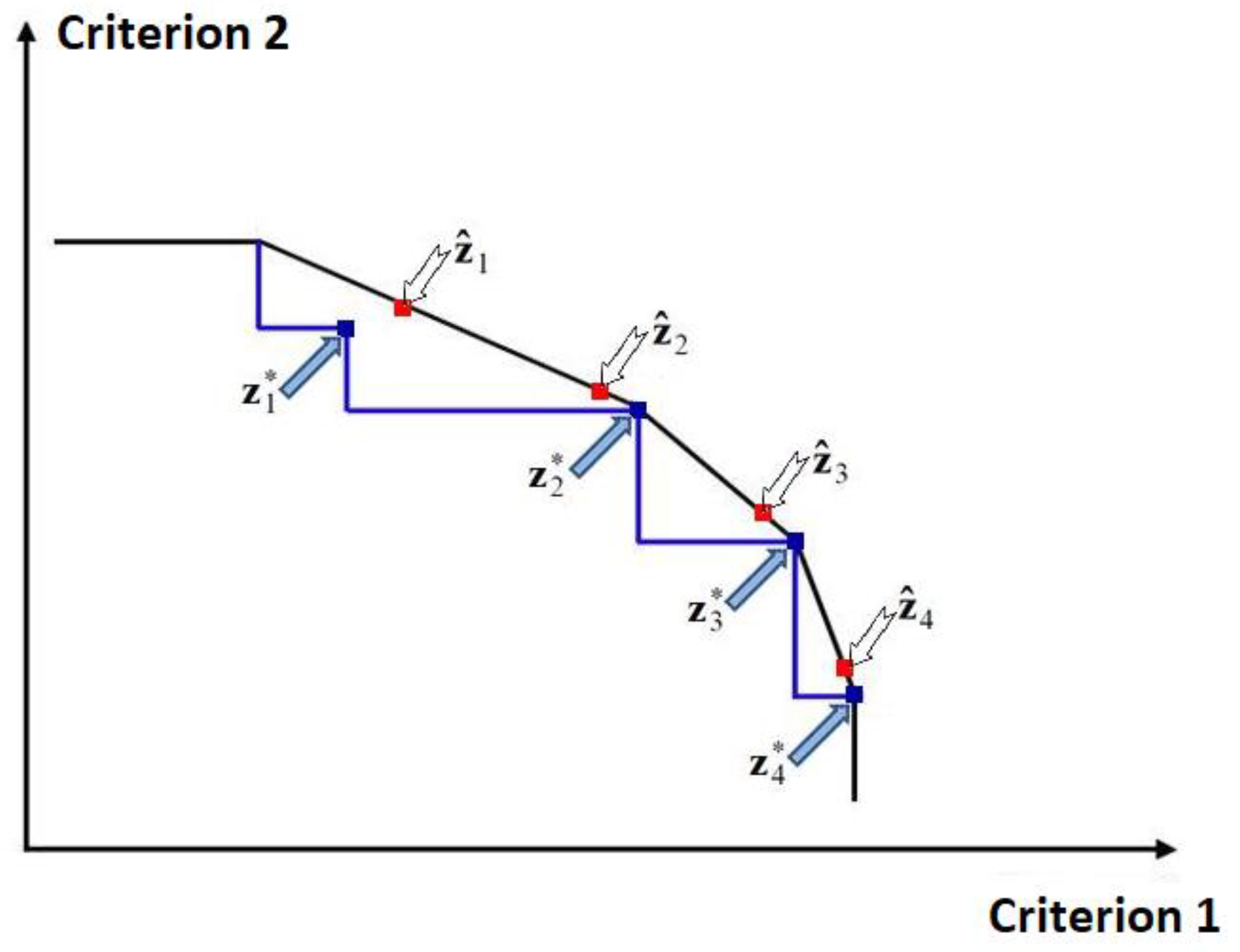
2.5. Decomposition Approach to Constructing Pareto Frontier with MOIP Problems

The problem under consideration has a large number of integer variables and constraints, which makes it difficult or even impossible to solve on modern personal computers. In addition, the construction of the Pareto frontier description requires solving a series of optimization problems. For this reason, the following decomposition approach was applied:
Suppose the initial problem is formulated as:
Maximize / minimize   z
subject   to
z = f ( x )
x X
Let the whole set I of the stand identifiers be partitioned into K non-intersecting subsets I k ,   I = I 1 I 2 I k . Forest stands belonging to the subset I k form subarea K. For each of the subareas, it is possible to introduce its own criteria vector z k and to consider the corresponding sub-problem:
Maximize / minimize   z
subject   to
z k = f ( x k )
x k X k
Then, vector z for the whole area can be found as:
z = k = 1 K z k
Taking into account that, for the problem under consideration, the Pareto frontier can be approximated by effective points of the cEPH, we can apply the approach described in [21]. Let us construct a description of cEPH for each subarea k in the form of a system of linear inequalities:
C k z k d k
where C k   is a real number matrix and d k   is real number vector, using the algorithms described in [20]. Then, we can consider the system:
Maximize / minimize   z
subject   to
z = k = 1 K z k
C k z k d k ,       k = 1 , ,   K
and construct its cEPH. Using the results of Lotov in [20], it is possible to show that the Pareto frontier of the problems (9) and (11) is the same. Due to the small size of system (11), the construction of its Pareto frontier is very easy, the computational details can be found in [21].
Now, using the IDM techniques, a certain reference point z ^ can be specified which is decomposed into z ^ 1 ,   ,   z ^ k by the RPM method applied to the system (11). In the last step, the optimal solutions of x k can be found by applying the same method for the systems (10) with reference points z ^ k .

3. Results

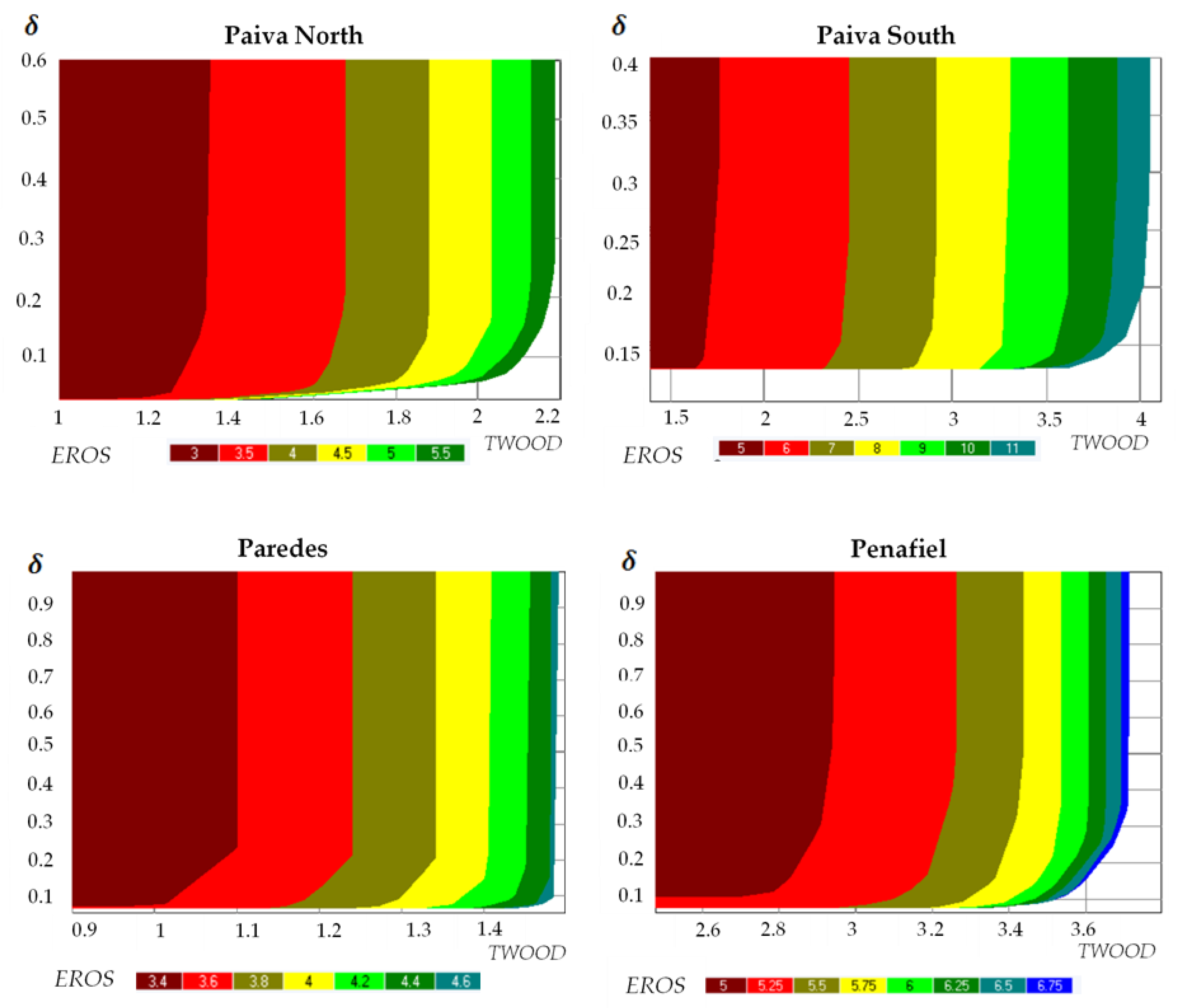
3.1. Tradeoff Analysis for the Sub-Problems

The decision maps built from each subarea were generated and analyzed using the four MOIP models. We had three objectives: maximize TWOOD, minimize EROS and minimize δ (Figure 4).

3.2. Tradeoff Analysis for the Master Problem after Merging the tradeoffs from All Subareas

The construction of the model for the forested landscape of EDSCP was obtained from the four MOIP formulations for each subarea. Since the Pareto frontier generated using MOIP formulations is convex, the feasible criteria (WOODk, EROSk and δ k) for all subareas and the corresponding polyhedral sets can be described by the system of linear inequalities. In this application, a total of 397 inequations was used to approximate the Pareto frontier of the problem for the whole EDSCP.
The generation of the Pareto frontier for the whole area is possible (Figure 5) and presents the decision maps obtained for the three criteria: maximization of TWOOD and minimization of soil erosion (EROS) and of δ as the total wood flow fluctuation in each planning period. These three criteria range between 0 and 11.5 × 10⁶ m3, 16 and 29 Mg and 0.07 and 0.39, respectively. The execution time for this problem took about 45 s to generate the Pareto frontier for the EDSCP with 250,100 prescriptions simulated in about 14,800 ha and less than one second to obtain the silvicultural plan after the selection of the desired criteria level (Table 4).
When the decision maker selects a target level of each criterion (Table 4) in the Pareto frontier (Figure 5) for the whole EDSCP, the solution retrieved provides information about the contribution of each subarea for the level of each criterion in the global problem (Table 4). Regarding the target established for total wood provision for the case-study area in the 90-year planning horizon, the subareas of Paiva South and Penafiel contribute with about 68% of the demand. Paredes County is the subarea where the wood is thinned and harvest (14% of the total) is smaller due to the smaller area. The largest values of soil erosion occur in Paiva South and in Penafiel, whereas the smallest level of erosion is accounted in Paiva North. The minimum timber flow fluctuation is about 0.05 × 10⁶ m3 in Paiva North and the maximum fluctuation is 0.17× 10⁶ m3 in Paiva South.
The approximate targets of the three criteria in each subarea were identified in the respective Pareto frontier, and the management plan was retrieved as well as the value of all criteria (Table 4).

3.3. Surrogate Pareto Frontier Accuracy

In order to validate the proposed approach to generate the convex hull of the Pareto frontier of MOIP models with binary variables, we considered two stopping criteria: precision = 0.01 and maximum number of vertices = 100. Using the Penafiel model and optimizing the TWOOD and CORK criteria, the convex Pareto hull was obtained. We tested the approach with more than 60 points to determine the precision and accuracy of the surrogate Pareto frontier. The computations were performed on a personal computer with an Intel® Core™ i7-8700 processor with a 3.20 GHz frequency and 16 Gb memory.
For demonstration, six random points with different levels of achievement of two criteria were identified in the convex Pareto hull represented by the white arrows (Figure 6), and the nearest corresponding point in the real Pareto frontier was obtained, indicated by the blue arrows (Table 5).
Our approach evidences a high accuracy since the discrepancy between the point in the Pareto hull and the nearest integer-feasible solution in the Pareto frontier is very low. The observed values have residual differences (less than 0.1%). The highest differences between the points are recorded when the point selection occurs near the extremes (horizontal and vertical edges) of the Pareto hull.
The decision maps for the three criteria were generated for each MOIP model (Figure 7), and models Paiva North and Paredes were selected due to the problem size difference. Ten random points were selected in the Pareto frontier to determine the proximity between the frontier and the real solutions (points). The results show that the discrepancy between the Pareto frontiers generated by the convexification of the supported points and the integer-feasible solution is very low (Table 6) since the highest difference between the two points (surrogate frontier and feasible point) is about 0.015% registered in point 9 in the EROS criterion in problem Paiva North. In the IDM generated for the smaller problem, Paredes, the greatest difference is about 0.003%, registered in point 7, criterion FRES.
The generation and visualization of the Pareto frontier was tested with the MOIP models for the four subareas (Paiva North, Paiva South, Paredes and Penafiel). Three combinations of two and three criteria were randomly selected and used to generate the Pareto frontiers. The average time (in seconds) to obtain the IDM for these MOIP formulations was recorded (Table 7). The problem with fewer decision variables (Table 1), Paredes, was the fastest to solve: in less than one minute when selecting two criteria and approximately 7.5 min when addressing three criteria. Problems approximately 3.5 times larger, such as Paiva North and Paiva South, took on average 75 min to be solved when considering the optimization of three criteria, whereas the Penafiel problem, with the greatest number of decision variables, generated the Pareto frontier in about 104 min.

3.4. Spatialization of the Solution in Each Block or for All Area

The plan associated with the solution for Paiva County using Paiva North and Paiva South in periods 1 and 14, as an example, (Figure 8) was visualized geographically using a new submodule associated with the Pareto frontier method. This submodule reads the criteria values in the cplex solution file and displays the corresponding harvest plan in each period of the planning horizon. In this version, the user can visualize, in each planning period, the main silvicultural options such as harvests, thinnings and cork extractions. The different colors in the map represent the species associated with the management options.
The wood flow (harvested and thinned) and cork extracted in Paiva subareas (North and South) associated with the solution and the corresponding harvest schedule are displayed in a graphical format (Figure 9). The contrast between harvest levels over the planning horizon is evident in the case of Paiva. The same happened in the case of the other problems—Paredes and Penafiel.
The user is also allowed to define the maximum limit to be harvested for each species (Equation (5)). With this limit we avoid the chart peaks on the harvested volume, leading to a new harvest plan and a new distribution of the species in the case-study area.

4. Discussion and Conclusions

This paper presents an approach for the generation and visualization of Pareto frontiers when dealing with complex problems with a large number of variables using MOIP. The method was tested with a forested case study composed of 1346 stands located in Northwestern Portugal chosen by its representability of the ownership structure as well its representativeness of forest management practices involving several species. The data and information management processes to generate the tradeoffs between the forest management decision criteria were fully automated thus meeting the forest management process efficiency requirement.
MOMP may be classified into three classes according to the phase in which the decision maker is involved in the decision-making process: the a priori methods, the interactive methods and the a posteriori or generation methods [50]. References [12,17,21,51] developed work using a posteriori methods in participatory forest planning. Given that usually there is no unique optimal solution (maximizing simultaneously all the objectives), the aim is to find the most preferred among the Pareto optimal solutions [6].
Building the Pareto frontier of multi-objective integer or mixed-integer programming problems is complicated by the non-connectedness of integer solutions and the resulting non-convexness. This topic is largely discussed in the literature, leading to the development of several approaches, such as: ε-constraint methodology (e.g., in [2,4,52,53,54]), the alpha–delta method [5] and ε-tabu constraint methodology [55]. These approaches are very effective when the problem has a small number of decision variables and of criteria to be optimized (up to two or three). Study [56] proposed the algorithm to address disconnected feasible domains that are characteristic of integer and mixed-integer programming problems. The approach proposed to approximate the convex hull was shown to be accurate, since the discrepancy between the points selected in the Pareto frontier and the real solution is small (less than 1%) and the execution times are acceptable, considering the problem size and complexity.
The large number of decision variables (for EDSCP) and complex integer programs elevate the computational cost. Thus the implementation of a decomposition approach [21] is influential to solve linear, mixed and integer programming models of large-scale forest management planning problems. Study [20] used the same technique to decompose a problem of approximating the Edgeworth–Pareto hull in a multicriteria optimization problem. The reconstruction of the master problem was possible since the EPHs for the subareas are convex and, for this reason, can be approximated by polyhedral sets with any required accuracy [43]. Other decomposition techniques have been used to address large-scale forest management problems [57,58]. Nevertheless, our technique is unique for its application to generate Pareto frontiers.
The IDM technique used in our work was simplified by the decomposition in four subareas. Users will be able to check information about landscape-wide combinations of these alternatives when making decisions, with the help of the solution visualization module that displays the management plan on a map. This is an innovation from Marques et al. [21], where the user could only check when to harvest a stand. As in [18], results also demonstrate the potential of our Pareto frontier approach to overcome the need by other methods for specifying a priori ecosystem service target levels [59,60,61]. The approach may further facilitate the estimation of the regional potential for the supply of ecosystem services and complement multiple-criteria approaches designed for that purpose (e.g., in [62]).
Further interaction with stakeholders in participatory forest planning is crucial to ensure the understanding and the further implementation of the solutions. The model formulation included timber and cork production, erosion control, carbon sequestration, cultural services, biodiversity and fire resistance. The pairwise combinations are not always conflicting, and some objectives could be derived from a reduced pool of management objectives.
This paper presents an approach for model building to increase the efficiency to solve complex problems with a large number of variables and using multi-objective mixed-integer programming. The results show the effectiveness of the approach to address obstacles such as a large number of decision variables. This research may also contribute to enhancing the analysis of tradeoffs between ecosystem services in large-scale problems and help forest managers address effectively the demand for forest products while sustaining the provision of services avoiding the fragmentation of the landscape guaranteed by the integer solutions.

Author Contributions

Conceptualization: S.M. and V.B.; methodology: S.M. and V.B.; software: V.B. and A.L.; validation; S.M., J.G.B. and V.B.; formal analysis: S.M., J.G.B. and V.B.; investigation: S.M. and V.B.; data curation: S.M. and J.G.B.; writing—original draft preparation: S.M., V.B. and J.G.B.; writing—review and editing: S.M., V.B. and J.G.B.; project administration: S.M. and J.G.B.; funding acquisition: S.M. and J.G.B. All authors have read and agreed to the published version of the manuscript.

Funding

This research was funded by national funds through the FCT—Fundação para a Ciência e a Tecnologia, I.P. in the scope of Norma Transitória—DL57/2016/CP1382/CT15. This research has also received funding from the project MODFIRE—A multiple criteria approach to integrate wildfire behavior in forest management planning with the reference PCIF/MOS/0217/2017.

Data Availability Statement

Data is already in published manuscripts or can be obtained on request.

Acknowledgments

The authors would like to thank the projects: BIOECOSYS—Forest ecosystem management decision-making methods—an integrated bio-economic approach to sustainability with the reference PTDC/ASP-SIL/30391/2017 funded by the FCT and NOBEL (Novel business models and mechanisms for the sustainable supply of and payment for forest ecosystem services) which is part of the ERA-NET Cofund ForestValue. ForestValue is a project of the EU’s Horizon 2020 Program, grant agreement No. 773324. The authors would like to thank the FCT for funding through the project CIMA, grant UIDB/04674/2020, and the Forest Research Center Project UIDB/00239/2020.

Conflicts of Interest

The authors declare no conflict of interest.

Appendix A

The MOIP formulation
Let I = {1,2,…,M} be the complete set of stand identifiers. Let us denote by I k some subset of forest stands, I K I , by T—the number of planning periods (t = 1,2,…, 30) and by N i —the number of prescriptions for each stand i (they include the five shrub cleaning options and the option to resin, or not, pure stands of maritime pine). In short, the MOIP problem formulation for this subarea may be described as follows:
i I k j = 1 N i x i j = 1 i = 1 M (A1)
i I k j = 1 N i p i n e i j t x i j = P i n e W t k   t = 1 T (A2)
i I k j = 1 N i e u c a l i p t i j t x i j = E u c W t k   t = 1 T (A3)
i I k j = 1 N i c h e s t n u t i j t x i j = C h e s t W t k   t = 1 T (A4)
i I k j = 1 N i p e n d o a k i j t x i j = P O a k W t k   t = 1 T (A5)
i I k j = 1 N i c o a k i j t x i j = C O a k W t k   t = 1 T (A6)
i I k j = 1 N i c o r k i j t x i j = C o r k t k   t = 1 T (A7)
P i n e W t k + E u c W t k + C h e s t W t k + P O o a k W t k + C o a k W t k = T w o o d t k (A8)
i I k j = 1 N i v e i i j t x i j = V E I t k   t = 1 T (A9)
i I k j = 1 N i c a r b i j t x i j = C a r b t k   t = 1 T (A10)
1 F A   i I k j = 1 N i a i f r a i t i j t x i j = F R A t k   t = 1 T (A11)
1 F A   i I k j = 1 N i a i b i o d i j t x i j = B i o d t k   t = 1 T (A12)
1 F A i I k j = 1 N i a i r a f l i n d i j t x i j = R A F L t k   t = 1 T (A13)
i I k j = 1 N i e r o s i o n i j t x i j = E r o s i o n t k   t = 1 T (A14)
i I k j = 1 N i a i x i j = A _ C T t k   f F      f = 1 8 (A15)
1 T P i n e W t k = P i n e S a w l o g s k (A16)
1 T E u c W t k = E u c P u l p W o o d k (A17)
1 T C h e s t t k = C h e s t S a w l o g s k (A18)
1 T P O a k W t k = P O a k S a w l o g s k (A19)
1 T C O a k W t k = C O a k S a w l o g s k (A20)
P i n e S a w l o g s k + E u c P u l p W o o d k + C h e s t S a w l o g s k + P O a k S a w l o g s k + C O a k S a w l o g s k = T W O O D k (A21)
1 T C o r k t t k = C O R K k (A22)
1 T 1 T C a r b t k = C A R B k (A23)
1 T 1 T F R A t k = F R E S k (A24)
1 T 1 T B i o d t k = B I O D k (A25)
1 T 1 T R A L F t k = C U L T S E R V k (A26)
1 T E r o s i o n t k = E R O S k (A27)
T W O O D t + 1 k T W O O D t k + δ k ,       t = 1 , 2 , T 1 (A28)
T W O O D t + 1 k T W O O D t k δ k ,       t = 1 , 2 , T 1 (A29)
where:
  • x i j   = 1 if prescription j is applied in management unit i, or 0 otherwise;
  • T = the number of planning periods (t = 1…30);
  • F = the number of forest management models (8);
  • C T f = the set of prescriptions that were classified as belonging to a cover type;
  • F A = total forested area in each subarea;
  • a i = the area occupied by each species in the management unit i;
  • p i n e i j t = the pine timber flow in period t that results from assigning prescription j to stand i;
  • e u c a l i p t i j t = the eucalyptus timber flow in period t that results from assigning prescription j to stand i;
  • c h e s t n u t i j t = the chestnut timber flow in period t that results from assigning prescription j to stand i;
  • p e n d o a k i j t = the pedunculated oak timber flow in period t that results from assigning to stand i the prescription j;
  • c o a k i j t = the cork oak flow in period t that results from assigning to stand i the prescription j;
  • c o r k i j t = the cork timber flow that results from assigning prescription j to stand i in period t;
  • v e i i j t = the standing volume (in m3) in the ending inventory in stand i when assigning prescription j in t;
  • c a r b i j t = average yearly carbon stock (Mg ha−1) in period t that results from assigning prescription j to stand i;
  • f r a i t i j t = fire resistance indicator in period t that results from assigning to stand i prescription j, ranging from 1 (less resistance) to 5 (highest resistance);
  • b i o d i j t = biodiversity indicator in period t that results from assigning to stand i prescription j, ranging from 0 (bare land or no biodiversity) to 8 (highest level of biodiversity);
  • r a f l i n d i j t = RAFL index or cultural services indicator in period t that results from assigning to stand i prescription j, ranging from 1 (low cultural interest) to 5 (highest cultural and recreation interest);
  • e r o s i o n i j t = the soil erosion in Mg in period t that results from assigning to stand i the prescription j;
  • A _ C T = the area assigned to cover type f;
The description of the models is as follows:
  • Equation (A1) states that only one prescription is assigned to each stand in the MOIP model.
  • Equations (A2)–(A6) define, respectively, the pine, eucalypt, chestnut, pedunculated oak and cork oak timber yield.
  • Equation (A7) defines the adult cork yield in each planning period.
  • Equation (A8) defines the total amount of wood thinned and harvested in each period.
  • Equation (A9) was included to define the standing volume in the case study area at the end of the planning horizon.
  • Equation (A10) defines the average carbon stock in the study area in each planning period.
  • Equations (A11) to (A14) define, respectively, the fire resistance indicator, biodiversity indicator, cultural services indicators and soil erosion.
  • Equations (A15) defines the area assigned to each cover type.
  • Equations (A16) to (A27) represent, respectively, the total pine sawlog yield, total eucalyptus pulpwood yield, total chestnut sawlog yield, total pedunculate oak sawlog yield, total cork oak sawlog yield, total adult cork yield, average over the 30 planning periods of carbon stock, fire resistance indicator, biodiversity indicator, cultural services indicator and total erosion across the planning horizon. These equations thus define the values of the criteria considered for testing purposes in each subarea.
  • Equations (A28) and (A29) establish a maximum fluctuation of δ between periods in the amount of wood thinned and harvested.

References

  1. Baskent, E.Z.; Keleş, S. Spatial forest planning: A review. Ecol. Model. 2005, 188, 145–173. [Google Scholar] [CrossRef]
  2. Tóth, S.F.; McDill, M.E.; Rebain, S. Finding the efficient frontier of a bi-criteria, spatially explicit, harvest scheduling problem. Forest Sci. 2006, 52, 93–107. [Google Scholar] [CrossRef]
  3. Rönnqvist, M.; D’Amours, S.; Weintraub, A.; Jofre, A.; Gunn, E.; Haight, R.G.; Martell, D.; Murray, A.; Romero, C. Operations Research challenges in forestry: 33 open problems. Ann. Oper. Res. 2015, 232, 1–30. [Google Scholar] [CrossRef]
  4. Weintraub, A.; Murray, A.T. Review of combinatorial problems induced by spatial forest harvesting planning. Discret. Appl. Math. 2006, 154, 867–879. [Google Scholar] [CrossRef]
  5. Tóth, S.F.; McDill, M.E. Finding efficient harvest schedules under three conflicting objectives. Forest Sci. 2009, 55, 117–131. [Google Scholar] [CrossRef]
  6. Mavrotas, G.; Florios, K. An improved version of the augmented ε-constraint method (AUGMECON2) for finding the exact pareto set in multi-objective integer programming problems. Appl. Math. Comput. 2013, 219, 9652–9669. [Google Scholar] [CrossRef]
  7. Benson, H.P. Multi-Objective Optimization: Pareto Optimal Solutions, Properties. In Encyclopedia of Optimization; Floudas, C.A., Pardalos, P.M., Eds.; Springer: Boston, MA, USA, 2001. [Google Scholar]
  8. Branke, J.; Deb, K.; Miettinen, K.; Slowinski, R.; Miettinen, K. Preface. In Multiobjective Optimization; Branke, J., Ed.; Springer: Berlin/Heidelberg, Germany, 2008; pp. V–XII. [Google Scholar]
  9. Miettinen, K. A Posteriori Methods. In Nonlinear Multiobjective Optimization. International Series in Operations Research & Management Science; Springer: Boston, MA, USA, 1998; Volume 12. [Google Scholar]
  10. Miettinen, K. Nonlinear Multiobjective Optimization; Kluwer Academic Publishers: Boston, MA, USA, 1999. [Google Scholar]
  11. Lotov, A.; Miettinen, K. Visualizing the Pareto Frontier. In Computer Vision; Branke, J., Ed.; Springer: Berlin/Heidelberg, Germany, 2008; pp. 213–243. [Google Scholar]
  12. Marques, S.; Marto, M.; Bushenkov, V.; McDill, M.; Borges, J. Addressing Wildfire Risk in Forest Management Planning with Multiple Criteria Decision Making Methods. Sustainability 2017, 9, 298. [Google Scholar] [CrossRef] [Green Version]
  13. Trautmann, H.; Mehnen, J. Preference-based Pareto optimization in certain and noisy environments. Eng. Optim. 2009, 41, 23–38. [Google Scholar] [CrossRef]
  14. Miettinen, K. Introduction to Multiobjective Optimization: Noninteractive Approaches. In Multiobjective Optimization; Branke, J., Ed.; Springer: Berlin/Heidelberg, Germany, 2008; pp. 1–26. [Google Scholar]
  15. Geoffrion, A.M. Proper efficiency and the theory of vector maximization. J. Math. Anal. Appl. 1968, 22, 618–630. [Google Scholar] [CrossRef] [Green Version]
  16. Eswaran, P.K.; Ravindran, A.; Moskowitz, H. Algorithms for nonlinear integer brcriterion problems. J. Optim. Theory Appl. 1989, 63, 261–279. [Google Scholar] [CrossRef]
  17. Borges, J.G.; Garcia-Gonzalo, J.; Bushenkov, V.; McDill, M.E.; Marques, S.; Oliveira, M. Addressing Multicriteria Forest Management with Pareto Frontier Methods: An Application in Portugal. For. Sci. 2014, 60, 63–72. [Google Scholar] [CrossRef] [Green Version]
  18. Borges, J.G.; Marques, S.; Garcia-Gonzalo, J.; Rahman, A.U.; Bushenkov, V.; Sottomayor, M.; Carvalho, P.O.; Nordström, E.-M. A Multiple Criteria Approach for Negotiating Ecosystem Services Supply Targets and Forest Owners’ Programs. For. Sci. 2017, 63, 49–61. [Google Scholar] [CrossRef]
  19. Marto, M.; Reynolds, K.M.; Borges, J.G.; Bushenkov, V.A.; Marques, S. Combining Decision Support Approaches for Optimizing the Selection of Bundles of Ecosystem Services. Forests 2018, 9, 438. [Google Scholar] [CrossRef] [Green Version]
  20. Lotov, A.V. Decomposition methods for the Edgeworth-Pareto hull approximation. Comput. Math. Math. Phys. 2015, 55, 1653–1664. [Google Scholar] [CrossRef]
  21. Marques, S.; Bushenkov, V.A.; Lotov, A.V.; Marto, M.; Borges, J.G. Bi-Level Participatory Forest Management Planning Supported by Pareto Frontier Visualization. For. Sci. 2019, 66, 490–500. [Google Scholar] [CrossRef]
  22. Marto, M.; Reynolds, K.M.; Borges, J.G.; Bushenkov, V.A.; Marques, S.; Marques, M.; Barreiro, S.; Botequim, B.; Tomé, M. Web-Based Forest Resources Management Decision Support System. Forests 2019, 10, 1079. [Google Scholar] [CrossRef] [Green Version]
  23. Gómez-García, E.; Crecente-Campo, F.; Anta, M.B.; Diéguez-Aranda, U. A disaggregated dynamic model for predicting volume, biomass and carbon stocks in even-aged pedunculate oak stands in Galicia (NW Spain). Eur. J. For. Res. 2015, 134, 569–583. [Google Scholar] [CrossRef]
  24. Gómez-García, E.; Diéguez-Aranda, U.; Cunha, M.; Rodríguez-Soalleiro, R. Comparison of harvest-related removal of aboveground biomass, carbon and nutrients in pedunculate oak stands and in fast-growing tree stands in NW Spain. For. Ecol. Manag. 2016, 365, 119–127. [Google Scholar] [CrossRef]
  25. Almeida, A.M.; Tomé, J.; Tomé, M. Development of a system to predict the evolution of individual tree mature cork caliber over time. For. Ecol. Manag. 2010, 260, 1303–1314. [Google Scholar] [CrossRef]
  26. Paulo, J.A.; Tomé, M. Equações para Estimação do Volume e Biomassa de Duas Espécies de Carvalhos: Quercus suber e Quercus ilex; Publicações GIMREF—RC1/2006; Departamento de Engenharia Florestal, Instituto Superior de Agronomia: Lisboa, Portugal, 2006; p. 21. Available online: http://hdl.handle.net/10400.5/1730Â (accessed on 10 August 2021).
  27. Paulo, J.A.; Tomé, M. Predicting mature cork biomass with t years of growth based in one measurement taken at any other age. For. Ecol. Manag. 2010, 259, 1993–2005. [Google Scholar] [CrossRef]
  28. Paulo, J.A. Desenvolvimento de um Sistema para Apoio à Gestão Sustentável de Montados de Sobro. Ph.D. Thesis, Universidade Técnica de Lisboa, Instituto Superior de Agronomia, Lisboa, Portugal, 2011. Available online: http://hdl.handle.net/10400.5/3850 (accessed on 10 August 2021).
  29. Paulo, J.A.; Tomé, J.; Tomé, M. Nonlinear fixed and random generalized height–diameter models for Portuguese cork oak stands. Ann. For. Sci. 2011, 68, 295–309. [Google Scholar] [CrossRef] [Green Version]
  30. Paulo, J.A.; Palma, J.; Gomes, A.A.; Faias, S.P.; Tomé, J.; Tomé, M. Predicting site index from climate and soil variables for cork oak (Quercus suber L.) stands in Portugal. New For. 2015, 46, 293–307. [Google Scholar] [CrossRef] [Green Version]
  31. Tomé, J.; Tomé, M.; Barreiro, S.; Paulo, J.A. Age-independent difference equations for modelling tree and stand growth. Can. J. For. Res. 2006, 36, 1621–1630. [Google Scholar] [CrossRef]
  32. Claessens, H.; Oosterbaan, A.; Savill, P.; Rondeux, J. A review of the characteristics of black alder (Alnus glutinosa (L.) Gaertn.) and their implications for silvicultural practices. Forests 2010, 83, 163–175. [Google Scholar] [CrossRef] [Green Version]
  33. Rodríguez-González, P.M.; Stella, J.; Campelo, F.; Ferreira, M.T.; Albuquerque, A. Subsidy or stress? Tree structure and growth in wetland forests along a hydrological gradient in Southern Europe. For. Ecol. Manag. 2010, 259, 2015–2025. [Google Scholar] [CrossRef]
  34. Quercus Robur Simulator for Galicia. Available online: https://manuelar.shinyapps.io/Quercusrobur_SimGaliza/ (accessed on 14 July 2021).
  35. Barreiro, S.; Rua, J.; Tomé, M. StandsSIM-MD: A Management Driven forest SIMulator. For. Syst. 2016, 25, 7. [Google Scholar] [CrossRef] [Green Version]
  36. Ferreira, L.; Constantino, M.; Borges, J.; Garcia-Gonzalo, J. Addressing Wildfire Risk in a Landscape-Level Scheduling Model: An Application in Portugal. For. Sci. 2015, 61, 266–277. [Google Scholar] [CrossRef] [Green Version]
  37. Rodrigues, A.R.; Marques, S.; Botequim, B.; Marto, M.; Borges, J.G. Forest management for optimizing soil protection: A land-scape-level approach. For. Ecosyst. 2021, 8, 50. [Google Scholar] [CrossRef]
  38. Botequim, B.; Zubizarreta-Gerendiain, A.; Garcia-Gonzalo, J.; Silva, A.; Marques, S.; Fernandes, P.; Pereira, J.M.C.; Tomé, M.; Fernandes, P. A model of shrub biomass accumulation as a tool to support management of Portuguese forests. iForest—Biogeosci. For. 2015, 8, 114–125. [Google Scholar] [CrossRef] [Green Version]
  39. Biber, P.; Maarten, T.N.; Black, K.; Borga, M.; Borges, J.G.; Felton, A.; Hoogstra-Klein, M.; Lindbladh, M.; Zoccatelli, D. ALTERFOR WP3; Deliverable 3.2.—Synthesis Report: Discrepancies between ES Needs and ES Outputs under Current FMMs. 2018, p. 44. Available online: https://alterfor-project.eu/files/alterfor/download/Deliverables/D3.2%20Synthesis%20report.pdf (accessed on 5 July 2019).
  40. Nieuwenhuis, M.; Biber, P. Milestone 11—Projections with Current FMMs Per Case Study; University College Dublin: Dublin, Ireland; Technical University of Munich: Munich, Germany, 2018. [Google Scholar]
  41. Botequim, B.; Bugalho, M.N.; Rodrigues, A.R.; Marques, S.; Marto, M.; Borges, J.G. Combining Tree Species Composition and Understory Coverage Indicators with Optimization Techniques to Address Concerns with Landscape-Level Biodiversity. Land 2021, 10, 126. [Google Scholar] [CrossRef]
  42. Pretzsch, H. Forest dynamics, growth and yield. In Forest Dynamics; Growth and Yield; Springer: Berlin/Heidelberg, Germany, 2009; pp. 1–39. [Google Scholar]
  43. Lotov, A.V.; Bushenkov, V.A.; Kamenev, G.K. Interactive Decision Maps: Approximation and Visualization of Pareto Frontier; Kluwer Academic Publishers: Norwell, MA, USA, 2004; p. 319. [Google Scholar]
  44. Wierzbicki, A.P. A Mathematical Basis for Satisficing Decision Making. In Organizations: Multiple Agents with Multiple Criteria; Springer: Berlin/Heidelberg, Germany, 1981; pp. 465–486. [Google Scholar]
  45. Romero, C.; Tamiz, M.; Jones, D.F. Goal programming; compromise programming and reference point method formulations: Linkages and utility interpretations. J. Oper. Res. Soc. 1998, 49, 986–991. [Google Scholar] [CrossRef]
  46. Ogryczak, W. On goal programming formulations of the reference point method. J. Oper. Res. Soc. 2001, 52, 691–698. [Google Scholar] [CrossRef]
  47. Colapinto, C.; Jayaraman, R.; Marsiglio, S. Multi-criteria decision analysis with goal programming in engineering; manage-ment and social sciences: A state-of-the art review. Ann. Oper. Res. 2017, 251, 7–40. [Google Scholar] [CrossRef] [Green Version]
  48. Tamiz, M.; Mirrazavi, S.; Jones, D.F. Extensions of Pareto efficiency analysis to integer goal programming. Omega-Int. J. Manag. S 1999, 27, 179–188. [Google Scholar] [CrossRef]
  49. T’Kindt, V.; Billaut, J. Multicriteria Scheduling: Theory, Models and Algorithms; Springer: New York, NY, USA, 2002; p. 303. [Google Scholar]
  50. Hwang, C.L.; Masud, A.I. Multiple Objective Decision Making. Methods and Applications: A State of the Art Survey; Lecture Notes in Economics and Mathematical Systems 164; Springer: Berlin, Germany, 1979. [Google Scholar]
  51. Nordström, E.-M.; Eriksson, O.; Öhman, K. Integrating multiple criteria decision analysis in participatory forest planning: Experience from a case study in northern Sweden. For. Policy Econ. 2010, 12, 562–574. [Google Scholar] [CrossRef] [Green Version]
  52. Haimes, Y. On a bicriterion formulation of the problems of integrated system identification and system optimization. IEEE Trans. Syst. Man Cybern. 1971, 1, 296–297. [Google Scholar]
  53. Ehrgott, M.; Ruzika, S. Improved ε-Constraint Method for Multiobjective Programming. J. Optim. Theory Appl. 2008, 138, 375–396. [Google Scholar] [CrossRef]
  54. Zhang, W.; Reimann, M. A simple augmented ∊-constraint method for multi-objective mathematical integer programming problems. Eur. J. Oper. Res. 2014, 234, 15–24. [Google Scholar] [CrossRef]
  55. Soylu, B.; Yıldız, G.B. An exact algorithm for biobjective mixed integer linear programming problems. Comput. Oper. Res. 2016, 72, 204–213. [Google Scholar] [CrossRef]
  56. Burachik, R.S.; Kaya, C.Y.; Rizvi, M.M. Algorithms for generating Pareto fronts of multi-objective integer and mixed-integer programming problems. Eng. Optim. 2021, 1–13. [Google Scholar] [CrossRef]
  57. Guignard, M.; Kim, S. Lagrangean decomposition: A model yielding stronger lagrangean bounds. Math. Program. 1987, 39, 215–228. [Google Scholar] [CrossRef]
  58. Hoganson, H.; Rose, D. A Simulation Approach for Optimal Timber Management Scheduling. For. Sci. 1984, 30, 220–238. [Google Scholar] [CrossRef]
  59. Nordström, E.-M.; Romero, C.; Eriksson, O.; Öhman, K. Aggregation of preferences in participatory forest planning with multiple criteria: An application to the urban forest in Lycksele, Sweden. Can. J. For. Res. 2009, 39, 1979–1992. [Google Scholar] [CrossRef]
  60. Diaz-Balteiro, L.; Gonzalez-Pachon, J.; Romero, C. Forest management with multiple criteria and multiple stakeholders: An application to two public forests in Spain. Scand. J. For. Res. 2009, 24, 87–93. [Google Scholar] [CrossRef]
  61. Eyvindson, K.; Kangas, A. Evaluating the required scenario set size for stochastic programming in forest management planning: Incorporating inventory and growth model uncertainty. Can. J. For. Res. 2016, 46, 340–347. [Google Scholar] [CrossRef] [Green Version]
  62. Koschke, L.; Fürst, C.; Frank, S.; Makeschin, F. A multi-criteria approach for an integrated land-cover-based assessment of ecosystem services provision to support landscape planning. Ecol. Indic. 2012, 21, 54–66. [Google Scholar] [CrossRef]
Figure 1. Location of the case-study area showing subareas.
Forests 12 01244 g001
Figure 2. Approximation of the Pareto frontier by its convex hull (the surrogate frontier). The blue line represents the Pareto frontier for an integer variable model; the black line—convex Pareto hull for the same model.
Forests 12 01244 g002
Figure 3. Validation scheme. Red dots represent the point selected in the surrogate frontier ( z ^ s ). Blue dots are the feasible solutions ( z s * ) for MOIP.
Forests 12 01244 g003
Figure 4. Tradeoffs between three ecosystem services in each subarea. TWOOD—total amount of wood harvested and thinned (in ×106 m3), EROS—representing the total soil erosion (in ×106 Mg) and δ—representing the maximum wood flow fluctuation (in ×106 m3). Each of the 6 (Paiva North), 7 (Paiva South and Paredes) and 8 (Penafiel) decision maps corresponds to a level of soil erosion.
Forests 12 01244 g004
Figure 5. Tradeoffs between three ecosystem services in each subarea. TWOOD—total amount of wood harvested and thinned (in ×106 m3), EROS—representing the total soil erosion (in ×106 Mg) and δ—representing the wood flow fluctuation (in ×106 m3). Each of the 7 decision maps corresponds to a level of soil erosion.
Forests 12 01244 g005
Figure 6. Accuracy of the convex Edgeworth–Pareto hull (cEPH) with respect to the Pareto frontier for the Penafiel model. White arrows represent the points in the cEPH and blue arrows the location of the nearest point in the real Pareto frontier.
Forests 12 01244 g006
Figure 7. Tradeoffs between three ecosystem services in each sub area. (a) TWOOD—total amount of wood harvested and thinned (in ×106 m3), (b) EROS—representing the total soil erosion (in ×106 Mg) and δ—representing the wood flow fluctuation (in ×106 m3). Each of the 7 decision maps corre-sponds to a level of soil erosion.
Forests 12 01244 g007
Figure 8. Silvicultural intervention plan retrieved from the final solution represented in colors for the different species (e.g., dark green are stands with maritime pine that are harvested whereas light green are stands with maritime pine that will be thinned in the specific period). Where: Ct-thin—thinning of chestnut, Ct-harv—full harvest of chestnut, Ec-harv—harvest of eucalyptus, Pb-thin—thinning of maritime pine, Pb-harv—full harvest of maritime pine, Qr-thin—thinning of pedunculate oak, Qr-harv—full harvest of pedunculate oak, Sb-thin—thinning of cork oak, Sb-thco—cork extraction and thinning of cork oak, Sb-cork—cork extraction of cork oak.
Forests 12 01244 g008
Figure 9. Wood (in m3) and cork (in arrobas) flow for each species in the Paiva block. The black line represents the sum of the wood harvested in each period of all species using a δ of 0.07 × 10⁶ m3.
Forests 12 01244 g009
Table 1. Entre Douro e Sousa e Castelo de Paiva case-study area characterization.
PaivaParedesPenafielEDSCP
NorthSouth
Area (ha)293646382156506714,838
Number of stands3623521814581373
Number of. prescriptions73,90070,05020,20085,950250,100
Table 2. Prescriptions simulated for each species using growth/yield models and simulators used.
SpeciesPedunculate OakCork OakRiparian
Prescriptions-Silvicultural operationsPlantation (a)16001600-
Replanting (b)2020-
Pruning (c,d)23--
Thinning (d)27, 37, 4515, 30, 40, 58, 76-
Wilson Factor0.2--
Debarking (d,e)-30, 40, +(9)-
Final Harvest (d)40 to 60 (10)--
Type managementEven-agedEven-agedEven-aged
Growth model[23,24]SUBER
[25,26,27,28,29,30]
[31,32,33]
Simulator[34]StandSIM/MD
[35]
Yield table
Where: (a) number of plants per ha; (b) in percentage; (c) only applicable to pedunculate oak; (d) year; (e) only applicable to cork oak; in parenthesis () the interval between silvicultural operations.
Table 3. References for the modeling, simulation and computation of the integrated ecosystem services.
Ecosystem ServiceRangeReferences
Fire resistance1–5[12,36]
Soil erosion-[37]
Biodiversity0–8[38,39,40,41]
Cultural services1–5[42]
Table 4. Selection of a target level of three criteria (TWOOD, EROS and δ) in the Pareto frontier generated for the EDSCP and the contribution of each subarea. Run execution times to generate Pareto frontiers with 3 criteria and the level of all criteria in the subareas, when selecting the point corresponding to respective contribution for the final target (Figure 4).
Target Level of Each Criterion in the EDSCP ProblemContribution of Each Subarea to the Target Level of Each Criterion
Paiva NorthPaiva SouthParedesPenafiel
Optimized CriteriaTWOOD (×106 m3)9.16611.67382.75741.27473.4602
δ (×106 m3)0.11350.05600.17120.08160.1464
EROS (×106 Mg)19.81513.6524665113.78785.7238
Solution in the subareas
PF generation time (in seconds)332713594844367
Optimized CriteriaTWOOD (×106 m3)1.66572.75041.27043.4611
δ (×106 m3)0.05390.16170.08370.1375
EROS (×106 Mg)3.65826.64963.77895.7218
Other criteriaCARB (×106 Mg ha−1)2.02642.67910.36212.6061
Cork (×105 arroba)0.03160.00000.00000.0162
CULTSERV (-)0.88241.28012.93423.3211
FRES (-)2.61972.04562.08692.1123
BIOD (-)3.14012.98152.64672.7561
Area_Ct (ha)64173119
Area_Ec (ha)7261833542865
Area_Mp (ha)1315130015693824
Area_Po (ha)774143918203
Area_Rp (ha)2248238
Area_Co (ha)340018
Where: arroba = 14.7 kg.
Table 5. The level of criteria selected in the convex Edgeworth–Pareto hull for the MOIP formulation in problem of Penafiel and the nearest real point (the integer-feasible solution).
Convex Edgeworth–Pareto HullNearest Pareto Frontier Point
TWOODCORKTWOODCORK
Point 12.8001.8852.8011.885
Point 22.9961.7113.0001.711
Point 33.2001.5093.2001.523
Point 43.3991.1993.3991.201
Point 53.5980.7953.5990.802
Point 63.6690.5653.6700.570
Table 6. The level of criteria selected in the convex approximation of the Pareto frontier for the MOIP formulation for Paiva North and Paredes and the feasible point where SF: surrogate frontier and FP: nearest feasible point.
ModelCriteria Point1Point2Point3Point4Point5Point6Point7Point8Point9Point10
Paiva NorthTWOODSF1.28241.32981.52471.41541.72872.07472.12022.16762.17491.8575
FP1.28261.32991.51991.41151.72872.07472.12042.16762.17491.8561
CARBSF2.97412.57043.80644.30274.09043.78614.20183.41973.93274.9365
FP2.99592.59153.80984.30274.15633.85644.22303.51134.06484.9351
EROSSF3.00003.00003.50003.50004.00005.00005.50005.50006.00006.5000
FP2.99993.00003.50473.49993.99985.00005.48225.50005.90806.4702
ParedesTWOODSF1.41631.40211.38371.45191.29461.41201.45501.43471.36961.2811
FP1.41621.40301.38521.45201.29501.41231.45531.43471.36961.2817
FRESSF3.13453.20273.21953.21713.28293.27873.27963.27633.29303.2960
FP3.13483.20273.21973.21723.28293.27963.26933.27633.29303.2961
EROSSF5.00005.00005.00004.80004.80004.60004.60004.40004.40004.4000
FP5.00005.00015.00094.80054.80104.60084.61514.44204.40254.4193
Table 7. Average time needed (in seconds) to generate the Pareto frontier with two and three criteria in each subarea.
Model AliasPareto Frontier Generation (in Seconds)
2 Criteria3 Criteria
Paiva North2235219
Paiva South3133836
Penafiel4366255
Paredes47442
Publisher’s Note: MDPI stays neutral with regard to jurisdictional claims in published maps and institutional affiliations.

