
Price Volatility Transmission in China’s Hardwood Lumber Imports

Abstract
:1. Introduction
2. Materials and Methods
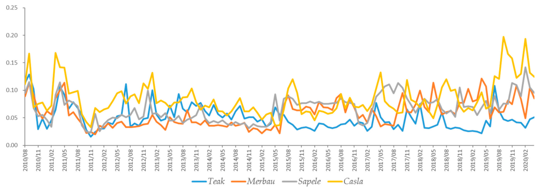
2.1. Overall Trend of Price Volatility
2.2. Methodology
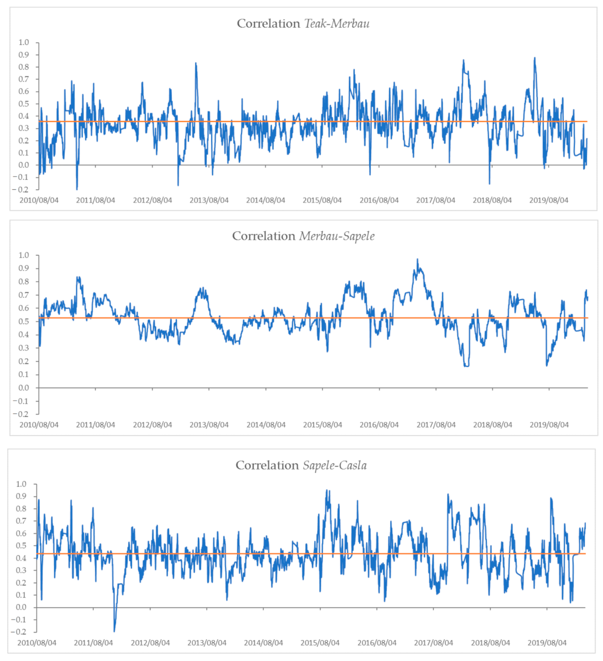
3. Results
4. Discussion
5. Conclusions
Author Contributions
Funding
Data Availability Statement
Conflicts of Interest
References
- State Forestry Administration in China. China Forestry Statistical Yearbook; Translated title into English; China Forestry Publishing House: Beijing, China, 2018. [Google Scholar]
- Liu, F.; Wheiler, K.; Ganguly, I.; Hu, M. Sustainable Timber Trade: A Study on Discrepancies in Chinese Logs and Lumber Trade Statistics. Forests 2020, 11, 205. [Google Scholar] [CrossRef] [Green Version]
- Parajuli, R.; Zhang, D.W. An Econometric Study of the Hardwood Sawtimber Stumpage Market in Louisiana. For. Prod. J. 2017, 67, 91–100. [Google Scholar] [CrossRef]
- Food and Agriculture Organization of the United Nations. Available online: http://www.fao.org/faostat/en/#data/FT (accessed on 28 October 2020).
- Yang, L.; Yin, Z.; Gan, J.; Wang, F. Asymmetric Price Transmission of Hardwood Lumber Imported by China after Imposition of the Comprehensive Commercial Logging Ban in All Natural Forests. Forests 2020, 11, 200. [Google Scholar] [CrossRef] [Green Version]
- Zhu, G. Status, problems and development suggestions of China’s wood market (Translated Title into English). For. Prod. Ind. 2003, 2, 3–7. [Google Scholar] [CrossRef]
- State Forestry Administration in China. The Report of Forestry Development in China; Translated title into English; China Forestry Publishing House: Beijing, China, 2016. [Google Scholar]
- State Forestry Administration in China. The Report of Forestry Development in China; Translated title into English; China Forestry Publishing House: Beijing, China, 2017. [Google Scholar]
- Kavussanos, M.G.; Visvikis, I.D.; Dimitrakopoulos, D.N. Economic spillovers between related derivatives markets: The case of commodity and freight markets. Transp. Res. Part E Logist. Transp. Rev. 2014, 68, 79–102. [Google Scholar] [CrossRef]
- Abdelradi, F.; Serra, T. Asymmetric price volatility transmission between food and energy markets: The case of Spain. Agric. Econ. 2015, 46, 503–513. [Google Scholar] [CrossRef]
- Apergis, N.; Rezitis, A. Agricultural price volatility spillover effects: The case of Greece. Eur. Rev. Agric. Econ. 2003, 30, 389–406. [Google Scholar] [CrossRef]
- Gardebroek, C.; Hernandez, M.A.; Robles, M. Market interdependence and volatility transmission among major crops. Agric. Econ. 2016, 47, 141–155. [Google Scholar] [CrossRef] [Green Version]
- State Forestry Administration in China. China Forestry Statistical Yearbook; Translated title into English; China Forestry Publishing House: Beijing, China, 2017. [Google Scholar]
- Mao, C.; Yan, X. Analysis of the status quo and development trend of broadleaved lumber market in China (Translated title into English). Int. Wood Ind. 2019, 49, 25–27. [Google Scholar]
- Bergmann, D.; O’Connor, D.; Thümmel, A. Price and volatility transmission in, and between, skimmed milk powder, livestock feed and oil markets. Outlook Agric. 2017, 46, 248–257. [Google Scholar] [CrossRef]
- Nazlioglu, S.; Erdem, C.; Soytas, U. Volatility spillover between oil and agricultural commodity markets. Energy Econ. 2013, 36, 658–665. [Google Scholar] [CrossRef]
- Sendhil, R.; Kar, A.; Mathur, V.C.; Jha, G.K. Price Discovery, Transmission and Volatility: Evidence from Agricultural Commodity Futures. Agric. Econ. Res. Rev. 2013, 26, 41–54. [Google Scholar]
- An, H.; Qiu, F.; Zheng, Y. How do export controls affect price transmission and volatility spillovers in the Ukrainian wheat and flour markets? Food Policy 2016, 100, 142–150. [Google Scholar] [CrossRef]
- Saghaian, S.; Nemati, M.; Walters, C.; Chen, B. Asymmetric Price Volatility Transmission between U.S. Biofuel, Corn, and Oil Markets. J. Agric. Resour. Econ. 2018, 43, 46–60. [Google Scholar]
- Ben Abdallah, M.; Fekete Farkas, M.; Lakner, Z. Analysis of meat price volatility and volatility spillovers in Finland. Agric. Econ. 2020, 66, 84–91. [Google Scholar] [CrossRef]
- Ferrer-Pérez, H.; Gracia-de-Rentería, P. Asymmetric Price Volatility Transmission in the Spanish Fresh Wild Fish Supply Chain. Mar. Resour. Econ. 2020, 35, 65–81. [Google Scholar] [CrossRef]
- Yan, S.; Kameyama, H.; Isoda, H.; Qian, J.; Shoichi, I. Effects of international grain prices on volatility of domestic grain prices in 24 developing countries. J. Fac. Agric. 2016, 61, 225–232. [Google Scholar]
- Sinha, K.; Panwar, S.; Alam, W.; Singh, K.N.; Gurung, B.; Paul, R.K.; Mukherjee, A. Price volatility spillover of Indian onion markets: A comparative study. Indian J. Agric. Sci. 2018, 88, 114–120. [Google Scholar]
- Kakhki, M.D.; Farsi, M.M.; Fakari, B.; Kojori, M. Volatility Transmission of Barley World Price to the Domestic Market of Iran and the Role of Iran Mercantile Exchange: An Application of BEKK Model. New Medit 2019, 18, 97–108. [Google Scholar] [CrossRef]
- Capitanio, F.; Rivieccio, G.; Adinolfi, F. Food Price Volatility and Asymmetries in Rural Areas of South Mediterranean Countries: A Copula-Based GARCH Model. Int. J. Environ. Res. Public Health 2020, 17, 5855. [Google Scholar] [CrossRef] [PubMed]
- Fakari, B.; Aliabadi, M.M.F.; Mahmoudi, H.; Kojori, M. Volatility spillover and price shocks in Iran’s meat market. Custos Agronegocio 2016, 12, 84–98. [Google Scholar]
- Perifanis, T.; Dagoumas, A. Price and Volatility Spillovers Between the US Crude Oil and Natural Gas Wholesale Markets. Energies 2018, 11, 2757. [Google Scholar] [CrossRef] [Green Version]
- Živkov, D.; Kuzman, B.; Subić, J. What Bayesian quantiles can tell about volatility transmission between the major agricultural futures? Agric. Econ. 2020, 66, 215–225. [Google Scholar] [CrossRef]
- Chen, Y.; Zheng, B.; Qu, F. Modeling the nexus of crude oil, new energy and rare earth in China: An asymmetric VAR-BEKK (DCC)-GARCH approach. Resour. Policy 2020, 65, 1–11. [Google Scholar] [CrossRef]
- Grushecky, S.T.; Buehlmann, U.; Schuler, A.; Luppold, W.; Cesa, E. Decline in the US furniture industry: A case study of the impacts to the hardwood lumber supply chain. Wood Fiber Sci. 2006, 38, 365–376. [Google Scholar]
- Lookose, S. Traditional teak wood articles used in households of Nilambur and Malapuram areas of Kerala. Indian J. Tradit. Know. 2008, 7, 108–111. [Google Scholar]
- Ratnasingam, J.; Liat, L.C.; Ramasamy, G.; Mohamed, S.; Senin, A.L. Attributes of sawn timber important for the manufacturers of value-added wood products in Malaysia. BioResources 2016, 11, 8297–8306. [Google Scholar] [CrossRef] [Green Version]
- Chen, X.; Guo, X.; Ran, J.; Zhu, Y.; Du, G.; Xu, Y.; Pan, B. Imported Wood Primary Color Manual; Translated title into English; Shanghai Science and Technology Publishing House: Shanghai, China, 2004; ISBN 7-532-37452-1. [Google Scholar]
- Isabelle, P.; Robert, M. Methods to Analyse Agricultural Commodity Price Volatility; Springer: New York, NY, USA, 2010; Chapter 4; pp. 45–61. ISBN 978-1-4419-7633-8. [Google Scholar]
- Aktan, B.; Korsakienė, R.; Smaliukiene, R. Time-varying volatility modelling of Baltic stock markets. J. Bus. Econ. Manag. 2010, 11, 511–532. [Google Scholar] [CrossRef] [Green Version]
- Sanjuán-López, A.I.; Dawson, P.J. Volatility effects of index trading and spillovers on US agricultural futures markets: A multivariate GARCH approach. J. Agric. Econ. 2017, 68, 822–838. [Google Scholar] [CrossRef]
- Engle, R.F.; Kroner, K.F. Multivariate simultaneous generalized ARCH. Econom. Theory 1995, 11, 122–150. [Google Scholar] [CrossRef]
- Lv, X.; Lien, D.; Yu, C. Who affects who? Oil price against the stock return of oil-related companies: Evidence from the U.S. and China. Int. Rev. Econ. Finance 2020, 67, 85–100. [Google Scholar] [CrossRef]
- Liu, X.; An, H.; Li, H.; Chen, Z.; Feng, S.; Wen, S. Features of spillover networks in international financial markets: Evidence from the G20 countries. Phys. A 2017, 100, 265–278. [Google Scholar] [CrossRef]
- Engle, R. Dynamic conditional correlation: A simple class of multivariate generalized autoregressive conditional heteroskedasticity models. J. Bus. Econ. Stat. 2002, 20, 339–350. [Google Scholar] [CrossRef]
- Gardebroek, C.; Hernandez, M.A. Do Energy Prices Stimulate Food Price Volatility? Examining Volatility Transmission between Us Oil, Ethanol and Corn Markets. Energy Econ. 2013, 40, 119–129. [Google Scholar] [CrossRef] [Green Version]
- Bauwens, L.; Laurent, S.; Rombouts, J.V.K. Multivariate GARCH models: A survey. J. Appl. Econom. 2006, 21, 79–109. [Google Scholar] [CrossRef] [Green Version]
- Joscha, B.; Robert, C. Non-linearities in the relationship of agricultural futures prices. Eur. Rev. Agric. Econ. 2014, 41, 1–23. [Google Scholar] [CrossRef]
- Lütkepohl, H. New Introduction to Multiple Time Series Analysis; Springer Science and Business Media: Berlin, Germany, 2005; ISBN 3-540-26239-3. [Google Scholar]
- Arenas, L.; Gil Lafuente, A.M. Impact of emerging technologies in banking and finance in Europe: A volatility spillover and contagion approach. J. Intell. Fuzzy. Syst. 2021, 40, 1903–1919. [Google Scholar] [CrossRef]
- Engle, R.F.; Ito, T.; Lin, W.L. Meteor showers or heat waves? Heteroskedastic intra-daily volatility in the foreign exchange markets. Econometrica 1990, 58, 525–542. [Google Scholar] [CrossRef]
- Rahman, M.M. Analyzing the contributing factors of timber demand in Bangladesh. For. Policy Econ. 2012, 25, 42–46. [Google Scholar] [CrossRef]
- Kayacan, B.; Kara, O.; Ucal, M.S.; Ozturk, A.; Bali, R.; Kocer, S.; Kaplan, E. An econometric analysis of imported timber demand in Turkey. J. Food Agric. Environ. 2013, 11, 791–794. [Google Scholar]
- Gonzalez-Gomez, M.; Bergen, V. Estimation of timber supply and demand for Germany with non-stationary time series data. Allg. Forst Jagdztg. 2015, 186, 53–62. [Google Scholar]


| Year | Import Value of China (Billion Dollars) | Import Value of World (Billion Dollars) | Proportion of China’s Import Value in the World (%) | Import Volume of China (Billion m3) | Import Volume of World (Billion m3) | Proportion of China’s Import Volume in the World (%) |
|---|---|---|---|---|---|---|
| 2010 | 2.26 | 8.92 | 25.36 | 5.99 | 18.93 | 31.62 |
| 2011 | 2.85 | 10.07 | 28.28 | 7.24 | 20.44 | 35.42 |
| 2012 | 2.87 | 9.64 | 29.80 | 6.89 | 18.91 | 36.42 |
| 2013 | 3.44 | 10.24 | 33.55 | 7.62 | 19.37 | 39.32 |
| 2014 | 5.20 | 12.81 | 40.55 | 9.84 | 22.70 | 43.34 |
| 2015 | 4.29 | 11.30 | 37.95 | 9.54 | 22.27 | 42.82 |
| 2016 | 4.47 | 11.08 | 40.33 | 10.85 | 23.85 | 45.48 |
| 2017 | 5.32 | 12.55 | 42.37 | 12.63 | 26.66 | 47.37 |
| 2018 | 5.26 | 12.96 | 40.61 | 12.01 | 26.43 | 45.42 |
| Statistics | Teak | Merbau | Sapele | Casla |
|---|---|---|---|---|
| Skewness | −0.1321 | −0.1944 | −0.0153 | 0.1427 |
| Kurtosis | 8.1481 | 5.3153 | 3.2984 | 4.0750 |
| Jarque–Bera | 3664.8460 | 760.1679 | 12.4100 | 170.6131 |
| p value | 0.0000 | 0.0000 | 0.0020 | 0.0000 |
| LB (10) | 201.8507 | 302.4614 | 372.7716 | 411.6194 |
| p value | 0.0000 | 0.0000 | 0.0000 | 0.0000 |
| LB (20) | 218.7662 | 310.7639 | 407.2827 | 422.0256 |
| p value | 0.0000 | 0.0000 | 0.0000 | 0.0000 |
| LM (10) | 333.2700 | 371.7200 | 446.8800 | 609.0400 |
| p value | 0.0000 | 0.0000 | 0.0000 | 0.0000 |
| LM (20) | 402.9600 | 452.0400 | 513.1000 | 657.6800 |
| p value | 0.0000 | 0.0000 | 0.0000 | 0.0000 |
| Observations | 3310 | 3310 | 3310 | 3310 |
| Coefficient | Teak | Merbau | Sapele | Casla |
|---|---|---|---|---|
| Augmented Dickey–Fuller test | −48.9197 | −44.9719 | −32.4749 | −39.2390 |
| p value | 0.0001 | 0.0001 | 0.0000 | 0.0000 |
| Coefficient | Teak–Merbau | Teak–Sapele | Teak–Casla | Merbau–Sapele | Merbau–Casla | Sapele–Casla | ||||||
|---|---|---|---|---|---|---|---|---|---|---|---|---|
| Teak (i = 1) | Merbau (i = 2) | Teak (i = 1) | Sapele (i = 2) | Teak (i = 1) | Casla (i = 2) | Merbau (i = 1) | Sapele (i = 2) | Merbau (i = 1) | Casla (i = 2) | Sapele (i = 1) | Casla (i = 2) | |
| ai1 | 0.4121 ** | −0.0245 ** | 0.4137 ** | −0.0039 | 0.4244 ** | −0.0113 | 0.2462 ** | 0.0416 ** | 0.3094 ** | 0.0037 | 0.2892 ** | −0.0248 ** |
| (0.0258) | (0.0091) | (0.0290) | (0.0107) | (0.0270) | (0.0135) | (0.0357) | (0.0154) | (0.1134) | (0.0189) | (0.0264) | (0.0055) | |
| bi1 | 0.9006 ** | 0.0098 ** | 0.9007 ** | 0.0034 | 0.8980 ** | −0.0020 | 0.9659 ** | −0.0175 ** | 0.9483 ** | −0.0042 | 0.9499 ** | 0.0111 ** |
| (0.0121) | (0.0034) | (0.0135) | (0.0044) | (0.0129) | (0.0058) | (0.0098) | (0.0064) | (0.0386) | (0.0080) | (0.0097) | (0.0007) | |
| ai2 | −0.0079 | 0.2442 ** | −0.0134 | 0.2883 ** | −0.0190 | 0.2703 ** | −0.0180 | 0.3140 ** | −0.0103 | 0.2836 ** | 0.0218 | 0.3139 ** |
| (0.0135) | (0.0240) | (0.0153) | (0.0208) | (0.0353) | (0.0210) | (0.0205) | (0.0230) | (0.0630) | (0.0780) | (0.0185) | (0.0272) | |
| bi2 | 0.0034 | 0.9676 ** | 0.0022 | 0.9518 ** | 0.0054 | 0.9587 ** | 0.0050 | 0.9428 ** | 0.0093 | 0.9503 ** | −0.0036 | 0.9422 ** |
| (0.0042) | (0.0063) | (0.0061) | (0.0072) | (0.0160) | (0.0063) | (0.0073) | (0.0082) | (0.0291) | (0.0282) | (0.0085) | (0.0105) | |
| 0.6796 | 1.3644 | 0.3544 | 0.8944 | 1.1083 | 5.6343 | |||||||
| (0.7119) | (0.5055) | (0.8376) | (0.6394) | (0.5746) | (0.0598) | |||||||
| Wald test for non-causality in variance on each lumber (H0: ) | ||||||||||||
| Chi-square | 0.6796 | 9.1814 | 1.3644 | 0.8535 | 0.3544 | 2.2932 | 0.8944 | 7.7655 | 1.1083 | 0.5632 | 5.6343 | 269.9785 |
| p value | 0.7119 | 0.0101 | 0.5055 | 0.6526 | 0.8376 | 0.3177 | 0.6394 | 0.0206 | 0.5746 | 0.7546 | 0.0598 | 0.0000 |
| Ljung–Box test for autocorrelation (H0: no autocorrelation in squared residuals) | ||||||||||||
| LB(10) | 10.8187 | 14.9557 | 12.7454 | 15.8845 | 10.4391 | 14.0465 | 15.1120 | 17.6378 | 11.7988 | 15.4885 | 9.7354 | 14.3347 |
| p value | 0.3718 | 0.1337 | 0.2383 | 0.1030 | 0.4029 | 0.1709 | 0.1280 | 0.0614 | 0.2987 | 0.1152 | 0.4640 | 0.1583 |
| LB(20) | 20.6939 | 23.7140 | 21.0241 | 23.3431 | 18.8858 | 20.7599 | 22.6329 | 24.2523 | 20.2505 | 21.8676 | 18.8081 | 21.7692 |
| p value | 0.4153 | 0.2551 | 0.3957 | 0.2723 | 0.5293 | 0.4114 | 0.3072 | 0.2315 | 0.4424 | 0.3477 | 0.5343 | 0.3532 |
| Lagrange Multiplier test for ARCH residuals (H0: no ARCH effects in squared residuals) | ||||||||||||
| LM(10) | 0.2500 | 0.3600 | 0.2700 | 8.1600 | 0.2200 | 1.6700 | 0.1700 | 3.9700 | 0.0700 | 2.5100 | 7.8500 | 1.5000 |
| p value | 1.0000 | 1.0000 | 1.0000 | 0.6129 | 1.0000 | 0.9983 | 1.0000 | 0.9487 | 1.0000 | 0.9908 | 0.6433 | 0.9990 |
| LM(20) | 2.6400 | 0.4200 | 1.5500 | 10.7100 | 1.5100 | 2.1700 | 0.2300 | 6.2700 | 0.1300 | 2.9700 | 10.2700 | 2.1000 |
| p value | 1.0000 | 1.0000 | 1.0000 | 0.9535 | 1.0000 | 1.0000 | 1.0000 | 0.9985 | 1.0000 | 1.0000 | 0.9631 | 1.0000 |
| Hosking Multivariate Portmanteau test for cross-correlation (H0: no cross-correlation in squared residuals) | ||||||||||||
| HM(10) | 62.0694 | 56.3292 | 38.1603 | 48.5193 | 42.8500 | 53.6636 | ||||||
| p value | 0.0142 | 0.0450 | 0.5533 | 0.1671 | 0.3499 | 0.0729 | ||||||
| HM(20) | 85.2241 | 79.6160 | 83.7114 | 74.6684 | 62.5951 | 83.4487 | ||||||
| p value | 0.3239 | 0.4911 | 0.3664 | 0.6474 | 0.9246 | 0.3740 | ||||||
| Log Likelihood | −22,103.6027 | −21,628.0652 | −20,821.3768 | −21,263.2434 | −20,456.6258 | −20,031.6627 | ||||||
| SBIC | 4.2076 | 4.1594 | 3.9897 | 4.0934 | 3.9271 | 3.8787 | ||||||
| Observations | 3306 | 3302 | 3306 | 3304 | 3304 | 3302 | ||||||
| Coefficient | Teak–Merbau | Merbau–Sapele | Sapele–Casla | |||
|---|---|---|---|---|---|---|
| 0.0666 ** | 0.0229 ** | 0.0547 ** | ||||
| (−0.0139) | (−0.0020) | (−0.0150) | ||||
| 0.8898 ** | 0.9705 ** | 0.9185 ** | ||||
| (−0.0293) | (−0.0027) | (−0.0321) | ||||
| 2.0097 ** | 2.9847 ** | 6.3803 ** | ||||
| (−0.3578) | (−0.7964) | (−1.5652) | ||||
| Wald joint test for adjustment coefficients (H0: ) | ||||||
| Chi-square | 3166.3455 | 139546.4342 | 4137.7509 | |||
| p value | 0.0000 | 0.0000 | 0.0000 | |||
| Lung–Box test for autocorrelation (H0: no autocorrelation in squared residuals) | ||||||
| Teak | Merbau | Merbau | Sapele | Sapele | Casla | |
| LB(10) | 10.9129 | 7.7272 | 7.5170 | 11.1469 | 11.5540 | 9.2500 |
| p value | 0.3643 | 0.6555 | 0.6759 | 0.3462 | 0.3160 | 0.5086 |
| LB(20) | 19.9054 | 15.8634 | 16.0866 | 19.5684 | 21.4179 | 18.5363 |
| p value | 0.4639 | 0.7251 | 0.7112 | 0.4852 | 0.3729 | 0.5521 |
| Lagrange Multiplier test for ARCH residuals (H0: no ARCH effects in squared residuals) | ||||||
| LM(10) | 0.2200 | 0.0600 | 0.0600 | 2.4900 | 4.7800 | 0.8300 |
| p value | 1.0000 | 1.0000 | 1.0000 | 0.9910 | 0.9054 | 0.9999 |
| LM(20) | 1.2900 | 0.1200 | 0.1300 | 7.0900 | 9.1700 | 1.4500 |
| p value | 1.0000 | 1.0000 | 1.0000 | 0.9964 | 0.9808 | 1.0000 |
| Hosking Multivariate Portmanteau test for cross-correlation (H0: no cross-correlation in squared residuals) | ||||||
| HM(10) | 35.9322 | 24.9311 | 30.9594 | |||
| p value | 0.6539 | 0.9701 | 0.8468 | |||
| HM(20) | 59.1247 | 53.2128 | 65.4146 | |||
| p value | 0.9614 | 0.9909 | 0.8806 | |||
| Log Likelihood | −22,121.0674 | −21,292.7373 | −20,051.0249 | |||
| Observations | 3306 | 3304 | 3302 | |||
Publisher’s Note: MDPI stays neutral with regard to jurisdictional claims in published maps and institutional affiliations. |
© 2021 by the authors. Licensee MDPI, Basel, Switzerland. This article is an open access article distributed under the terms and conditions of the Creative Commons Attribution (CC BY) license (https://creativecommons.org/licenses/by/4.0/).
Share and Cite
Wang, X.; Yin, Z.; Wang, R. Price Volatility Transmission in China’s Hardwood Lumber Imports. Forests 2021, 12, 1147. https://doi.org/10.3390/f12091147
Wang X, Yin Z, Wang R. Price Volatility Transmission in China’s Hardwood Lumber Imports. Forests. 2021; 12(9):1147. https://doi.org/10.3390/f12091147
Chicago/Turabian StyleWang, Xiudong, Zhonghua Yin, and Ruohan Wang. 2021. "Price Volatility Transmission in China’s Hardwood Lumber Imports" Forests 12, no. 9: 1147. https://doi.org/10.3390/f12091147
APA StyleWang, X., Yin, Z., & Wang, R. (2021). Price Volatility Transmission in China’s Hardwood Lumber Imports. Forests, 12(9), 1147. https://doi.org/10.3390/f12091147