Soil Temperature in Disturbed Ecosystems of Central Siberia: Remote Sensing Data and Numerical Simulation

Abstract

We investigated changes in the temperature regime of post-fire and post-technogenic cryogenic soils of Central Siberia using remote sensing data and results of numerical simulation. We have selected the time series of satellite data for two variants of plots with disturbed vegetation and on-ground cover: natural ecosystems of post-fire plots and post-technogenic plots with reclamation as well as dumps without reclamation. Surface thermal anomalies and temperature in soil horizons were evaluated from remote data and numerical simulation and compared with summarized experimental data. We estimated the influence of soil profile disturbances on the temperature anomalies forming on the surface and in soil horizons based on the results of heat transfer modeling in the soil profile. According to remote sensing data, within 20 years, the thermal insulation properties of the vegetation cover restore in the post-fire areas, and the relative temperature anomaly reaches the level of background values. In post-technogenic plots, conditions are more “contrast” comparing to the background, and the process of the thermal regime restoration takes a longer time (>60 years). Forming “neo-technogenic ecosystems” are distinct in special thermal regimes of soils that differ from the background ones both in reclamated and in non-reclamated plots. An assumption was made of the changes in the moisture content regime as the main factor causing the long-term existence of thermal anomalies in the upper soil horizons of disturbed plots. In addition, we discussed the formation of transition zones (“ecotones”) along the periphery of the disturbed plots due to horizontal heat transfer.

1. Introduction

Regimes of soil functioning, dynamics, and rate of soil processes are subjects of physical characteristics of soils (temperature and moisture content). Analysis and modeling of temperature distribution in horizons of cryolithozone soils, including the seasonally thawed layer (STL) of soil, are urgent and widely discussed problems [1,2,3,4,5,6,7]. Central Siberia is an important subject of these studies due to that 50% of forest ecosystems (about 3 mln km² of 6 mln km² of forested area) is in the permafrost zone [8].

Changes in thermal regimes of soil reveal themselves in the root-inhabited soil layer (active layer of soil). Possible changes in the state of permafrost soils are a significant factor affecting eco-systems [7,9,10,11,12,13] and even on global climate [14,15,16].

The heat exchange in the soil profile is a subject of the temperature gradient, thermal radiation balance, turbulent heat exchange in air, and evaporation and soil moisture. Temperature gradients determine the heterogeneity of the soil cover functioning [17]. The vegetation cover causes the most significant influence on the soil thermal regime, moss–lichen layer, and organic soil layer [18,19,20,21]. The temperature of the upper soil layer (0–0.4 m of depth) depends on the thermal insulating properties of moss and lichen covers and on the thickness of the organic soil horizon [21,22,23], as well as on the tree stand crown canopy [24]. Heat exchange in soils depends also on the granulometric composition of mineral horizons [18].

Under conditions of loss of thermal insulating organic layer, soil heating causes changes in ecosystems functioning according to the seasonal variations of the active layer of soil comparing to the statistical norm [3,9,13]. Such a situation may arise as a result of a number of destructive natural or human-made factors (wildfires, logging, and activities of the mining complex).

Disturbances may have a larger and immediate impact on Low Arctic ecosystems of Siberia than temperature warming alone. While soil conditions strongly affect vegetation patterns, plants may also have strong feedback effects on soil thermal and hydrological properties [25].

Destructive impacts affect surface albedo, emissivity, moisture, and water regimes of the upper soil horizons. As a result, there is a significant change in the temperature regime of soils comparing to the background. It is estimated that the post-fire effects have an “accumulative” character [26,27] on the area up to 20% of boreal forests of Siberian and can stay significant for 15 years [11,27]. This factor is likely to increase in the future [28]. Anomalous heating of the surface is also observed for post-technogenic areas (open pit mining, quarries, overburden dumps, logging, etc.), characterized by the intense mechanical impact on the vegetation cover and soil [29,30]. This issue is relevant for the zone of the resource-mining complex of Siberia and, in particular, for the Arctic zone (>65° N).

In the context of the diversity of soil properties, the issue of mathematical modeling based on ground-based and remote sensing data is urgent [7,27,31,32,33,34,35]. Available models of heat and moisture transfer in soil under freezing and thawing conditions take into account the moisture conductivity of soil [36,37,38,39]. An obligatory element of models of moisture transfer in freezing soil is taking into account cryosuction, i.e., capillary force associated with the presence of a phase transition [40,41,42], natural convection in water that fills soil pores [43], and vapor transfer in water-free soil pores and snow cover [44,45,46]. After all, it is important to account correctly for solar radiation, which depends on the location and state of the atmosphere [47,48].

The main aim of this work was to assess the influence of the transformation of the soil profile on the formation of temperature anomalies in the surface and in the soil horizons in disturbed plots based on numerical simulation of heat transfer in the soil profile. The following aspects of the issue were considered:

(1)

remote sensing of the state of disturbed natural and technogenic ecosystems based on satellite monitoring data and subsequent numerical assessment of the influence of changes in the optical properties of the surface (spectral albedo and surface emissivity) and variability of soil moisture content on the formation of thermal anomalies in disturbed natural and technogenic ecosystems;

(2)

modeling of conditions for abnormal heating of soil horizons in disturbed areas during the growing and non-growing seasons of a year;

(3)

time-lag of recovery of the thermal state in disturbed ecosystems and the level of stabilization of the temperature characteristics of the surface under conditions of long-term post-pyrogenic and post-technogenic recovery;

(4)

analysis of heat transfer at the boundary of disturbed plots/background areas and the peculiarities of the temperature regime of soils in the formed transition zones (“ecotones”) along the periphery of the disturbed plots due to horizontal heat transfer.

In the current work, it will be demonstrated that the characteristic features of the temperature effect of the damaging impact, revealed during field observations, are reproducible in a mathematical model that takes into account the differences in the structure and moisture content of disturbed and undisturbed soil. We intend to verify, by means of the numerical simulation, that not only the change in the optical properties of the surface, but also the disturbance of the structure and properties of soil horizons are the factor providing the long-term existence of temperature anomalies.

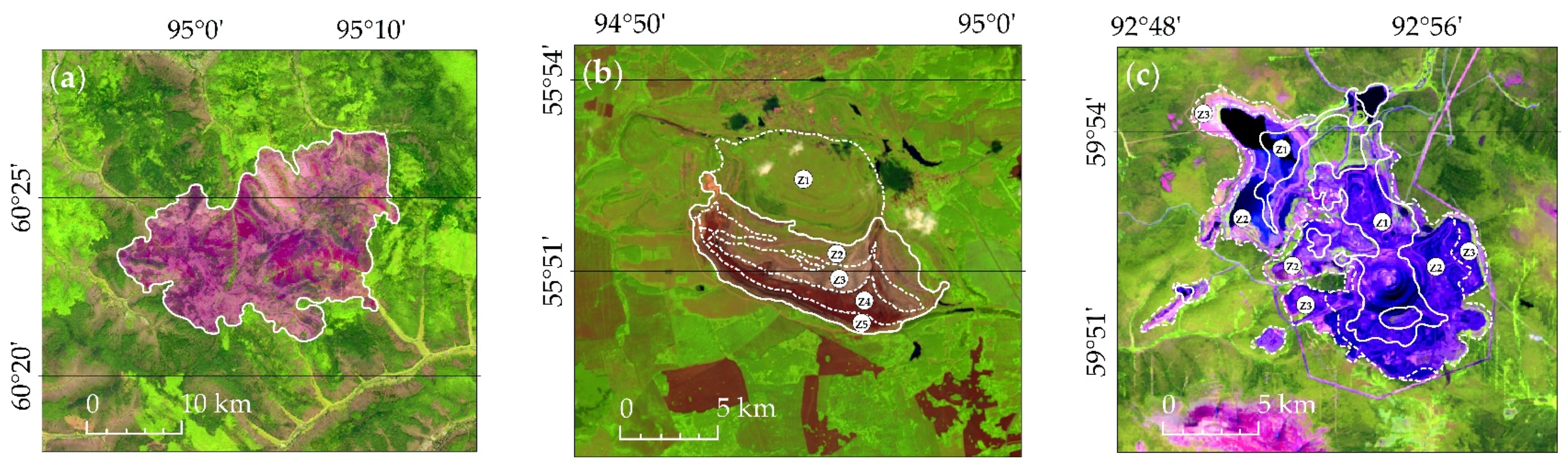
2. Area of Interest and Research Objects

In the current research, we took into account the properties of cryogenic soils, which are typical for the taiga region of Central Siberia (59–66° N, 90–107° E). The forest stands of the region are dominated by larch (Larix sibirica Lebed., Larix gmelinii Rupr. Rupr.) and sparse larch stands, accounting for >50% of the total forested area [26,49,50]. Herb-shrub layer, mosses, and lichens represent the vegetation cover as well as litter loads [51].

The continental climate of the permafrost zone and characteristics of parent rocks determine the genetic specificity of the soils in the region. The soils are characterized by low thickness (0.20–0.50 m) and weak differentiation of the mineral part of the soil profile. The permafrost level (<1.0 m) depends significantly on the topography [11]. Permafrost is widespread on flat areas and is not found in the soil profile on drained areas of slopes and valleys. Periodic freezing and thawing of the soils determine the soil structure, the low rate of humus accumulation in the soil, the peculiarities of moisture transport, and waterlogging. In addition, freezing and thawing processes affect slightly acidic or neutral reaction of the soil, as well as loamy or clayey granulometric composition with a high gravel content in the lower part of the soil profile [49,50]. Finally, cryoturbation, solifluction, cryogenic heaving, thermokarst, etc. characterize such soils.

According to the Russian soil classification of 2004 [52], the soil cover is represented by cryozems (In World Reference Base for Soil Resources (WRB, 2014 [53]) equivalents is Histic Cryosols), podburs (WRB equivalents is Cambic Crysols), and peat soils (WRB equivalents is Cryic Histosols). Cryozems are formed in the lower parts of slopes and microdepressions on rocks of heavy granulometric composition. The soil profile contains a peat litter (thickness of 0.05–0.10 m), a thin humus or coarse humus horizon, and a uniformly mixed cryoturbated mineral horizon with inclusions of plant residues of varying degrees of decomposition. A high (10–14%) humus content characterizes such soils, as the consequence of the low rate of organic matter decomposition. The lower supra-permafrost part of the soil profile is saturated with moisture, structureless, and is more dense and homogeneous. Podburs are formed on fine-earth-clastic products of destruction of metamorphic rocks, which leads to good drainage and to large thickness of the active soil layer. The profile consists of a peat litter, under which lies the Al-Fe-humus horizon, which gradually turns into the parent rock. Peat-cryozems are present in combination with cryozems, located in low relief areas, and are diagnosed by the presence of peat (T) and cryoturbated (CR) horizons.

Background cryogenic soils typically are full-profile, and according to the modern classification [50] have the formula T(Oao)-O(F+H)-CR-C_┴ (Figure 1).

Wildfire impact changes the structural organization of the soil profile. After a wildfire the soil loses its upper horizon, the level of permafrost occurrence decreases, and the soil formula transforms to Opir-O(F+H)pir-CR-C. Under the conditions of high-intensity burning, the profile structure can transform more strongly. Depending on the degree of litter burnout the soil formula changes to O(F+H)pir-CRpir-C or O(H)pir-CRpir-C. Locally, complete burnout of the upper organic horizons of the soil is possible [54]. Upper part of the soil profile, as a rule, have a thin humus-accumulative (underdeveloped) horizon W or a fragmented coarse humus horizon Oao both in case of post-fire mineralization of cryozems and in case of technogenic transforming of soils. Such soils formula is Oao(W)-C.

Evolution of soils after destructive impacts on thermal insulating covers includes an increase in thawing depth, an increase in soil moisture due to thawing of schlieren and wedge ice, an increase in gleying, and cryoturbation processes, and it proceeds under strong influence of succession.

For instance, the effect of post-fire rapid increase in the thawing depth (by 30–100% in the first year after the fire) [34] leads to a unique path of soil evolution, when the underlying gleyed rock layers are included in soil formation for a significant period [55]. This type of evolution is possible only in the permafrost zone. Moreover, an increase in the STL thickness leads to the thawing of schlieren (sometimes wedge ice). An excessive amount of moisture under conditions of difficult drainage stimulates the gleying process [55].

The objects of modeling were (i) native variant, which is undisturbed natural state of cryozem, and (ii) variants of soils with the topsoil layer disturbed as a result of a destructive factor.

The set of input parameters (

Table 1. Input parameters used for numerical simulation of the temperature regime in the soil profile. Physical characteristics of non-disturbed soils, summarized from the works in [49,50,56,57,58,59].

Horizon	Specific Heat, J/(kg·K)	Volumetric Water/Ice Content (Qw) *	Porosity	$\mathbf{Bulk}\mathbf{Density}\mathbf{of}\mathbf{Dry}\mathbf{Soil},{\mathit{\rho }}_{\mathit{b}},\mathbf{kg}/{\mathbf{m}}^3$	Depth, m
Oao	1500	0.3/0.8	0.91	60	0.0–0.12
O(F+H)	1880	0.35/0.79	0.81	70	0.12–0.17
CR	750	0.275/0.3	0.48	1100	0.17–0.35
C	920	0.3/0.33	0.36	1500	0.35–Zend **

* Constant values of the volumetric water/ice content. ** Z_end—maximum depth of computational domains, m.

and

Table 2. Input parameters used for numerical simulation of the temperature regime in the soil profile. Physical characteristics of disturbed soils (post-fire and technogenic impact), summarized from the works in [49,50,56,57,58,59].

Horizon	Specific Heat, J/(kg·K)	Volumetric Water/Ice Content *	Porosity	$\mathbf{Bulk}\mathbf{Density}\mathbf{of}\mathbf{Dry}\mathbf{Soil},{\mathit{\rho }}_{\mathit{b}},\mathbf{kg}/{\mathbf{m}}^3$	Depth, m
O(F+H)pir	1880	0.35/0.79	0.81	70	0.12–0.17
CR (CRpir)	750	0.275/0.3	0.48	1100	0.17–0.35
C	920	0.3/0.33	0.36	1500	0.35–Zend **

* Constant values of the volumetric water/ice content. ** Z_end—maximum depth of computational domains, m.

) for the numerical simulation of the soil temperature regime was summarized from the data of field studies of the morphological and physical properties of soils carried out in the region [49,50,56,57,58,59].

According to field experiments in the permafrost zone [50], “thermal inversion” is possible in different layers of cryogenic soils of disturbed plots. Thus, there is stronger heating of the surface in summer (due to lower thermal resistance). Next, there is a higher temperature in the soil horizons during the non-growing period (early spring, winter, autumn) (due to the higher thermal resistance) in comparison with the distribution in the background plots. During the growing season (summer), such differences are explained by the state (or loss) of disturbed upper soil horizons and the reduced albedo value. The relative change in thermal resistance during the non-growing season can only be explained by a higher ice content in the soils of non-damaged plots, if the snow cover is equal.

As the model used did not consider the transfer of moisture within the soil, values of the volumetric water/ice content were tabulated as constants for the summer and winter seasons (Table 1 and Table 2).

3. Materials and Methods

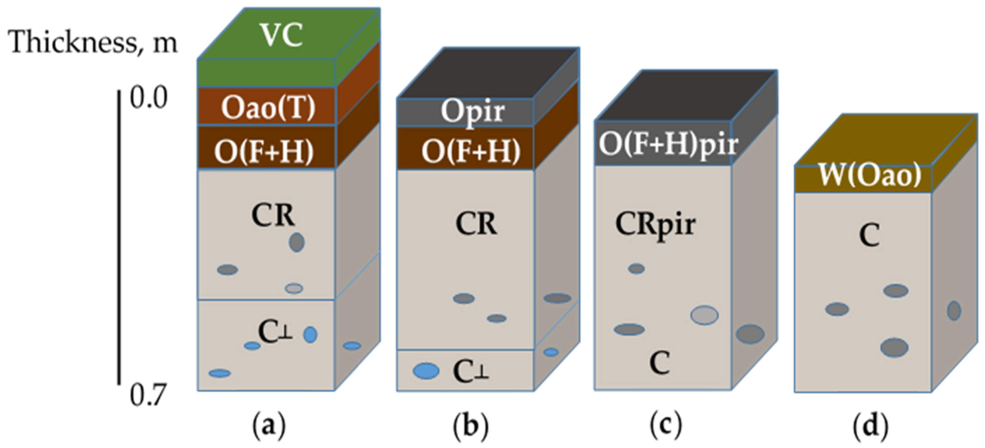
3.1. Multispectral and Infrared Survey of Research Objects

We used satellite images of average spatial resolution (15–30 m) from Landsat-5/7/8 for 1975–2020, which are freely available in The United States Geological Survey (USGS) database (https://earthexplorer.usgs.gov/, accessed on 21 May 2021). The surface temperature was evaluated from the calibrated В6 channel (λ = 10.4–12.5 μm, Landsat-5/TM—Thematic Mapper), B6/1 channel (Landsat-7/ETM—Enhanced Thematic Mapper), and B10 channel (λ = 10.6–11.9 μm, Landsat-8/OLI—Operational Land Imager). We implemented radiometric correction method to the initial data using calibration constants from the metadata files [60,61]. First, we analyzed the availability of the imagery for selected experimental post-technogenic and post-fire plots to obtain time-series for each plot for 1975–2020. The only criteria were the percentage of cloudiness, the binding of the survey dates to the middle of the growing season (July), and the regularity of survey covering of selected objects. Daytime imagery was used only. Thus, we did not implement any special procedure for the selection of Landsat images.

Additionally, we used low spatial resolution survey data (250–1000 m) from Terra/MODIS (Moderate Resolution Imaging Spectroradiometer) for 2002–2020. Standard products L2G and L3 used (free USGS database, https://lpdaac.usgs.gov/dataset_discovery/modis, accessed on 21 May 2021). We operated with reflectances (albedo) measured in MODIS band #1 (λ = 0.620–0.670 μm) and band #2 (λ = 0.841–0.876 μm) (product MOD09GQ), and to analyze surface temperature anomalies we used the MOD11A1 standard product. We used 10-day averaged data across the entire set of initial data, with a special focus on the disturbed ecosystem’s recovery succession stages. A monthly data average procedure, as well as a procedure of spatial averaging within each natural and technogenic disturbed ecosystem plots, were applied.

We have selected the time series of satellite data for two variants of plots with disturbed vegetation and on-ground cover: (1) natural ecosystems of post-fire plots (PF) for 1996–2018 and (2) post-technogenic plots for 1975–2019.

Using time series of satellite data, we performed indirect assessments of the state of disturbed ecosystems (disturbed plots) at different periods of recovery successions based on changes in the anomalies of spectral features comparing to characteristics of the background areas. We analyzed data for 30 post-fire plots recorded in Siberia in 1996, 2006, and 2017 (Figure 2a), and the dynamics of spectral anomalies for two technogenic plots: Borodinsky Coal Mine (BCM) for 1975–2018 and Olimpiada Mining Plant (OMP) for 2000, 2011, 2019 (Figure 2b,c).

We analyzed the dynamics of albedo and temperature anomalies during 1, 5, 10 (or 12), and 20 years of post-fire vegetation and on-ground cover restoration. For technogenic disturbances, we analyzed albedo and surface temperatures during 1, 10, 20, 40, and 60 years after impact a destructive factor on soil covers.

To determine the relative anomalies of the surface temperature of disturbed plots to the characteristics of background territory (ΔT/T_bg (°C/°C), in %), we compared averaging over 10 measurements for each period of recovery:

ΔT/T_bg = 100%·(T_tg—T_bg)/T_bg,

(1)

where T_tg is surface temperature of target (disturbed plot), °C, and T_bg is surface temperature of background (non-disturbed) plot, °C.

3.2. Mathematical Model of Heat Transfer in the Soil

Mathematical models of heat transfer in soils taking into account water-ice phase transformation are quite diverse [62]. The choice of the model depends on the specifics of the problem being solved. Climatological studies often impose severe constraints on the computational resources that can be assigned to calculations of soil heat transfer, therefore analytical and semi-analytical methods are widely used [63,64]. These methods are based on constant or piecewise constant approximations of the main thermophysical characteristics (density, specific heat capacity, and thermal conductivity coefficients) in their dependence on the depth and on the assumption that the temperature depends on the vertical coordinate only.

The formulation of the issue of heat transfer in disturbed cryogenic soil took into account the following factors.

(1)

The multidimensional character of the temperature distribution, being a result of vicinity of disturbed and non-disturbed plots and, accordingly, the presence of a significant difference in the state of the permafrost layer. Under these conditions, significant heat transfer in the horizontal direction can arise.

(2)

Inhomogeneity of the thermophysical properties of the soil, due to the vertical structure of the soil profile and its differences in disturbed and background plots.

(3)

The presence of a transition zone with a mixed phase state of water and ice. Such areas inevitably arise due to local heterogeneities of the soil, its composition, and moisture content. For the used scale of grid sampling in the considered problem, the transition zone is described in terms of the average content of the liquid and solid phases of water.

In a mathematical model of heat transfer in soil, either the temperature field or the specific enthalpy field can be considered as a sought field [65]. The choice of temperature as a sought field is more expedient for the considered problem. This facilitates greatly the process of composition of the thermophysical properties of soil. Thus, the following formulation for the heat transport equation was chosen:

$$c_p\left(x,T\right)\rho \left(x\right)\frac{\partial T}{\partial t}-\frac{\partial }{\partial x_i}\left(\lambda \left(x,T\right)\frac{\partial T}{\partial x_i}\right)=S,$$

(2)

where T is the temperature (K), $c_p\left(T\right)$ is the thermal capacity (J/(kg∙K)), ρ is the density (kg/m³), $\lambda \left(T\right)$ is the thermal conductivity coefficient (W/(m·K)), and S is the heat source associated with the phase change latent heat (W/m³).

Formulating the model of the heat source S, we consider the liquid and solid phases as separate components of the medium. They can present at the same place (i.e., in the same finite volume of the discrete mathematical model) simultaneously. This approach allows taking into account a fine structure of intermitting water and ice that is typical for freezing and thawing soils [66] but cannot be resolved in a discrete model due to the restrictions for a grid dimension. The mass sources of solid and liquid phases are opposite and proportional to the temperature on the Celsius scale [66]. In accordance with the chosen approach, the source term S in Equation (2) has the following form:

$$S=-y_w\left(x,T\right){\rho }_{w}L\frac{\partial {\alpha }_l}{\partial t},$$

(3)

where $y_w$is the soil volumetric content of water regardless to the state (m³/m³), ${\alpha }_l$ is the liquid water fraction, and L is the latent heat (J/kg).

The phase transition rate is determined by the heat transfer flux to the contacts between the phases. This flux is proportional to the difference between the mean temperature of the soil and the phase change temperature, in other words, to the mean temperature of the soil measured in Celsius degrees. Considering the phase transition process as the exponential decay of the diminishing phase, we can write the following equation for the liquid water fraction:

$$\frac{\partial {\alpha }_l}{\partial t}=k(\max \left(T \left[°C\right], 0\right)\left(1-{\alpha }_l\right)+\min \left(T\left[°C\right], 0\right){\alpha }_l),$$

(4)

where $k$ is a coefficient connecting the characteristic timescale of the exponential decay of the diminishing phase and temperature.

Equation (2) was solved in a two-dimensional formulation, in which the vector of coordinate x has vertical and horizontal components (to take into account the effects of the transition region between disturbed and undisturbed soil areas). Large-scale variability of the soil structure and its moisture content, as well as the presence of dynamically changing depth of snow cover, are taken into account in the expressions for the coefficients of the Equation (2): $c_p\left(x,T\right), \rho \left(x\right), \lambda \left(x,T\right), y_w\left(x,T\right)$.

Equation (2) was solved with the use of the finite volume method in that the equation domain is divided into a large number of cells that have four faces as the case is two-dimensional. The sought temperature fields are determined as a set of temperature values at the centers of the cells and the differential Equation (2) is replaced by a system of linear algebraic equations (grid equations) connecting the values at the centers of the cells [67]. Integration of Equation (2) along the cell volumes leads to the algebraic grid equations in that the sought variables are the temperature values in the cell centers [68].

Available models [1,4,5,69,70] were used to derive expressions for the thermal conductivity depending on the vertical coordinate. Empirical models by Pavlov [69], Anisimov et al. [70] are results of the generalization of the great amount of field measurements. In these models, the thermal conductivity coefficient is a function of the dry soil density and the volume fraction of water or ice. The models proposed in the works [1,4,5] are based on the supposition [71] that the thermal conductivity of a partially water-saturated soil correlates linearly with the thermal conductivities of a dry and a water-saturated soil:

$$\lambda =Ke{\lambda }_{sat}+\left(1-Ke\right){\lambda }_d,$$

(5)

where ${\lambda }_{sat}$ and ${\lambda }_d$ are the thermal conductivity coefficients of a soil in the water-saturated and dry states (W/(m·K)), and Ke is Kersten number.

We used the model by Porada et al. [5] for the moss and lichen layer (Oao horizon). For the horizon О(F+H) that consists mainly of medium and well decomposed organic residues, the model by Anisimov et al. was used [70]. For the following two mineral horizons CR and C two types of models were considered [4,69] (

Table 3. Models of thermal conductivity coefficients used for different soil horizons.

Horizon	Models of Thermal Conductivity Coefficients	Parameters Used	Author, Reference
Oao	Equation (5) with ${\lambda }_d=0.05$ and ${\lambda }_{sat}={\lambda }_o{}^{\left(1-\left(w_f+w_s\right)\right)}·{\lambda }_l{}^{w_l}·{\lambda }_s{}^{w_s}$  ${\lambda }_o=0.25;{\lambda }_l=0.56;{\lambda }_s=2.25$	${\lambda }_d$ is the thermal conductivity of dry organic substance, ${\lambda }_o$ is the thermal conductivity of the organic substance in the water-saturated condition, w is the volumetric fraction of a certain state of water, s is the solid state of water, l is the liquid state of water.	Porada et al., 2016 [5]
O(F+H)	${\lambda }_t=0,08·e^{3.88w_f}$  ${\lambda }_{fr}=\left(615w_s+22.2\right)·{10}^{-3}$	$t$ is the thawed soil, fr is the frozen soil	Anisimov et al., 2012 [70]
CR	$\lambda =k\left(0.001·{\rho }_b+{10}^4·w/{\rho }_b-1.1\right)-1.16·{10}^4·w/{\rho }_b$ Equation (5) was used, where ${\lambda }_{sat}={\lambda }_o{}^{\left(1-\left(w_f+w_s\right)\right)}·{\lambda }_f{}^{w_f}·{\lambda }_i{}^{w_i}$  ${\lambda }_d=\left(A·{\rho }_b+B\right)/\left({\rho }_{soil}+C·{\rho }_b\right)$ Coefficients A, B, С, D summarized from [1,4]	${\rho }_b$ is the bulk density of dry soil; ${\rho }_{soil}$ is the density of the material of soil particles; w is the volumetric water/ice fraction; k is the empiric coefficient specific for the type and condition of soil	Pavlov, 1979 [69], Ekici et al., 2014 [4], Tarnawski et al., 2000 [1]

). In calculations relating to periods with stable snow cover the thermal conductivity of snow was admitted to be a constant, ${\lambda }_{snow}$ = 0.23 W/(m·K).

Other thermophysical properties of snow (density, heat capacity, and albedo) were also assumed to be constant, but the depth of the snow cover was considered as alternating according to meteorological data.

The boundary conditions at the upper boundary of a soil or snow take into account the presence of solar (shortwave) and atmospheric (longwave) radiation and convective heat transfer by air [72,73]:

$$-\lambda \left(\frac{\partial T}{\partial x}\right)=q_c+\left(1-{\alpha }_s\right)·q_{Sr}+q_{Lr},$$

(6)

where $q_c$ is the convective heat flux, $q_{Sr}$ and $q_{Lr}$ are the shortwave and longwave radiation heat fluxes, and α_s is the surface albedo.

The surface convective heat flux is calculated with the use of the following expression [69]:

$$\begin{array}{c}{q}_c=a_s·\left(T_{atm}-T_s\right),\\ {\alpha }_s=u_1^{0.5}·\left(6+3.1·\Delta T/u_1^2\right)\end{array}$$

(7)

where ${\alpha }_s$ is the heat transfer coefficient, W/(K∙m²); $u_1$ is the wind velocity at the altitude 1 m; and $\Delta T$ is the temperature difference between the solid surface and atmosphere.

The shortwave radiation heat flux divides into the direct solar radiation $\left(I_{Si}^{Dir}\right)$ and the scattered one $\left(I_{Si}^{Dif}\right)$:

$$q_{Sr}=q_{Sr}^{Dir}+q_{Sr}^{Dif},$$

(8)

The direct solar heat flux on a horizontal surface is found as [47]

$$q_{Sr}^{Dir}=q_{Sr0}·\cos Z·{{\displaystyle \prod }}_i{\tau }_i,$$

(9)

where Z is the reduced incidence angle, ${\tau }_i$are the atmosphere transmittance factors that characterize absorption by aerosols, water vapor, ozone, other gases, and Rayleigh scattering; $q_{Sr0}$ (W/m²), is the Solar heat flux reaching the Earth atmosphere. The value of $q_{Sr0}$ depends on the position of the Earth relative to the Sun [73]. The factors ${\tau }_i$ in (9) are calculated according to [47].

Contributions to the scattered radiation flux are made by the Rayleigh and aerosol scattering and multiple reflection of the direct solar radiation. The meteorological data for cloud cover were used to calculate the change in relative insolation.

Longwave radiation heat exchange between the solid surface and the atmosphere is calculated as

$$q_{Lr}={\epsilon }_s·\left({\epsilon }_{atm}\sigma ·T_{atm}^4-\sigma ·T_s^4\right),$$

(10)

where${\epsilon }_s$ is the surface emissivity and ${\epsilon }_{atm}$ is the atmosphere emissivity. For the surface of the damaged and undamaged soil, the values of the integral albedo were taken equal to 0.13 and 0.18 (a decrease by 40% for the case of a significant change in the state of the ground cover and the upper organic horizon), the emissivity values are 0.9 and 0.98, respectively [74]. The atmosphere emissivity ${\epsilon }_{atm}$ was calculated as a function of cloud cover and humidity [75,76].

3.3. Meteorological Data

We used long-term series of meteorological information from open data banks for the period 1990–2020: Climatic Research Unit (http://www.cru.uea.ac.uk/, accessed on 25 March 2021), Weather archive (http://rp5.ru, accessed on 25 March 2021), and the National Climatic Data Center (NCDC) (http://www7.ncdc.noaa.gov/CDO/cdo, accessed on 25 March 2021).

To calculate solar heat flux (4), we used the geographic coordinates of Tura (64° N, 100° E) (Evenkia, Krasnoyarsk region, Siberia, Russia). The data on the depth of snow cover (mm), air temperature (°C), wind speed (m/s), and cloudiness (oktas) were taken from the annual series of meteorological data. The observations have a regularity of 4 h (6 times a day). Numerical simulations are performed for 2018 data (Table S1, Supplementary Materials).

3.4. Main Features and Assumptions of the Mathematical Model of Heat Transfer in the Soil

The governing equations of the mathematical model are (1) and (4), that describe heat transfer in soil in presence of water-ice phase transition neglecting the moisture transfer processes. The main thermophysical properties, in addition to thermal conductivity, were set constant for different soil horizons, but different for temperatures above and below 0 °C. The calculations were performed for a time interval up to three years required to establish a quasiperiodic solution.

The result of the numerical solution of the model equations was the dynamics of two-dimensional temperature fields and phase transition boundaries.

In the mathematical model, the discretization of the computational domain was built based on a Cartesian (orthogonal, structured) grid. The vertical grid step was 0.01 m, the horizontal one was from 0.25 m, and the time step was 15 min.

In the mathematical model, the boundaries of the soil horizons were assumed constant and dynamic change of the snow cover depth according to the data of meteorological observations was taken into account. A linear temperature distribution changing from the air temperature at the surface to the specified temperature at the lower boundary (Z_end) (see Table 1 and Table 2) of the equations domain was assumed as the initial temperature distribution in the soil.

4. Results

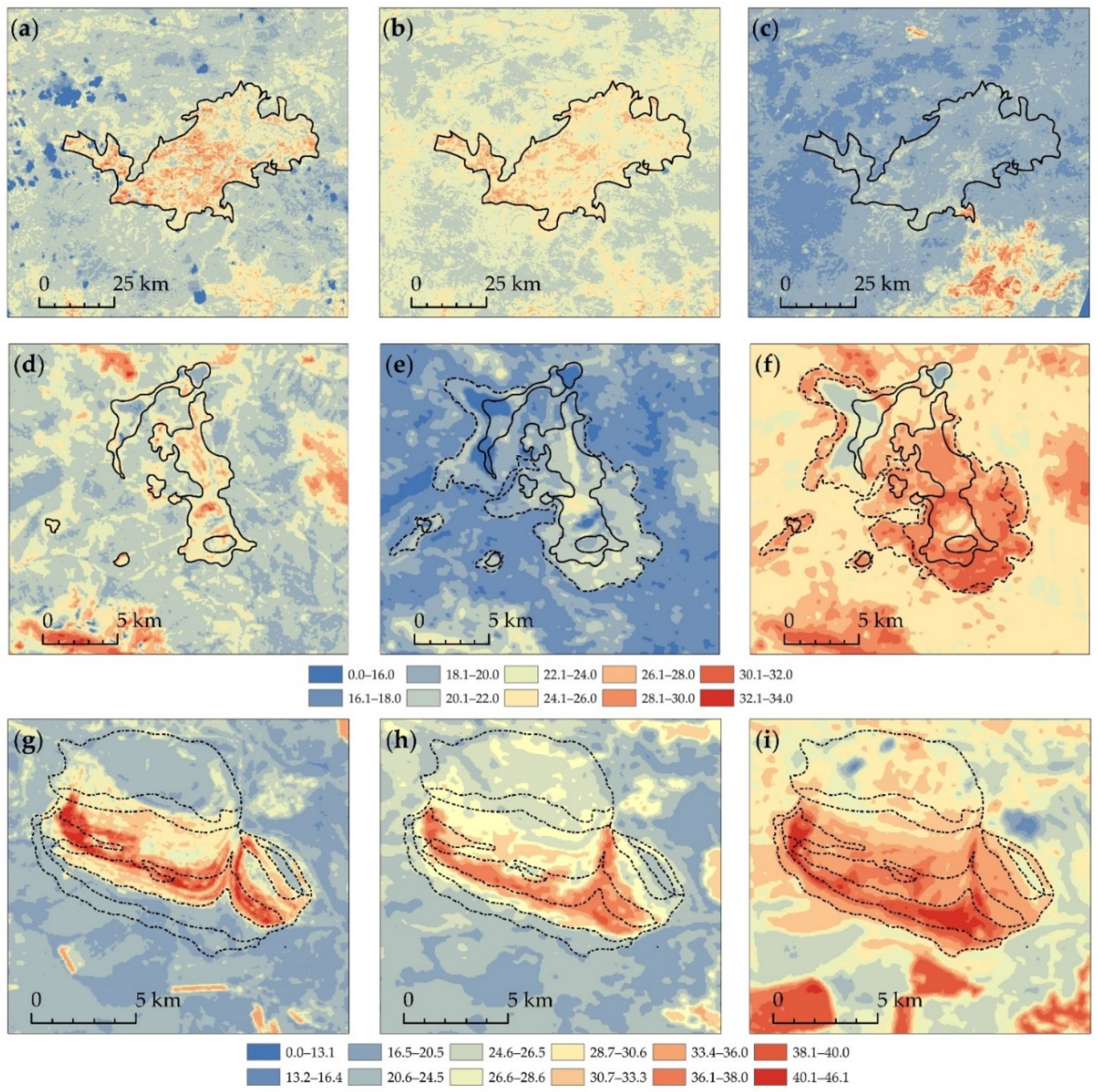
4.1. Surface Temperature Anomalies of Disturbed Plots on Satellite Data in IR Range

Time series of satellite imagery reflect the change in spectral characteristics and temperature anomalies of disturbed areas caused by recovery of vegetation and of a ground cover (Figure 3). For PF plots it was evaluated for the period of 20 years, for both BCM and OMP plots it was analyzed for the period of >60 years. The peculiarity of plots after fire disturbances is that natural recovery processes occur there. The peculiarity of post-technogenic plots is that there are two possible options for dynamics of the ecosystem: (1) restoration after reclamation or (2) long-term condition in the format of non-reclaimed lands (dumps, mineralized surfaces). Each of these options is of interest from the point of view of the formation of surface temperature anomalies and its effect on the properties of soil horizons.

The long-term dynamics of spectral albedo (α) and surface temperature anomalies in disturbed plots of natural and technogenic landscapes in comparison with the background data are summarized in

Table 4. Changes in the spectral characteristics of disturbed areas in % to background values for the options PF, BUR (reclamation), and OMP (without reclamation). Mean value for July ± SD, p < 0.05.

Recovery Time, Years	Albedo Decreasing (%) λ = 0.620–0.670 μm		Albedo Decreasing (%) λ = 0.841–0.876 μm		ΔT/Tbg (%) λ = 10–12 μm
	PF/BCM (Reclamation)	OMP (without Reclamation)	PF/BCM (Reclamation)	OMP (without Reclamation)	PF	BCM (Reclamation)/OMP (without Reclamation)
1	17.5 ± 4.8	53.1 ± 11.3	48.5 ± 1.5	46.8 ± 5.2	28.5 ± 3.4	77.9 ± 10.4
5	16.9 ± 5.6	–	27.5 ± 3.6	–	15.0 ± 2.5	–
10–12	15.4 ± 5.5	50.6 ± 8.1	25.0 ± 3.7	51.4 ± 5.6	12.5 ± 1.1	55.0 ± 8.3
22	3.1 ± 0.2	62.9 ± 13.9	12.5 ± 1.1	50.2 ± 5.5	3.6 ± 0.6	43.0 ± 6.2
30	–	–	–	–	–	32.4 ± 4.5
>40	–	–	–	–	–	18.7 ± 0.3

The data obtained for the two considered channels of satellite equipment (two spectral ranges) (Table 4) correspond to the change in the integral albedo of the disturbed plots [74] incorporated in the model of current research as one of the input parameter.

.

4.2. The Results of Numerical Simulation

The direct results of numerical simulation are dynamics of fields of temperature and fraction of liquid and solid states of water, radiation, and convective heat flux on the surface (Table S2, Supplementary Materials). The phase transition boundary and the magnitude of the relative surface temperature anomaly for disturbed areas in comparison with the background ones are the indicators most important for analysis.

Figure 4a shows the formation of a periodic solution during a three-year calculation period. Figure 4b demonstrates the differences in the dynamics of the phase transition boundary for damaged and undamaged soils. Figure 4c shows the dynamics of the surface temperature anomaly in the summer months through the values of the relative temperature deviation (ΔT/T_bg, °C/°C) from background values. Figure 4d reveals the influence of the season and optical properties of the surface (soil or snow) on the annual dynamics of the total radiation flux.

The influence of changes in the optical properties and moisture content of disturbed soil areas on the formation of thermal anomalies in the numerical simulation results are shown in

Table 5. Moisture content and albedo in the variants of model problem statement and calculated values of ΔT/T_bg for summer. Moisture content and albedo are given for disturbed/non-disturbed plots.

Horizon	Volumetric Water Content	Albedo for Disturbed Plot/Background	ΔT/Tbg, %
Var. 1. Basic set of conditions
Oao	–/0.6	0.13/0.18	15–25
O(F+H)	0.35/0.14
Var. 2. No change in the moisture content for the horizon O(F+H)
Oao	–/0.6	0.13/0.18	7–12
O(F+H)	0.35/0.35
Var. 3. Equal moisture content in the upper soil horizons
Oao	–/0.6	0.13/0.18	<5
O(F+H)	0.35/0.6
Var. 4. Moisture content similar to Var. 3 with greater change in albedo
Oao	–/0.6	0.07/0.28	10–25 (mean ~15%)
O(F+H)	0.35/0.6

. Several variants of the set of soil conditions were examined. One of them was considered as the basic set of conditions (Table 1 and Table 2) and others differed from it in a certain parameter value in order to reveal the influence of this parameter. We considered the following variants: (i) basic set of conditions, (ii) no change in the moisture content for the horizon O(F+H), (iii) equal moisture content in the upper soil horizons, and (iv) moisture content similar to var. 3 with greater change in albedo. In the cases considered, ΔT/T_bg varied from 5 to 25%.

5. Discussion

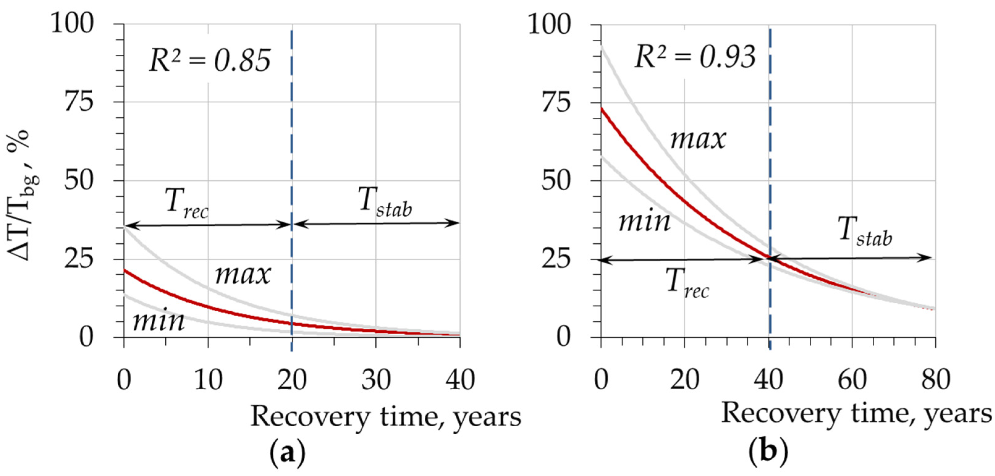
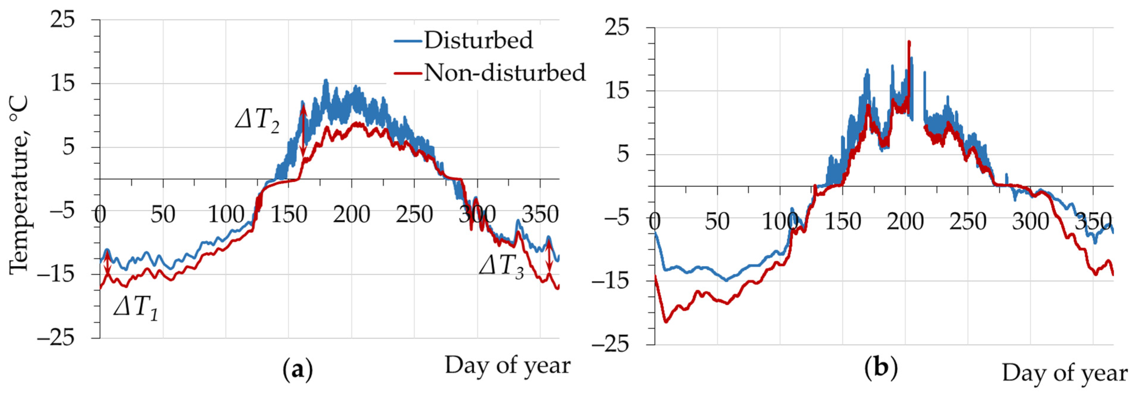
5.1. Long-Term Surface Temperature Anomalies

Temperature anomalies in the post-fire areas are typical for permafrost conditions of Siberia [11,12,56].

A decrease in the spectral and broadband albedo (α, %) of the surface in post-fire areas, due to partial or complete combustion of the ground cover, provokes excessive heating of the surface. As shown by the remote measurements (Table 4), the spectral albedo in the short-wavelength bands (MODIS band #1 and #2) is reduced by 20–48% relative to the background immediately after the fire, by 15–25% after 10 years of recovery, and by 3–12% after 20 years of vegetation regeneration. For the variant of post-technogenic plot BCM (with reclamation), the albedo values correspond to the dynamics in PF, while for OMP (dumps without reclamation) the level of the albedo reduction remained 45–60% throughout the observation period (Table 4).

Under conditions of positive air temperatures in summer, as well as in spring and early-autumn, the effect of significant surface temperature anomalies (ΔT/T_bg, %) was recorded in all variants of the disturbed plots (PF, BCM, OMP) in comparison with background surface temperature.

In PF plot ΔT/T_bg on average reaches values of 33 ± 6% with maxima of ~46%, which were recorded immediately after fire impact. During 10–12 years, on average, the value of the temperature anomaly decreases to ~12.5 ± 1% (sporadic maxima ~20%). During at least 20 years (the stabilization time lag T_stab, Figure 5a), the anomaly amplitudes decrease to the level of background values and the measurement error of 3 ± 1% (Table 4, Figure 5a). Thus, during the period under consideration, stabilization of temperature parameters is observed in PF plot, which is determined by the thermal insulation properties of the surface layer recovering to the pre-fire state under conditions of a successful vegetation regeneration [11,34,56,77].

The considered post-technogenic plots were characterized by a higher level of initial relative surface temperature anomalies (up to 100% of the background). Further, an exponential decrease was observed, similar to PF plot (R² = 0.87–0.92) (Figure 5). However, the stabilization time lag (T_stab) is 40–60 years, which is characterized with ΔT/T_bg of 18–20% under the conditions of recovery (Figure 5b).

A significantly high level of ΔT/T_bg in technogenic areas remains twice as long as in PF plot. In disturbed ecosystems, the morphological and physical properties of the upper soil horizons are not restored to the background level for a long time [56,78]. Thermal regimes remain significantly anomalous for up to 60–80 years (Figure 5b). Even after the time of stabilization (T_stab > 60 years), the level of relative anomaly overestimated at least by 15–20% in relation to the background values. Probably, we can talk about “neo-technogenic ecosystems” forming, which are characterized by special thermal regimes of soils that differ from the background ones both for reclamated (BCM) and for non-reclamated (OMP) plots. The main reason for such changes is a significant mechanical effect on the soil and/or complete destruction of its structure, which restoration requires much longer time.

These results can be explained by the fact that mechanical reclamation cannot provide an increase in the rate of restoration of the state of the litter and upper soil horizons to the level of the background territories. Although, the restoration of vegetation (as a factor that changes the albedo) proceeds faster in reclaimed areas, where successions acquire a character closer to natural restoration processes.

The formation of thermal anomalies in disturbed plots can be caused by a sharp change in three factors (i) surface emissivity, (ii) albedo, and (iii) moisture content in the upper soil horizons.

Surface emissivity determines the heat loss due to the re-emission of absorbed short-wave solar radiation into the atmosphere. The coefficient of surface emissivity decreases in the disturbed plots [74,77]. However, heat losses from the surface with damaged vegetation and soil cover at significant ΔT/T_bg should be higher than from the undisturbed surface, due to the strong nonlinear dependence of thermal radiation on temperature (according to Stefan–Boltzmann law). Consequently, heat losses contribute to a decrease in ΔT/T_bg values. Thus, the surface emissivity does not fully determine the formation of thermal anomalies.

According to field observations conducted in the study area [7,50], changes in albedo and moisture content conditions can also contribute to the formation of thermal anomalies.

The spectral albedo of disturbed areas in all variants (PF, BCM, OMP) significantly differs from the background values (Table 4). At the initial stages (during the first years after the destructive factor impact), this factor significantly affects the absorption of solar radiation. However, it is numerically shown (Table 5) that the albedo reduction by 45–55% leads to a decrease in the proportion of absorbed solar radiation by <10%, and only by 6% for the model of “native” variant (see Table 5).

In addition to changing the optical properties in disturbed areas, conditions are formed for changing the water content in the near-surface soil horizons [35]. Such changes in moisture content directly depend on the degree of disturbance of the vegetation cover and soil, including the disturbance of its structural organization. Probably, it is this parameter that determines thermal anomalies and their presence at later stages of recovery processes (10–20 years in PF plots or >60 years in BCM and OMP), when the spectral albedo and the surface emissivity are leveled as a result of the restoration of vegetation and litter cover. It was previously shown [27,79] that vegetation signs are restored no later than 7 years after a wildfire. Nevertheless, a change in the soil moisture regime in disturbed plots provokes a decrease in the thermal conductivity of the upper soil horizons. We believe that this is the main reason for the existence of significant temperature anomalies even after the normalization of the optical properties (albedo, surface emissivity) of the disturbed ecosystems.

5.2. Results of Numerical Simulation of the Annual Dynamics of Heat Transfer

As the results of the numerical simulation show, the initial temperature distribution is changed by a periodically time-dependent one starting from the second year. At a depth of 0.1 m, this change occurs after five months (Figure 4a).

At the beginning of the negative air temperatures period a thawed cavity is formed, surrounded by frozen soil in the area above the permafrost zone (Figure 4b). It decreases on both upper and lower sides. This phenomenon exists for 14 days in the non-disturbed soil, and up to 21 days in the soil of the damaged plot. Freezing in the intact soil starts two weeks later than in the soil of the damaged plot.

The maximum inflow and losses of heat due to longwave and shortwave radiation occur in summer and amount to about 350 and 100 W/m², respectively (Figure 4d). Heat loss in summer occurs mostly during nights. In winter, with a high snow albedo, the soil loses 30–50 W/m² due to radiation (Figure 4d). Abrupt changes in the profile of the radiation flux are associated with snowfalls and melting of snow, which affects the surface albedo sharply.

The numerical solution shows a positive temperature anomaly ΔT/T_bg = 15–25% in the damaged areas in summer (Table 5, var. 1), which correlates with the data of satellite observations (Table 4, Figure 5), in particular for the post-fire areas (PF). Such values of ΔT/T_bg are achieved in the case of a simultaneous significant decrease in moisture content and a change in the optical characteristics of damaged areas.

The simulation results demonstrate that a significant role in the formation of the temperature anomaly belongs to the change in moisture content. When the influence of the moisture content factor is excluded, the effect of changing in the radiant flux does not exceed ΔT/T_bg = 5% (Table 5, var. 3) that is 4–5 times less than data from remote sensing. With a decrease in moisture content for the upper soil horizon to the level of the second soil horizon of the non-disturbed soil, ΔT/T_bg becomes two times higher but remains below the observed values (Table 5, var. 2). Only with further 2.5 times decrease in the moisture content (Table 5, var. 1), the simulation results correlate with the data of satellite observations. To reproduce the observed thermal anomaly in the mathematical model changing only the amount of the absorbed radiation, the albedo in the disturbed area must be several times less than in the undisturbed areas (Table 5, var. 4).

5.3. Thermal Inversion

Thermal inversion in soil temperature values in comparison of disturbed and undisturbed areas was observed both in numerical simulation (Figure 6a) and in field measurements (Figure 6b) [50]. The results of numerical simulation allow us to state that the condition for this effect is a higher ice content in the soils of the background areas, in comparison with the variants of disturbed territories.

Due to the higher ice content, despite the presence of the heat-insulating soil horizon Oao, the temperature in the soil of non-disturbed plots decreases faster (Table 3 [5,70]). In the summer, the opposite situation is realized. Greater heating of soils in disturbed plots causes an increase in the depth of the active layer by ΔZ = 29% according to the results of numerical modeling (Figure 4b) in comparison with the background areas, both due to the absence of an additional thermal insulating horizon and due to lower albedo and emissivity values. The calculated increase in thawing depth for disturbed soil is consistent with observational data, which show the magnitude of the relative increase in thawing depth in the range of 25–40% [34].

Comparison of the results of modeling and field observations (Figure 6a,b) shows the similarity of heat transfer processes: thermal inversion, similar nature of temperature dynamics at a depth of 0.1 m for soils of disturbed and background areas. The most significant differences are observed in the summer period (in general, the maxima are higher by about 5 °C), which can be explained by differences in meteorological conditions and model assumptions of soil characteristics (Table 1 and Table 2) that differ from natural ones. In particular, in the presented results for the mineral horizon CR clayey granulometric composition, the model from [69] was used, as the model from the works in [1,4] led to a significant overestimation of the depth of soil thawing [34]. The necessity to refine the model coefficients in accordance with the characteristics of natural soils is obvious.

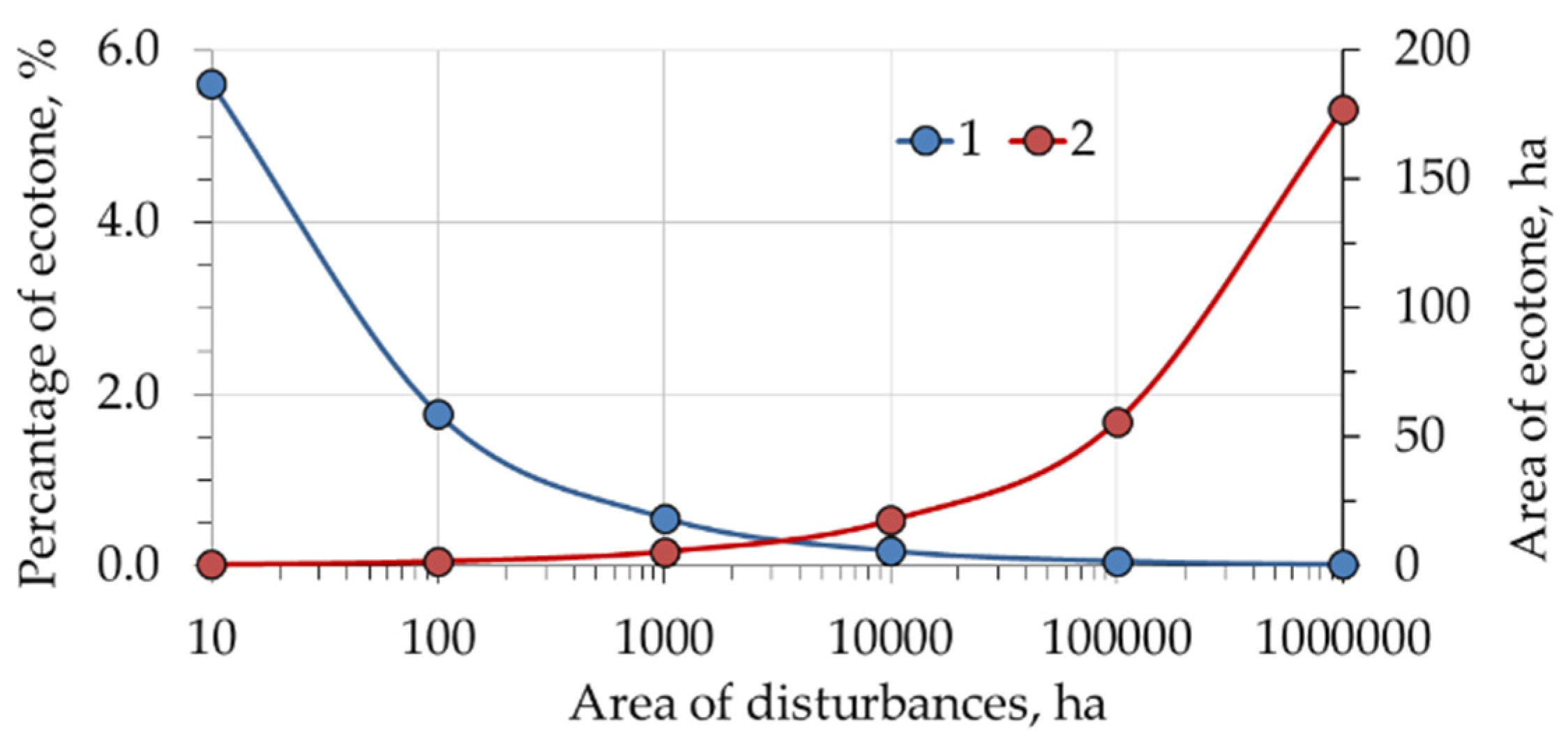
5.4. Transition Zone

The problem of heat transfer simulation is two-dimensional due to boundary effects at the periphery of the damaged plots. The calculated two-dimensional distribution of the temperature field in the summer and autumn months (Figure 7) indicates that at a depth of up to 0.5 m (within the root-inhabited layer), the horizontal propagation of thermal disturbances from plots with damaged soil cover to a non-damaged area can reach ~5.5 m.

Transferring the modeling results to post-fire and post-technogenic disturbed ecosystems, it should be taken into account that along the boundary of disturbed plots, transitional zones (or “ecotones”) (in terms of thermal and moisture conditions) are formed. Their characteristic width is up to ~5 m and area can be up to 6% of the area of the disturbed plots (Figure 8).

The zones formed along the border of disturbed areas should also be considered as transitional zones or “ecotones” characterized by “edge effect”, where conditions favorable for vegetation and biota can develop in the root-inhabited layer of the soil. This factor can be favorable for conditions of vegetation and biota earlier exit from the winter state due to increased temperatures in the root-inhabited layer, which is confirmed for Siberia by field studies [9,10,13,56]. As an ecological factor, this can determine an increase in the density of some populations and be a zone of additional introduction of plant, microbial, and animal communities into the disturbed plots territory [80].

6. Conclusions

Under conditions of the same insolation, plots with disturbances in the upper soil horizons and ground cover are accompanied by the formation of long-term surface temperature anomalies. Similar processes were recorded for both natural (post-fire) and post-technogenic landscapes. Within 20 years, the thermal insulation properties of the vegetation recover in the post-fire areas. Thus, the relative temperature anomaly reaches the level of the mathematical error of measurement. In post-technogenic plots, conditions are more “contrast” compared to the background, and the processes of restoration of the thermal regime take a longer period (>60 years). “Neo-technogenic ecosystems” are formed, characterized with special thermal regimes of soils that differ from the background ones both for reclamated (BCM) and for non-reclamated (OMP) plots.

Along with a change in the optical properties of the surface (the spectral and the broadband albedo, the emissivity coefficient), the main reason for the increased surface and soil temperatures of disturbed plots is a decrease in moisture content in the upper soil horizons. Probably, it is this parameter that determines thermal anomalies in disturbed plots as well as their presence at later stages of recovery processes for 10–15 years after a fires impact and for >60 years in post-technogenic ecosystems of Siberia. Thus, monitoring of surface thermal anomalies can be used as a diagnostic criterion of post-technogenic ecosystems state in the context of territories development after technogenic impacts. The data on the moisture content change in the damaged areas are crucially important for the numerical studies of the temperature profiles evolution. However, these data cannot be obtained directly by the remote observation. Further work on this topic involves not only field measurements of moisture content, but also taking into account moisture transfer in a mathematical model.

The destruction of the upper soil layer and the complete degradation of the moss–lichen cover leads not only to increased surface temperatures in summer, but also causes thermal inversion in soil temperature in winter when the thermal resistance in the upper organic layer of the disturbed plots becomes less than in the upper organic horizons of the background soil. This factor can be favorable for the formation of conditions for an earlier exit from the winter state of vegetation and biota due to the increased temperatures of the root-inhabited layer, which is confirmed for Siberia by field studies [9,10,13,56].

The simulation results show the formation of transition zones (“ecotones”) along the periphery of the disturbed plots due to horizontal heat transfer. The typical size of such a zone is ~5.5 m, and the area is up to 6% of the area of disturbed plots. Probably, zones of rapid recovery successions can form along the boundaries of disturbed areas, which makes further study of their properties urgent.

References

1. Tarnawski, V.R.; Leong, W.H.; Bristow, K.L. Developing a temperature-dependent Kersten function for soil thermal conductivity. Int. J. Energy Res. 2000, 24, 1335–1350. [Google Scholar] [CrossRef]
2. Dankers, R.; Burke, E.J.; Price, J. Simulation of permafrost and seasonal thaw depth in the JULES land surface scheme. Cryosphere 2011, 5, 773–790. [Google Scholar] [CrossRef] [Green Version]
3. Desyatkin, R.V.; Desyatkin, A.R.; Fedorov, P.P. Temperature regime of taiga cryosoils of Central Yakutia. Kriosf. Zemli Earth Cryosphere 2012, 16, 70–78. (In Russian) [Google Scholar]
4. Ekici, A.; Beer, C.; Hagemann, S.; Boike, J.; Langer, M.; Hauck, C. Simulating high-latitude permafrost regions by the JSBACH terrestrial ecosystem model. Geosci. Model Dev. 2014, 7, 631–647. [Google Scholar] [CrossRef] [Green Version]
5. Porada, P.; Ekici, A.; Beer, C. Effects of bryophyte and lichen cover on permafrost soil temperature at large scale. Cryosphere 2016, 10, 2291–2315. [Google Scholar] [CrossRef] [Green Version]
6. Pavlov, A.V. Cryolithozone Monitoring; The Academic Publishing House “GEO”: Novosibirsk, Russia, 2008; p. 229. (In Russian) [Google Scholar]
7. Orgogozo, L.; Prokushkin, A.S.; Pokrovsky, O.S.; Grenier, C.; Quintard, M.; Viers, J.; Audry, S. Water and energy transfer modeling in a permafrost-dominated, forested catchment of Central Siberia: The key role of rooting depth. Permafr. Periglac. Process. 2019, 30, 75–89. [Google Scholar] [CrossRef]
8. Brown, J.; Ferrians, O.J.; Heginbottom, J.A.; Melnikov, E.S. Circum-Arctic Map of Permafrost and Ground Ice Conditions; National Snow and Ice Data Center, Digital Media: Boulder, CO, USA, 2002; Available online: https://nsidc.org/data/ggd318 (accessed on 1 June 2021).
9. Knorre, A.A.; Kirdyanov, A.V.; Prokushkin, A.S.; Krusic, P.J.; Büntgen, U. Tree ring-based reconstruction of the long-term influence of wildfires on permafrost active layer dynamics in Central Siberia. Sci. Total Environ. 2019, 652, 314–319. [Google Scholar] [CrossRef] [PubMed] [Green Version]
10. Kirdyanov, A.V.; Prokushkin, A.S.; Tabakova, M.A. Tree-ring growth of Gmelin larch in the north of Central Siberia under contrasting soil conditions. Dendrochronologia 2013, 31, 114–119. [Google Scholar] [CrossRef]
11. Dymov, A.; Abakumov, E.; Bezkorovaynaya, I.; Prokushkin, A.; Kuzyakov, Y.; Milanovsky, E. Impact of forest fire on soil properties (Review). Theor. Ecol. 2018, 4, 13–23. [Google Scholar] [CrossRef]
12. Zhang-Turpeinen, H.; Kivimäenpää, M.; Aaltonen, H.; Berninger, F.; Köster, E.; Köster, K.; Menyailo, O.; Prokushkin, A.; Pumpanen, J. Wildfire effects on BVOC emissions from boreal forest floor on permafrost soil in Siberia. Sci. Total Environ. 2020, 711, 134851. [Google Scholar] [CrossRef] [PubMed]
13. Kirdyanov, A.; Saurer, M.; Siegwolf, R.; Knorre, A.; Prokushkin, A.S.; Churakova, O.; Fonti, M.V.; Büntgen, U. Long-term ecological consequences of forest fires in the continuous permafrost zone of Siberia. Environ. Res. Lett. 2020, 15, 034061. [Google Scholar] [CrossRef]
14. Anisimov, O.A. Potential feedback of thawing permafrost to the global climate system through methane emission. Environ. Res. Lett. 2007, 2. [Google Scholar] [CrossRef]
15. Anisimov, O.A.; Sherstiukov, A.B. Evaluating the effect of environmental factors on permafrost in Russia. Kriosf. Zemli. Earth Cryosphere 2016, 2, 78–86. (In Russian) [Google Scholar]
16. Masyagina, O.V.; Menyailo, O.V. The impact of permafrost on carbon dioxide and methane fluxes in Siberia: A meta-analysis. Environ. Res. 2020, 182, 109096. [Google Scholar] [CrossRef] [PubMed]
17. Arkhangelskaya, T.A. The Thermal Regime of Soils; GEOS: Moscow, Russia, 2012; p. 282. (In Russian) [Google Scholar]
18. Trofimova, I.E.; Balybina, A.S. Regionalization of the West Siberian Plain from thermal regime of soils. Geogr. Nat. Resour. 2015, 3, 27–38. [Google Scholar] [CrossRef]
19. Goncharova, O.Y.; Matyshak, G.V.; Bobrik, A.A.; Moskalenko, N.G.; Ponomareva, O.E. Temperature regimes of northern taiga soils in the isolated permafrost zone of Western Siberia. Eurasian Soil Sci. 2015, 48, 1329–1340. [Google Scholar] [CrossRef]
20. Koronatova, N.G.; Mironycheva-Tokareva, N.P.; Solomin, Y.R. Thermal regime of peat deposits of palsas and hollows of peat plateaus in Western Siberia. Kriosf. Zemli. Earth Cryosphere 2018, 6, 15–23. (In Russian) [Google Scholar] [CrossRef]
21. Park, H.; Launiainen, S.; Konstantinov, P.Y.; Iijima, Y.; Fedorov, A.N. Modeling the Effect of Moss Cover on Soil Temperature and Carbon Fluxes at a Tundra Site in Northeastern Siberia. J. Geophys. Res. Biogeosci. 2018, 123, 3028–3044. [Google Scholar] [CrossRef]
22. Krasnoshchekov, Y.N.; Sorokin, N.D.; Bezkorovainaya, I.N.; Yashikhin, G.I. Genetic peculiarities of Northern Taiga soils in the Yenisei region of Siberia. Eurasian Soil Sci. 2001, 34, 12–20. (In Russian) [Google Scholar]
23. Prokushkin, S.G.; Abaimov, A.P.; Prokushkin, A.S. Structural and Functional Characteristics of the Gmelin Larch in the Permafrost Zone of Central Evenkia; IL SB RAS: Krasnoyarsk, Russia, 2008; p. 164. ISBN 978-5-903055-13-5. (In Russian) [Google Scholar]
24. Galenko, E.P. Thermal regime formation of soils in coniferous ecosystems of boreal zone in reference to dominating tree species and forest type. Proc. Komi Sci. Cent. Ural. Div. Russ. Acad. Sci. 2013, 1, 32–37. (In Russian) [Google Scholar]
25. Ehrenfeld, J.G.; Ravit, B.; Elgersma, K. Feedbacks in the plant-soil system. Annu. Rev. Environ. Resour. 2005, 30, 75–115. [Google Scholar] [CrossRef] [Green Version]
26. Kharuk, V.I.; Ponomarev, E.I. Spatiotemporal characteristics of wildfire frequency and relative area burned in larch-dominated forests of Central Siberia. Russ. J. Ecol. 2017, 48, 507–512. [Google Scholar] [CrossRef]
27. Ponomarev, E.I.; Ponomareva, T.V. The Effect of Postfire Temperature Anomalies on Seasonal Soil Thawing in the Permafrost Zone of Central Siberia Evaluated Using Remote Data. Contemp. Probl. Ecol. 2018, 11, 420–427. [Google Scholar] [CrossRef]
28. Kharuk, V.I.; Ponomarev, E.I.; Ivanova, G.A.; Dvinskaya, M.L.; Coogan, S.C.; Flannigan, M.D. Wildfires in the Siberian taiga. Ambio 2021, 1–22. [Google Scholar] [CrossRef]
29. Krasnoshchekov, K.V.; Dergunov, A.V.; Ponomarev, E.I. Evaluation of underlying surface temperature maps on logging sites using Landsat data. Sovrem. Probl. Distantsionnogo Zondirovaniya Zemli Iz Kosm. 2019, 16, 87–97. [Google Scholar] [CrossRef]
30. Uzarowicz, Ł.; Charzyński, P.; Greinert, A.; Hulisz, P.; Kabała, C.; Kusza, G.; Kwasowski, W.; Pędziwiatr, A. Studies of technogenic soils in Poland: Past, present, and future perspectives. Soil Sci. Annu. 2020, 71, 281–299. [Google Scholar] [CrossRef]
31. Rodionova, N. Sentinel 1 Radar Data Correlation WITH GROUND Measurements of Soil Moisture and Temperature. Issled. Zemli kosmosa 2018, 4, 32–42. [Google Scholar] [CrossRef]
32. Vinogradov, Y.B.; Semenova, O.M.; Vinogradova, T.A. Hydrological modeling: Calculation of the dynamics of thermal energy in the soil profile. Kriosf. Zemli Earth Cryosphere 2015, 19, 11–21. (In Russian) [Google Scholar]
33. Zwieback, S.; Westermann, S.; Langer, M.; Boike, J.; Marsh, P.; Berg, A. Improving Permafrost Modeling by Assimilating Remotely Sensed Soil Moisture. Water Resour. Res. 2019, 55, 1814–1832. [Google Scholar] [CrossRef]
34. Ponomarev, E.; Masyagina, O.; Litvintsev, K.; Ponomareva, T.; Shvetsov, E.; Finnikov, K. The effect of post-fire disturbances on a seasonally thawed layer in the permafrost larch forests of Central Siberia. Forests 2020, 11, 790. [Google Scholar] [CrossRef]
35. Arkhangelskaya, T.A. Parameters of the Thermal Diffusivity vs. Water Content Function for Mineral Soils of Different Textural Classes. Eurasian Soil Sci. 2020, 53, 39–49. [Google Scholar] [CrossRef]
36. Deng, X.; Pan, S.; Wang, Z.; Ke, K.; Zhang, J. Application of the Darcy-Stefan model to investigate the thawing subsidence around the wellbore in the permafrost region. Appl. Therm. Eng. 2019, 156, 392–401. [Google Scholar] [CrossRef]
37. Cohen, D.; Zwinger, T.; Koskinen, L.; Karvonen, T. Long-term coupled permafrost-groundwater interactions at Olkiluoto, Finland. In Proceedings of the 22nd EGU General Assembly, Online, 4–8 May 2020; p. 8972. [Google Scholar] [CrossRef]
38. Swenson, S.C.; Lawrence, D.M.; Lee, H. Improved simulation of the terrestrial hydrological cycle in permafrost regions by the Community Land Model. J. Adv. Model. Earth Syst. 2012, 4. [Google Scholar] [CrossRef]
39. Thomas, H.R.; Cleall, P.; Li, Y.-C.; Harris, C.; Kern-Luetschg, M. Modelling of cryogenic processes in permafrost and seasonally frozen soils. Geotechnique 2009, 59, 173–184. [Google Scholar] [CrossRef]
40. Zhou, M.M.; Meschke, G. A three-phase thermo-hydro-mechanical finite element model for freezing soils. Int. J. Numer. Anal. Methods Géoméch. 2013, 37, 3173–3193. [Google Scholar] [CrossRef]
41. Painter, S.L.; Karra, S. Constitutive model for unfrozen water content in subfreezing unsaturated soils. Vadose Zone J. 2014, 13, 1–8. [Google Scholar] [CrossRef]
42. Semin, M.A.; Levin, L.Y.; Zhelnin, M.S.; Plekhov, O.A. Natural convection in Water-saturated rock mass under artificial freezing. J. Min. Sci. 2020, 56, 297–308. [Google Scholar] [CrossRef]
43. Gong, F.; Jacobsen, S. Modeling of water transport in highly saturated concrete with wet surface during freeze/thaw. Cem. Concr. Res. 2019, 115, 294–307. [Google Scholar] [CrossRef]
44. Addassi, M.; Schreyer, L.; Johannesson, B.; Lin, H. Pore-scale modeling of vapor transport in partially saturated capillary tube with variable area using chemical potential. Water Resour. Res. 2016, 52, 7023–7035. [Google Scholar] [CrossRef] [Green Version]
45. Wen, W.; Lai, Y.; You, Z. Numerical modeling of water–heat–vapor–salt transport in unsaturated soil under evaporation. Int. J. Heat Mass Transf. 2020, 159, 120114. [Google Scholar] [CrossRef]
46. Jafari, M.; Gouttevin, I.; Couttet, M.; Wever, N.; Michel, A.; Sharma, V.; Rossmann, L.; Maass, N.; Nicolaus, M.; Lehning, M. The Impact of Diffusive Water Vapor Transport on Snow Profiles in Deep and Shallow Snow Covers and on Sea Ice. Front. Earth Sci. 2020, 8, 249. [Google Scholar] [CrossRef]
47. Psiloglou, B.E.; Santamouris, M.; Asimakopoulos, D.N. Atmospheric broadband model for computation of solar radiation at the Earth’s Surface. Application to Mediterranean Climate. Pure Appl. Geophys. 2000, 157, 829–860. [Google Scholar] [CrossRef]
48. Kambezidis, H.D.; Psiloglou, B.E.; Karagiannis, D.; Dumka, U.C.; Kaskaoutis, D.G. Meteorological Radiation Model (MRM v6. 1): Improvements in diffuse radiation estimates and a new approach for implementation of cloud products. Renew. Sustain. Energy Rev. 2017, 74, 616–637. [Google Scholar] [CrossRef]
49. Abaimov, A.P.; Bondarev, A.I.; Zyryanova, O.A.; Shitov, S.A. Polar Forests of Krasnoyarsk Region; Nauka Publisher: Novosibirsk, Russia, 1997; p. 208. (In Russian) [Google Scholar]
50. Osawa, A.; Zyryanova, O.A.; Matsuura, Y.; Kajimoto, T.; Wein, R.W. (Eds.) Permafrost Ecosystems; Siberian Larch Forests; Springer: Berlin/Heidelberg, Germany, 2010; p. 528. [Google Scholar] [CrossRef]
51. Masyagina, O.V.; Evgrafova, S.Y.; Titov, S.V.; Prokushkin, A.S. Dynamics of soil respiration at different stages of pyrogenic restoration succession with different-aged burns in Evenkia as an example. Russ. J. Ecol. 2015, 46, 27–35. [Google Scholar] [CrossRef]
52. Shishov, L.L.; Tonkonogov, V.D.; Lebedeva, I.I.; Gerasimova, I.I. Classification Diagnosis of Russian Soils; Oikumena: Smolensk, Russia, 2004; p. 341. (In Russian) [Google Scholar]
53. World Reference Base for Soil Resources. 2014. Available online: https://www.isric.org/explore/wrb (accessed on 10 May 2021).
54. Dymov, A.A.; Dubrovsky, Y.A.; Gabov, D.N. Pyrogenic changes in iron-illuvial podzols in the middle taiga of the Komi Republic. Eurasian Soil Sci. 2014, 47, 47–56. [Google Scholar] [CrossRef]
55. Mergelov, N.S. Post-pirogenic Transformation of Soils and Soil Carbon Stocks in Sub-Tundra Woodlands of Kolyma Lowland: A Cascading Effect and Feedbacks. Izv. Ross. Akad. Nauk. Seriya Geogr. 2015, 129–140. [Google Scholar] [CrossRef] [Green Version]
56. Bezkorovaynaya, I.N.; Borisova, I.V.; Klimchenko, A.V.; Shabalina, O.M.; Zakharchenko, L.P.; Il’in, A.A.; Beskrovny, A.K. Influence of the pyrogenic factor on the biological activity of the soil under permafrost conditions (Central Evenkia). Vestnik KrasGAU 2017, 9, 181–189. (In Russian) [Google Scholar]
57. Startsev, V.V.; Dymov, A.A.; Prokushkin, A.S. Soils of postpyrogenic larch stands in Central Siberia: Morphology, physicochemical properties, and specificity of soil organic matter. Eurasian Soil Sci. 2017, 50, 885–897. [Google Scholar] [CrossRef]
58. Gavriliev, R.I. Catalog of Thermophysical Properties of Rocks in the North-East of Russia; Publishing house of the Institute of Permafrost. P.I. Melnikov SO RAN: Yakutsk, Russia, 2013; p. 174. (In Russian) [Google Scholar]
59. Gubin, S.V.; Lupachev, A.V. Suprapermafrost horizons of the accumulation of raw organic matter in cryozems of Northen Yakutia. Eurasian Soil Sci. 2018, 51, 772–781. [Google Scholar] [CrossRef]
60. Mishra, N.; Haque, M.O.; Leigh, L.; Aaron, D.; Helder, D.; Markham, B.L. Radiometric Cross Calibration of Landsat 8 Operational Land Imager (OLI) and Landsat 7 Enhanced Thematic Mapper Plus (ETM+). Remote Sens. 2014, 6, 12619–12638. [Google Scholar] [CrossRef] [Green Version]
61. Zanter, K. Landsat 8 (L8) data users handbook // U.S. Geological Survey. Available online: https://prd-wret.s3-us-west-2.amazonaws.com/assets/palladium/production/s3fs-public/atoms/files/LSDS-1574_L8_Data_Users_Handbook.pdf (accessed on 1 June 2021).
62. Van Huissteden, J. Thawing Permafrost: Permafrost Carbon in A Warming Arctic; Springer: Berlin/Heidelberg, Germany, 2020; p. 508. [Google Scholar] [CrossRef]
63. Kurylyk, B.L.; MacQuarrie, K.T.; McKenzie, J.M. Climate change impacts on groundwater and soil temperatures in cold and temperate regions: Implications, mathematical theory, and emerging simulation tools. Earth-Sci. Rev. 2014, 138, 313–334. [Google Scholar] [CrossRef]
64. Riseborough, D.; Shiklomanov, N.; Etzelmüller, B.; Gruber, S.; Marchenko, S. Recent advances in permafrost modelling. Permafr. Periglac. Process. 2008, 19, 137–156. [Google Scholar] [CrossRef]
65. Lunardini, V.J. Heat Transfer with Freezing and Thawing; Elsevier: Amsterdam, The Netherlands, 1991; p. 65. [Google Scholar]
66. Zhang, Y.; Carey, S.K.; Quinton, W.L. Evaluation of the algorithms and parameterizations for ground thawing and freezing simulation in permafrost regions. J. Geophys. Res. Space Phys. 2008, 113. [Google Scholar] [CrossRef]
67. Ferziger, J.H.; Peric, M. Computational Methods for Fluid Dynamics; Springer: Berlin, Germany, 2002; p. 423. [Google Scholar]
68. Patankar, S. Numerical Heat Transfer and Fluid Flow; Hemisphere Publishing Corporation: New York, NY, USA, 1980; p. 197. [Google Scholar]
69. Pavlov, A.V. Thermal Physics of Landscapes; Nauka: Novosibirsk, Russia, 1979; p. 285. (In Russian) [Google Scholar]
70. Anisimov, O.A.; Borshch, S.V.; Georgiyevskiy, V.Y. Methods for Assessing the Effects of Climate Change on Physical and Biological Systems, Chapter 8. Continental Permafrost; Planeta: Moscow, Russia, 2012; p. 509. [Google Scholar]
71. Johansen, O. Thermal Conductivity of Soils. Ph.D. Thesis, Norwegian University of Science and Technology, Trondheim, Norway, 1975. (CRREL draft transl. 637, 1977) ADA 044002. p. 291. [Google Scholar]
72. Oke, T.R. Boundary Layer Climates, 2nd ed.; Routledge: London, UK, 1987; p. 435. [Google Scholar]
73. Paltridge, G.; Platt, C. Radiative Processes in Meteorology and Climatology; Elsevier Scientific Pub, Co.: Amsterdam, The Netherlands, 1976; p. 318. [Google Scholar]
74. Bezkorovainaya, I.N.; Ivanova, G.A.; Tarasov, P.A.; Sorokin, N.D.; Bogorodskaya, A.V.; Ivanov, V.A.; Makrae, D.D. Pyrogenic transformation of soils in pine forests in the middle taiga of the Krasnoyarsk Territory. Sib. Ecol. J. 2005, 12, 143–152. (In Russian) [Google Scholar]
75. Prata, A.J. A new long-wave formula for estimating downward clear-sky radiation at the surface. Q. J. R. Meteorol. Soc. 1996, 122, 1127–1151. [Google Scholar] [CrossRef]
76. Herrero, J.; Polo, M.J. Parameterization of atmospheric longwave emissivity in a mountainous site for all sky conditions. Hydrol. Earth Syst. Sci. 2012, 16, 3139–3147. [Google Scholar] [CrossRef] [Green Version]
77. Kornienko, S.G. Transformation of tundra land cover at the sites of pyrogenic disturbance: Studies based on LANDSAT satellite data. Kriosf. Zemli Earth’s Cryosphere 2017, 21, 93–104. [Google Scholar]
78. Ponomareva, T.V. Assessment of the structural organization of soils of technogenic landscapes on the basis of radiometric survey in the thermal range. In Soils in the Biosphere, Proceedings of the All-Russian Conf. Dedicated to the 50th Anniversary of the Institute of Soil Science and Agrochemistry SB RAS, Novosibirsk, Russia, 10 September–14 October 2018; Syso, A.I., Ed.; National Research Tomsk State University Publisher: Tomsk, Russia, 2018; pp. 410–413. [Google Scholar]
79. Yakimov, N.; Ponomarev, E. Dynamics of Post-Fire Effects in Larch Forests of Central Siberia Based on Satellite Data. E3S Web Conf. 2020, 149, 03008. [Google Scholar] [CrossRef] [Green Version]
80. Dabrowska-Prot, E.; Wasiłowska, A. The role of ecotones in man-disturbed landscape: Boundaries between mixed forest and adjacent man-made ecosystems in the Kampinos National Park, Poland. Pol. J. Ecol. 2012, 60, 677–698. [Google Scholar]
Figure 1. Models of soil profiles of non-disturbed cryozems (a), post-pyrogenic cryozems (b,c), and technogenic soils (d), which are typical for the study area in the permafrost zone of Siberia with marks of peat (T) and cryoturbated (CR) horizons, permafrost level (C), postfire litter O(F+H)pir and mineral horizon (CRpir), coarse humus horizon (Oao), vegetation cover (VC), and underdeveloped organic horizon (W).
Forests 12 00994 g001
Figure 2. Initial images on natural and technogenic disturbed plots: (a) an example of a post-fire plot (burned 2 July–24 July 2018), image from Landsat-8 OLI/TIRS, 12 July 2019; (b) technogenic disturbances at the Borodinsky Coal Mine (BCM), Landsat-8 OLI/TIRS, 02 July 2018; and (c) technogenic disturbances at the Olimpiada Mining Plant (OMP), 12 July 2019. Plots of different ages (from 1970th up to 2018) are marked as Z1–Z5 polygons.
Forests 12 00994 g002
Figure 3. Time series of satellite data on surface temperature in July for (1) post-fire plot in 1997 after 1-years recovery (a), 10-years recovery in 2006 (b), and 20-years recovery in 2016 (c); (2) OMP plot with the identification of zones of different ages (since 2000) formation of a technogenic ecosystem on dumps in (d) 2000, (e) 2011, and (f) 2019; and (3) BCM plot with the identification of zones of different ages (since 1960–1970th) formation of a technogenic ecosystem with reclamation in (g) 2000, (h) 2010, and (i) 2018.
Forests 12 00994 g003
Figure 4. Results of numerical simulation of the heat transfer in soils: (a) temperature at the depth of 0.1 m, (b) the vertical coordinate of the phase change boundary, (c) relative temperature anomaly at the soil surface during summer ΔT/Tbg, °C/°C (%), and (d) annual cycle of the total heat flux on the damaged soil surface (W/m2).
Forests 12 00994 g004
Figure 5. Long-term dynamics of surface temperature anomalies (ΔT/Tbg, %) marked with the period of intensive recovery (Trec) and stabilization time lag (Tstab) averaged for post-fire plots (a) and for post-technogenic plots (b).
Forests 12 00994 g005
Figure 6. Annual temperature dynamics at a depth of 0.1 m: (a) simulation results for the basic variant of model parameters set (see Table 5) and (b) data of field observations in the research area (summarized experimental data from the work in [50]).
Forests 12 00994 g006
Figure 7. Results of numerical modeling of a two-dimensional temperature field (°C) for 200th day (a) and for 294th day (b).
Forests 12 00994 g007
Figure 8. Areas and percentage of the emerging transitional zone (“ecotone”) versus the total area of the disturbed plots. In the calculations, we used the approximation of the circular shape of the disturbed plots. 1 is the percentage of ecotone; 2 is the area of ecotone.
Forests 12 00994 g008