
Long-Term Land-Use/Land-Cover Change Increased the Landscape Heterogeneity of a Fragmented Temperate Forest in Mexico

 , and
, and
Abstract
:1. Introduction
2. Materials and Methods
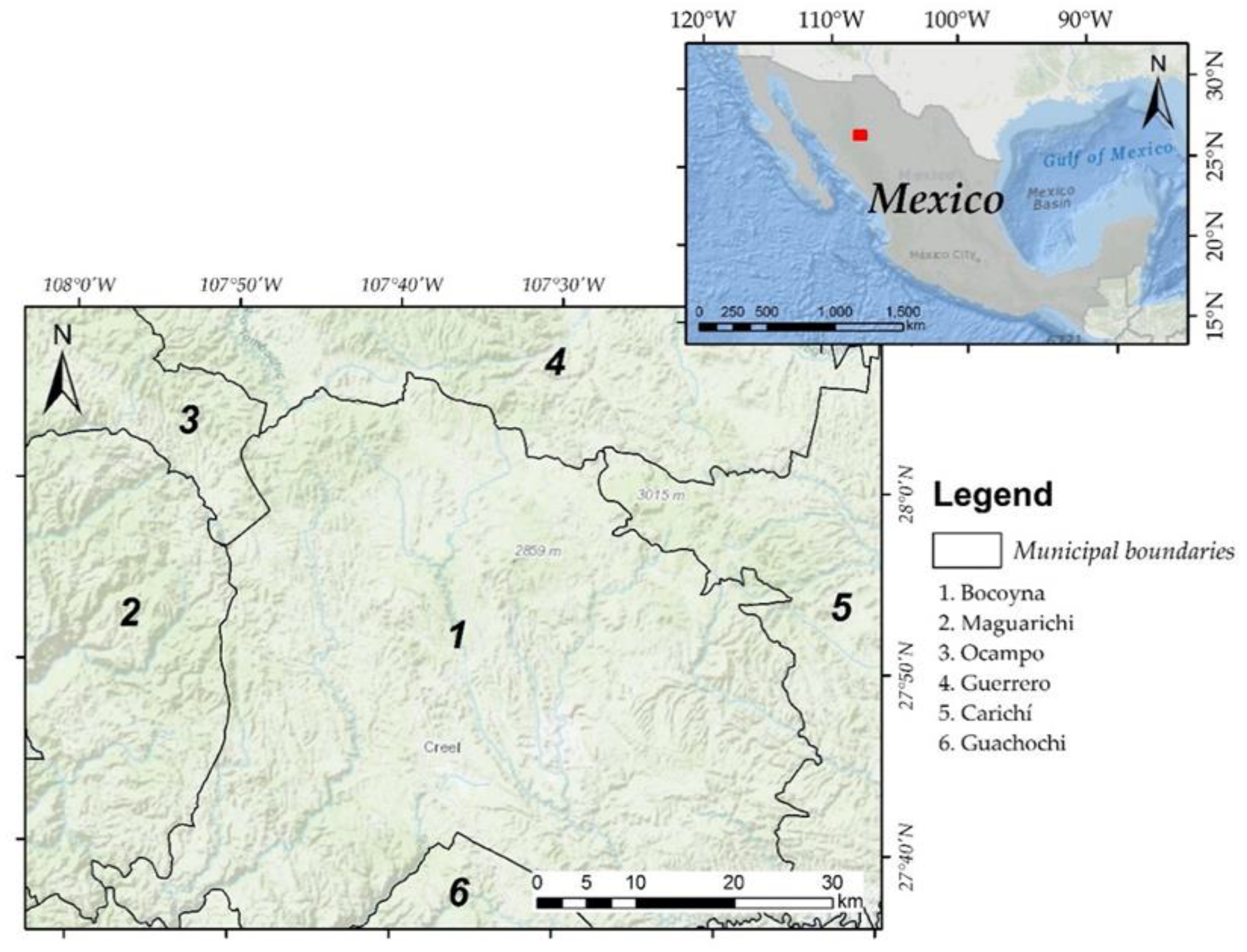
2.1. Study Area
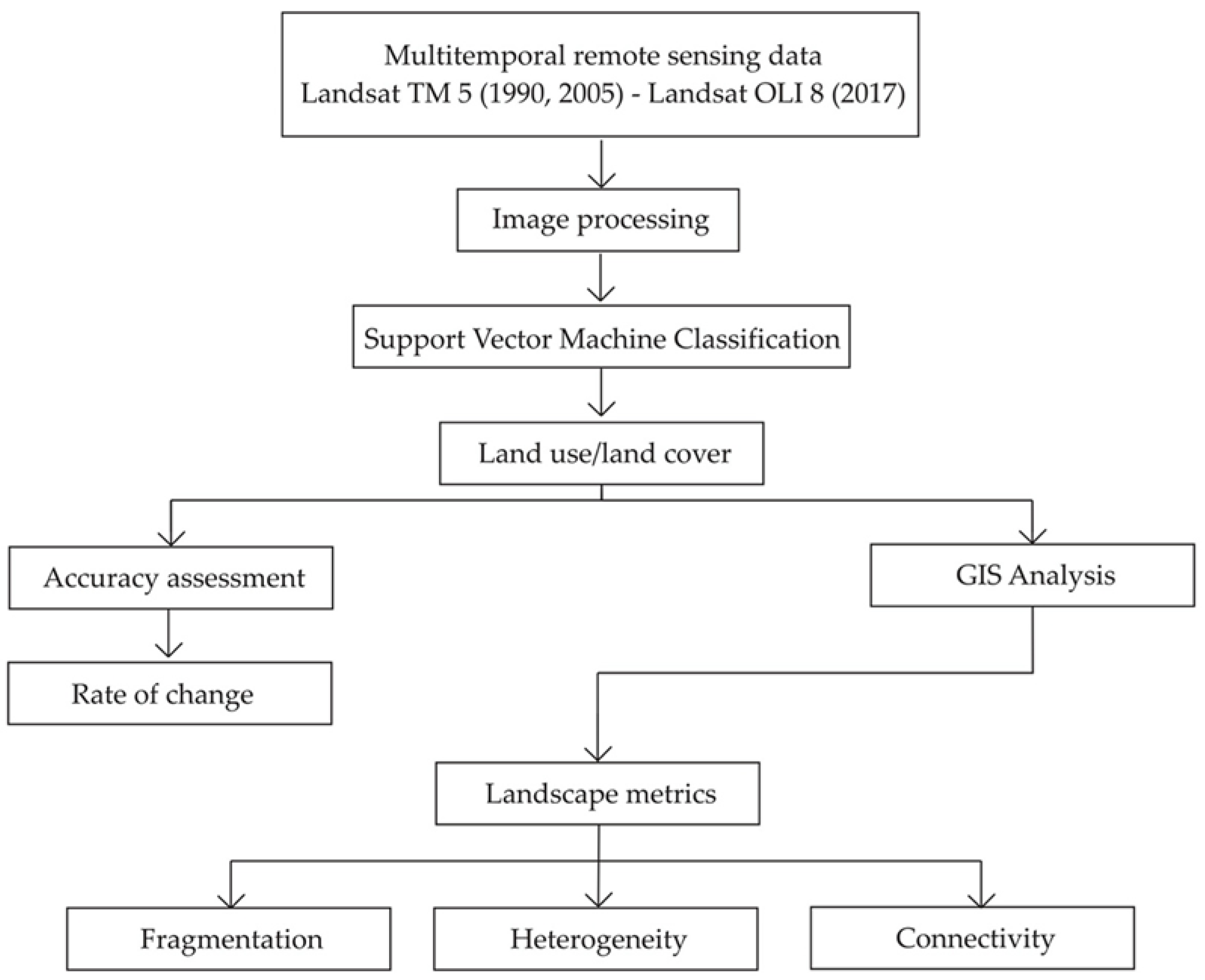
2.2. Framework
2.3. Data Collection
2.4. Data Processing
2.5. Support Vector Machine for Image Classification
2.6. Classification Accuracy
2.7. Conventional Estimation of Areas of Land Use/Land Cover
2.8. Landscape Metrics
3. Results
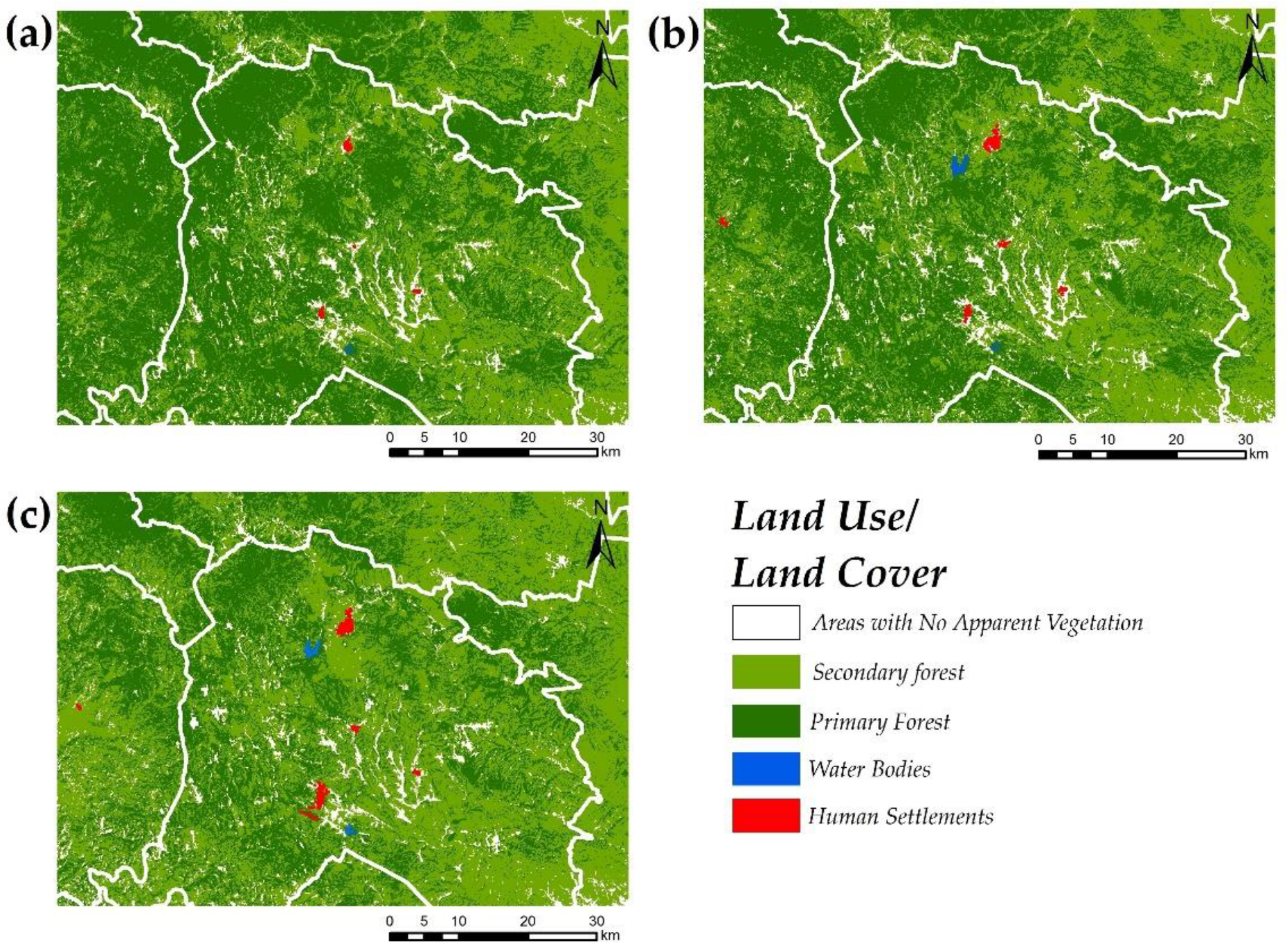
3.1. Land Use/Land Cover Classification of 1990, 2005 and 2017
3.2. Patterns of Land Use/Land Cover Change
3.3. Landscape Metrics Assessment
3.3.1. Metric at the Landscape Level
3.3.2. Metrics at the Class Level
4. Discussion
4.1. Land-Use/Land-Cover Classification
4.2. Metrics at the Landscape and Class Levels
5. Conclusions
Author Contributions
Funding
Acknowledgments
Conflicts of Interest
References
- Shapiro, A.C.; Aguilar-Amuchastegui, N.; Hostert, P.; Bastin, J.F. Using fragmentation to assess degradation of forest edges in Democratic Republic of Congo. Carbon Balance Manag. 2016, 11, 11. [Google Scholar] [CrossRef]
- Zimbres, B.; Peres, C.A.; Machado, R.B. Terrestrial mammal responses to habitat structure and quality of remnant riparian forests in an Amazonian cattle-ranching landscape. Biol. Conserv. 2017, 206, 283–292. [Google Scholar] [CrossRef] [Green Version]
- Barelli, C.; Albanese, D.; Donati, C.; Pindo, M.; Dallago, C.; Rovero, F.; Cavalieri, D.; Tuohy, K.M.; Hauffe, H.C.; De Filippo, C. Habitat fragmentation is associated to gut microbiota diversity of an endangered primate: Implications for conservation. Sci. Rep. 2015, 5, 14862. [Google Scholar] [CrossRef] [Green Version]
- Reddy, C.S.; Manaswini, G.; Satish, K.V.; Singh, S.; Jha, C.S.; Dadhwal, V.K. Conservation priorities of forest ecosystems: Evaluation of deforestation and degradation hotspots using geospatial techniques. Ecol. Eng. 2016, 91, 333–342. [Google Scholar] [CrossRef]
- Cojoc, E.I.; Postolache, C.; Olariu, B.; Beierkuhnlein, C. Effects of anthropogenic fragmentation on primary productivity and soil carbon storage in temperate mountain grasslands. Environ. Monito. Asses. 2016, 188, 653. [Google Scholar] [CrossRef]
- Flores-Rentería, D.; Yuste, J.C.; Rincón, A.; Brearley, F.Q.; García-Gil, J.C.; Valladares, F. Habitat fragmentation can modulate drought effects on the plant-soil-microbial system in Mediterranean holm oak (Quercus ilex) forests. Microb. Ecol. 2015, 69, 798–812. [Google Scholar] [CrossRef] [Green Version]
- Riutta, T.; Clack, H.; Crockatt, M.; Slade, E.M. Landscape-scale implications of the edge effect on soil fauna activity in a temperate forest. Ecosystems 2016, 19, 534–544. [Google Scholar] [CrossRef] [Green Version]
- Schmeller, D.S.; Loyau, A.; Bao, K.; Brack, W.; Chatzinotas, A.; De Vleeschouwer, F.; Friesenh, J.; Gandoisb, L.; Hanssonbi, S.V.; Haverb, M.; et al. People, pollution and pathogens–Global change impacts in mountain freshwater ecosystems. Sci. Total Environ. 2018, 622, 756–763. [Google Scholar] [CrossRef] [Green Version]
- Haila, Y.R.J.O. Islands and Fragments. Maintaining Biodiversity in Forest Ecosystems; Cambridge University Press: Cambridge, UK, 1999; pp. 234–264. [Google Scholar]
- Murcia, C. Edge effects in fragmented forests: Implications for conservation. TREE 1995, 10, 58–62. [Google Scholar] [CrossRef]
- Lanrance, W. Reflections on the tropical deforestation crisis. Biol. Conserv. 1999, 91, 109.e117. [Google Scholar]
- Cayuela, L.; Benayas, J.; Echeverria, C. Clearance and fragmentation of tropical montane forests in the highlands of Chiapas, Mexico (1975 e 2000). For. Ecol. Manag. 2006, 226, 208.e218. [Google Scholar] [CrossRef]
- Auffret, A.G.; Plue, J.; Cousins, S.A. The spatial and temporal components of functional connectivity in fragmented landscapes. Ambio 2015, 44, 51–59. [Google Scholar] [CrossRef] [Green Version]
- Wan, H.; Cushman, S.; Ganey, J. Habitat fragmentation reduces genetic diversity and connectivity of the Mexican spotted owl: A simulation study using empirical resistance models. Genes 2018, 9, 403. [Google Scholar] [CrossRef] [PubMed] [Green Version]
- Brudvig, L.A.; Damschen, E.I.; Haddad, N.M.; Levey, D.J.; Tewksbury, J.J. The influence of habitat fragmentation on multiple plant–animal interactions and plant reproduction. Ecology 2015, 96, 2669–2678. [Google Scholar] [CrossRef] [PubMed]
- Haddad, N.M.; Brudvig, L.A.; Clobert, J.; Davies, K.F.; Gonzalez, A.; Holt, R.D.; Lovejoy, T.E.; Sexton, J.O.; Austin, M.P.; Collins, C.D.; et al. Habitat fragmentation and its lasting impact on Earth’s ecosystems. Sci. Adv. 2015, 1, e1500052. [Google Scholar] [CrossRef] [Green Version]
- Santo-Silva, E.E.; Almeida, W.R.; Tabarelli, M.; Peres, C.A. Habitat fragmentation and the future structure of tree assemblages in a fragmented Atlantic forest landscape. Plant Ecol. 2016, 217, 1129–1140. [Google Scholar] [CrossRef]
- Pardo, L.E.; Campbell, M.J.; Edwards, W.; Clements, G.R.; Laurance, W.F. Terrestrial mammal responses to oil palm dominated landscapes in Colombia. PLoS ONE 2018, 13, e0197539. [Google Scholar] [CrossRef] [Green Version]
- Vallejos, M.; Volante, J.N.; Mosciaro, M.J.; Vale, L.M.; Bustamante, M.L.; Paruelo, J.M. Transformation dynamics of the natural cover in the Dry Chaco ecoregion: A plot level geo-database from 1976 to 2012. J. Arid Environ. 2015, 123, 3–11. [Google Scholar] [CrossRef] [Green Version]
- Carranza, M.L.; Hoyos, L.; Frate, L.; Acosta, A.T.; Cabido, M. Measuring forest fragmentation using multitemporal forest cover maps: Forest loss and spatial pattern analysis in the Gran Chaco, central Argentina. Lands Urban Plann. 2015, 143, 238–247. [Google Scholar] [CrossRef]
- Kumar, R.; Nandy, S.; Agarwal, R.; Kushwaha, S.P.S. Forest cover dynamics analysis and prediction modeling using logistic regression model. Ecol. Indic. 2014, 45, 444–455. [Google Scholar] [CrossRef]
- Chen, D.; Stow, D. The effect of training strategies on supervised classification at different spatial resolutions. Photogramm. Eng. Remote Sensing 2002, 68, 1155–1162. [Google Scholar]
- Healey, S.P.; Cohen, W.B.; Zhiqiang, Y.; Krankina, O.N. Comparison of Tasseled Cap-based Landsat data structures for use in forest disturbance detection. Remote Sens. Environ. 2005, 97, 301–310. [Google Scholar] [CrossRef]
- Wulder, M.A.; White, J.C.; Loveland, T.R.; Woodcock, C.E.; Belward, A.S.; Cohen, W.B.; Fosnight, E.A.; Shaw, J.; Masek, J.G.; Roy, D.P. The global Landsat archive: Status, consolidation, and direction. Remote Sens. Environ. 2016, 185, 271–283. [Google Scholar] [CrossRef] [Green Version]
- Cohen, W.B.; Goward, S.N. Landsat’s Role in Ecological Applications of Remote Sensing. BioScience 2004, 54, 535–545. [Google Scholar] [CrossRef]
- Lizarazo, I.; Elsner, P. Fuzzy segmentation for object-based image classification. Int. J. Remote Sens. 2009, 30, 1643–1649. [Google Scholar] [CrossRef]
- Vapnik, V. The Nature of Statistical Learning Theory; Springer: New York, NY, USA, 1995. [Google Scholar]
- Mantero, P.; Moser, G.; Serpico, S.B. Partially supervised classification of remote sensing images through SVM-based probability density estimation. IEEE Trans. Geosci. Remote Sens. 2005, 43, 559–570. [Google Scholar] [CrossRef]
- Li, M.; Zhu, Z.; Vogelmann, J.E.; Xu, D.; Wen, W.; Liu, A. Characterizing fragmentation of the collective forests in southern China from multitemporal Landsat imagery: A case study from Kecheng district of Zhejiang province. Appl. Geogr. 2011, 31, 1026–1035. [Google Scholar] [CrossRef]
- Turner, M.G.; Gardner, R.H.; O’Neill, R.V. Landscape Ecology in Theory and Practice. Pattern and Process, 2nd ed.; Springer: New York, NY, USA, 2015; pp. 154–196. [Google Scholar]
- McAlpine, C.A.; Eyre, T.J. Testing landscape metrics as indicators of habitat loss and fragmentation in continuous eucalypt forests (Queensland, Australia). Landsc. Ecol. 2002, 17, 711–728. [Google Scholar] [CrossRef]
- Carrara, E.; Arroyo-Rodríguez, V.; Vega-Rivera, J.H.; Schondube, J.E.; de Freitas, S.M.; Fahrig, L. Impact of landscape composition and configuration on forest specialist and generalist bird species in the fragmented Lacandona rainforest, Mexico. Biol. Conserv. 2015, 184, 117–126. [Google Scholar] [CrossRef]
- McGarigal, K.; Tagil, S.; Cushman, S.A. Surface metrics: An alternative to patch metrics for the quantification of landscape structure. Landsc. Ecol. 2009, 24, 433–450. [Google Scholar] [CrossRef]
- Lindenmayer, D.B.; Cunningham, R.B.; Donnelly, C.F.; Leslie, R. On the use of landscape surrogates as ecological indicators in fragmented forests. For. Ecol. Manag. 2002, 159, 203–216. [Google Scholar] [CrossRef]
- Reddy, C.S.; Sreelekshmi, S.; Jha, C.S.; Dadhwal, V.K. National assessment of forest fragmentation in India: Landscape indices as measures of the effects of fragmentation and forest cover change. Ecol. Eng. 2013, 60, 453–464. [Google Scholar] [CrossRef]
- Chuvieco, E. Measuring changes in landscape pattern from satellite images: Short-term effects of fire on spatial diversity. Int. J. Remote Sens. 1999, 20, 2331–2346. [Google Scholar] [CrossRef]
- Leitao, A.B.; Ahern, J. Applying landscape ecological concepts and metrics in sustainable landscape planning. Landsc. Urban Plan. 2002, 59, 65–93. [Google Scholar] [CrossRef]
- CONABIO (Comisión Nacional para el Conocimiento y Uso de la Biodiversidad). Estrategia Nacional Sobre Biodiversidad de México, 1st ed.; Comisión Nacional para el Conocimiento y Uso de la Biodiversidad: Ciudad de México, México, 2001. [Google Scholar]
- Valencia, S. Diversidad del género Quercus (Fagaceae) en México. Boletín de la Sociedad Botánica de México 2004, 75, 33–53. [Google Scholar] [CrossRef] [Green Version]
- Herrera, A. Situación actual de los bosques de Chihuahua. Madera y Bosques 2002, 8, 3–18. [Google Scholar] [CrossRef]
- Prieto-Amparán, J.A.; Villarreal-Guerrero, F.; Martínez-Salvador, M.; Manjarrez-Domínguez, C.; Vázquez-Quintero, G.; Pinedo-Alvarez, A. Spatial near future modeling of land use and land cover changes in the temperate forests of Mexico. PeerJ 2019, 7, e6617. [Google Scholar] [CrossRef] [PubMed] [Green Version]
- CONABIO (Comisión Nacional para el Conocimiento y Uso de la Biodiversidad). La Biodiversidad en Chihuahua: Estudio de Estado, 1st ed.; Comisión Nacional para el Conocimiento y Uso de la Biodiversidad: Ciudad de México, México, 2014; pp. 23–25. [Google Scholar]
- INEGI (Instituto Nacional de Estadística, Geografía e Informática). Síntesis de Información Geográfica del Estado de Chihuahua, 1st ed.; Instituto Nacional de Estadística, Geografía e Informática: Aguascalientes, México, 2003; p. 113. [Google Scholar]
- Gingrich, R.W. The Political Ecology of Deforestation in the Sierra Madre Occidental of Chihuahua. Master’s Thesis, University of Arizona, Tuscon, AZ, USA, 1993. [Google Scholar]
- United States Geological Survey (USGS). GloVis. Available online: http://glovis.usgs.gov (accessed on 13 November 2019).
- Chavez, P.S., Jr. An improved dark-object subtraction technique for atmospheric scattering correction of multispectral data. Remote Sens. Environ. 1988, 24, 459–479. [Google Scholar] [CrossRef]
- Vermote, E.F.; Tanré, D.; Deuze, J.L.; Herman, M.; Morcette, J.J. Second simulation of the satellite signal in the solar spectrum, 6S: An overview. IEEE Trans. Geosci. Remote Sens. 1997, 35, 675–686. [Google Scholar] [CrossRef] [Green Version]
- Hall, F.G.; Strebel, D.E.; Nickeson, J.E.; Goetz, S.J. Radiometric rectification: Toward a common radiometric response among multidate, multisensor images. Remote Sens. Environ. 1991, 35, 11–27. [Google Scholar] [CrossRef]
- Lu, D.; Mausel, P.; Brondizio, E.; Moran, E. Assessment of atmospheric correction methods for Landsat TM data applicable to Amazon basin LBA research. Int. J. Remote Sens. 2002, 23, 2651–2671. [Google Scholar] [CrossRef]
- Congedo, L. Semi-Automatic Classification Plugin for QGIS; Technical Report; Sapienza University, ACC Dar Project: Rome, Italy, 2013. [Google Scholar]
- Kuhn, M. Building predictive models in R using the caret package. J. Stat. Softw. 2008, 28, 1–26. [Google Scholar] [CrossRef] [Green Version]
- Mountrakis, G.; Im, J.; Ogole, C. Support vector machines in remote sensing: A review. ISPRS J. Photogramm. 2011, 66, 247–259. [Google Scholar] [CrossRef]
- Bishop, C.M. Pattern Recognition and Machine Learning, 1st ed.; Springer: Berlin/Heidelberg, Germany, 2006. [Google Scholar]
- Congalton, R.G. Remote sensing and geographic information system data integration: Error sources and research issues. Photogramm. Eng. Remote Sens. 1991, 57, 677–687. [Google Scholar]
- Mas, J.F.; Velázquez, A.; Couturier, S. La evaluación de los cambios de cobertura/uso del suelo en la República Mexicana. Investigación Ambiental Ciencia y Política Pública 2009, 1, 23–39. [Google Scholar]
- Su, S.; Yang, C.; Hu, Y.; Luo, F.; Wang, Y. Progressive landscape fragmentation in relation to cash crop cultivation. Appl. Geogr. 2014, 53, 20–31. [Google Scholar] [CrossRef]
- Remmel, T.K.; Csillag, F. When are two landscape pattern indices significantly different? J. Geogr. Syst. 2003, 5, 331–351. [Google Scholar] [CrossRef]
- Neel, M.C.; McGarigal, K.; Cushman, S.A. Behavior of class-level landscape metrics across gradients of class aggregation and area. Landsc. Ecol. 2004, 19, 435–455. [Google Scholar] [CrossRef]
- Costa, R.L.; Prevedello, J.A.; de Souza, B.G.; Cabral, D.C. Forest transitions in tropical landscapes: A test in the Atlantic Forest biodiversity hotspot. Appl. Geogr. 2017, 82, 93–100. [Google Scholar] [CrossRef]
- Del Castillo, E.M.; García-Martin, A.; Aladrén, L.A.L.; de Luis, M. Evaluation of forest cover change using remote sensing techniques and landscape metrics in Moncayo Natural Park (Spain). Appl. Geogr. 2015, 62, 247–255. [Google Scholar] [CrossRef]
- Tian, Y.; Jim, C.Y.; Tao, Y.; Shi, T. Landscape ecological assessment of green space fragmentation in Hong Kong. Urban For. Urban Green. 2011, 10, 79–86. [Google Scholar] [CrossRef]
- FRAGSTATS Help. Available online: https://www.umass.edu/landeco/research/fragstats/documents/fragstats.help.4.2.pdf (accessed on 16 August 2021).
- Manandhar, R.; Odeh, I.; Ancev, T. Improving the accuracy of land use and land cover classification of Landsat data using post-classification enhancement. Remote Sens. 2009, 1, 330–344. [Google Scholar] [CrossRef] [Green Version]
- Anderson, J.R. A Land Use and Land Cover Classification System for Use with Remote Sensor Data; U.S. Government Printing Office: Washington, DC, USA, 1976.
- Van Vliet, J.; Bregt, A.K.; Hagen-Zanker, A. Revisiting Kappa to account for change in the accuracy assessment of land-use change models. Ecol. Model. 2011, 222, 1367–1375. [Google Scholar] [CrossRef]
- Araya, Y.H.; Cabral, P. Analysis and modeling of urban land cover change in Setúbal and Sesimbra, Portugal. Remote Sens. 2010, 2, 1549–1563. [Google Scholar] [CrossRef] [Green Version]
- Singh, S.K.; Srivastava, P.K.; Gupta, M.; Thakur, J.K.; Mukherjee, S. Appraisal of land use/land cover of mangrove forest ecosystem using support vector machine. Environ. Earth Sci. 2014, 71, 2245–2255. [Google Scholar] [CrossRef]
- Ewers, R.M.; Didham, R.K.; Pearse, W.D.; Lefebvre, V.; Rosa, I.M.D.; Carreiras, J.M.B. Using landscape history to predict biodiversity patterns in fragmented landscapes. Ecol. Lett. 2013, 16, 1221.e1233. [Google Scholar] [CrossRef] [Green Version]
- Gounaridis, D.; Zaimes, G.N.; Koukoulas, S. Quantifying spatio-temporal patterns of forest fragmentation in Hymettus Mountain, Greece. Comput. Environ. Urban Syst. 2014, 46, 35–44. [Google Scholar] [CrossRef]
- Rosa, I.M.; Gabriel, C.; Carreiras, J.M. Spatial and temporal dimensions of landscape fragmentation across the Brazilian Amazon. Reg. Environ. Chang. 2017, 17, 1687–1699. [Google Scholar] [CrossRef] [Green Version]
- Echeverría, C.; Coomes, D.; Salas, J.; Rey-Benayas, J.M.; Lara, A.; Newton, A. Rapid deforestation and fragmentation of Chilean temperate forests. Biol. Conserv. 2006, 130, 481–494. [Google Scholar] [CrossRef]
- Shoyama, K.; Braimoh, A.K. Analyzing about sixty years of land-cover change and associated landscape fragmentation in Shiretoko Peninsula, Northern Japan. Landsc. Urban Plan. 2011, 101, 22–29. [Google Scholar] [CrossRef]
- Fuller, D.O. Forest fragmentation in Loudoun County, Virginia, USA evaluated with multitemporal Landsat imagery. Landsc. Ecol. 2001, 16, 627–642. [Google Scholar] [CrossRef]
- Vazquez, Q.G.; Pinedo, A.A.; Manjarrez, D.C.; De Leon, M.G.; Hernandez, R.A. Analysis of temperate forest fragmentation using spatial medium-resolution remote sensing in Pueblo Nuevo, Durango. Tecnociencia Chihuahua 2013, 7, 88–98. [Google Scholar]
- Cottam, M.R.; Robinson, S.K.; Heske, E.J.; Brawn, J.D.; Rowe, K.C. Use of landscape metrics to predict avian nest survival in a fragmented midwestern forest landscape. Biol. Conserv. 2009, 142, 2464–2475. [Google Scholar] [CrossRef]
- Midha, N.; Mathur, P.K. Assessment of forest fragmentation in the conservation priority Dudhwa landscape, India using FRAGSTATS computed class level metrics. J. Indian Soc. Remote Sens. 2010, 38, 487–500. [Google Scholar] [CrossRef]
- Xue, X.; Hualin, X.; Yuanhua, F. Spatiotemporal Patterns and Drivers of Forest Change from 1985–2000 in the Beijing-Tianjin-Hebei Region of China. J. Resour. Ecol. 2016, 7, 301–308. [Google Scholar] [CrossRef]
- Wen, L.; Luo, Y. Exploring the composition of operation plan for the collective forests in Guizhou province. Sichuan For. Explor. Des. 1996, 2, 36.e38. [Google Scholar]
- Atauri, J.A.; de Lucio, J.V. The role of landscape structure in species richness distribution of birds, amphibians, reptiles and lepidopterans in Mediterranean landscapes. Landsc. Ecol. 2001, 16, 147–159. [Google Scholar] [CrossRef]
- Zhou, X.; Wang, Y.C. Spatial–temporal dynamics of urban green space in response to rapid urbanization and greening policies. Landsc. Urban Plan. 2011, 100, 268–277. [Google Scholar] [CrossRef]
- Tolessa, T.; Senbeta, F.; Kidane, M. Landscape composition and configuration in the central highlands of Ethiopia. Ecol. Evol. 2016, 6, 7409–7421. [Google Scholar] [CrossRef]
- Hartter, J.; Southworth, J. Dwindling resources and fragmentation of landscapes around parks: Wetlands and forest patches around Kibale National Park, Uganda. Landsc. Ecol. 2009, 24, 643. [Google Scholar] [CrossRef]
- Zanella, L.; Borém, R.A.T.; Souza, C.G.; Alves, H.M.R.; Borém, F.M. Atlantic forest fragmentation analysis and landscape restoration management scenarios. Nat. Conserv. 2012, 10, 57–63. [Google Scholar] [CrossRef]
- Costea, G.; Serradj, A.; Haidu, I. Forest cartography using Landsat imagery, for studying deforestation over three catchments from Apuseni mountains, Romania. Adv. Remote Sens. Finite Differ. Inf. Secur. 2012, 109–114. [Google Scholar]
- Peña-Jiménez, A.; Neyra-González, L.; Peña-Jiménez, A.; Neyra-González, L.; Loa-Loza, L.; Durand-Smith, L. Amenazas a la Biodiversidad. La Diversidad Biológica de México: Estudio País; Comisión Nacional Para el Conocimiento y Uso de la Biodiversidad: Ciudad de México, México, 1998; pp. 158–181. [Google Scholar]
- González, B.A. La Sierra Tarahumara, el Bosque y los Pueblos Originarios: Estudio de Caso de Chihuahua México. 2012. Available online: http://www.fao.org/forestry/17194-0381f923a6bc236aa91ecf614d92e12e0.pdf (accessed on 14 November 2019).
- Caballero Deloya, M. La verdadera cosecha maderable en México. Rev. Mex. Cienc. For. 2010, 1, 6–16. [Google Scholar]
- Pérez-Verdín, G.; Márquez-Linares, M.A.; Cortés-Ortiz, A.; Salmerón-Macías, M. Análisis espacio-temporal de la ocurrencia de incendios forestales en Durango, México. Madera y Bosques 2013, 19, 37–58. [Google Scholar] [CrossRef]


| Sensor | Capture Date | Characteristics |
|---|---|---|
| Landsat TM 5 | 1990 | 6 spectral bands with a spatial resolution of 30 m, 1 thermal band with a spatial resolution of 120 m |
| Landsat TM 5 | 2005 | 6 spectral bands with a spatial resolution of 30 m, 1 thermal band with a spatial resolution of 120 m |
| Landsat OLI 8 | 2017 | 8 spectral bands with a spatial resolution of 30 m, 1 panchromatic band with a resolution of 15 m, 2 thermal bands with a resolution of 100 m |
| Landscape Metrics | Description | Level of Analysis | Unit | Type |
|---|---|---|---|---|
| Number of Patches (NumP) | Number of patches of the corresponding patch type | L/C | # | Fragmentation |
| Patch Density (PD) | Number of patches of the corresponding patch type divided by total landscape area. | L/C | # of patches/100 ha | Fragmentation |
| Edge Density (ED) | Sum of the lengths (m) of all edge segments involving the corresponding patch type, divided by the total landscape area (m2), multiplied by 10,000 (to convert to hectares). | L | m ha−1 | Fragmentation |
| Mean Patch Size (MPS) | Sum of the areas (m2) of all patches of the corresponding patch type, divided by the number of patches of the same type, divided by 10,000 (to convert to hectares) | L/C | ha | Fragmentation |
| Perimeter-Area Fractal Dimension (PAFRAC) | Equals 2 divided by the slope of regression line obtained by regressing the logarithm of patch area (m2) against the logarithm of patch perimeter (m). | L | Unitless | Fragmentation |
| Shannon’s Diversity Index (SHDI) | Equals minus the sum, across all patch types, of the proportional abundance of each patch type multiplied by that proportion | L | Unitless | Heterogeneity |
| Percentage of Landscape (PLAND) | Quantifies the proportional abundance of each patch type in the landscape, as a fundamental measure of landscape composition (only at the class level) | C | % | Fragmentation |
| Euclidean Nearest Neighbor Distance (ENN_MN) | Distance (m) to the nearest neighboring patch of the same type, based on shortest edge-to-edge distance. | C | m | Connectivity |
| Patch Cohesion Index (COHESION) | Equals 1 minus the sum of patch perimeter (in terms of number of cell surfaces) divided by the sum of patch perimeter times the square root of patch area (in terms of number of cells) for patches of the corresponding patch type, divided by 1 minus 1 over the square root of the total number of cells in the landscape, multiplied by 100 to convert to a percentage. | C | Unitless | Connectivity |
| Land Use/Land Cover | 1990 | 2005 | 2017 |
|---|---|---|---|
| Areas with No Apparent Vegetation | 0.80 | 0.84 | 0.83 |
| Secondary Forest | 0.78 | 0.72 | 0.73 |
| Human Settlements | 0.84 | 0.88 | 0.87 |
| Water Bodies | 1.00 | 1.00 | 1.00 |
| Primary Forest | 0.77 | 0.81 | 0.80 |
| Overall KAPPA | 0.84 | 0.85 | 0.85 |
| Land Use/Land Cover | Occupied Area (ha) | Change Rate (% y−1) | ||||
|---|---|---|---|---|---|---|
| 1990 | 2005 | 2017 | 1990–2005 | 2005–2017 | 1990–2017 | |
| Areas with no apparent vegetation | 20,444.18 | 23,828.59 | 24,101.92 | 0.89 | 0.14 | 0.94 |
| Secondary forest | 19,9121.38 | 22,3948.16 | 28,6922.04 | 0.87 | 3.37 | 0.97 |
| Human settlements | 154.60 | 272.35 | 521.65 | 0.98 | 10.98 | 1.03 |
| Water bodies | 26.97 | 103.76 | 153.91 | 1.07 | 5.80 | 1.06 |
| Primary forest | 27,7380.46 | 248,973.97 | 185,427.79 | −0.86 | −3.06 | −0.96 |
| Year | NumP (#) | PD (# of Patches/100 ha) | ED (m ha−1) | MPS (ha) | PAFRAC | SHDI |
|---|---|---|---|---|---|---|
| 1990 | 19,905.00 | 4.00 | 70.72 | 20.695 | 1.54 | 0.83 |
| 2005 | 22,619.00 | 4.55 | 76.81 | 18.269 | 1.51 | 0.86 |
| 2017 | 22,115.00 | 4.45 | 79.86 | 18.618 | 1.53 | 0.84 |
| PD (# of Patches/100 ha) | PLAND (%) | ENN_MN (m) | |||||||
| 1990 | 2005 | 2017 | 1990 | 2005 | 2017 | 1990 | 2005 | 2017 | |
| AWV | 8.54 | 10.16 | 11.30 | 4.12 | 4.84 | 57.68 | 245.16 | 229.88 | 89.74 |
| SF | 59.99 | 65.23 | 67.95 | 40.09 | 45.06 | 37.32 | 105.24 | 94.53 | 103.28 |
| HS | 0.04 | 0.14 | 0.17 | 0.03 | 0.05 | 4.86 | 11,845.33 | 108.52 | 214.82 |
| WB | 0.01 | 0.05 | 0.03 | 0.01 | 0.02 | 0.11 | N/A | 2022.44 | 1325 |
| PF | 53.51 | 57.44 | 58.46 | 55.75 | 50.03 | 0.03 | 99.41 | 100.62 | 25,153 |
| MPS (ha) | NumP (#) | COHESION | |||||||
| 1990 | 2005 | 2017 | 1990 | 2005 | 2017 | 1990 | 2005 | 2017 | |
| AWV | 5.24 | 5.03 | 4.32 | 3905.00 | 4734.00 | 5577.00 | 95.12 | 95.15 | 93.85 |
| SF | 15.28 | 16.42 | 32.75 | 13,035.00 | 13,638.00 | 8761.00 | 99.83 | 99.83 | 99.95 |
| HS | 25.77 | 1.99 | 12.13 | 6.00 | 137.00 | 43.00 | 95.63 | 94.27 | 96.49 |
| WB | 26.97 | 4.94 | 76.96 | 1.00 | 21.00 | 2.00 | 94.25 | 95.46 | 96.85 |
| PF | 39.21 | 28.68 | 15.05 | 7075.00 | 8682.00 | 12,318.00 | 99.95 | 99.93 | 99.65 |
Publisher’s Note: MDPI stays neutral with regard to jurisdictional claims in published maps and institutional affiliations. |
© 2021 by the authors. Licensee MDPI, Basel, Switzerland. This article is an open access article distributed under the terms and conditions of the Creative Commons Attribution (CC BY) license (https://creativecommons.org/licenses/by/4.0/).
Share and Cite
Legarreta-Miranda, C.K.; Prieto-Amparán, J.A.; Villarreal-Guerrero, F.; Morales-Nieto, C.R.; Pinedo-Alvarez, A. Long-Term Land-Use/Land-Cover Change Increased the Landscape Heterogeneity of a Fragmented Temperate Forest in Mexico. Forests 2021, 12, 1099. https://doi.org/10.3390/f12081099
Legarreta-Miranda CK, Prieto-Amparán JA, Villarreal-Guerrero F, Morales-Nieto CR, Pinedo-Alvarez A. Long-Term Land-Use/Land-Cover Change Increased the Landscape Heterogeneity of a Fragmented Temperate Forest in Mexico. Forests. 2021; 12(8):1099. https://doi.org/10.3390/f12081099
Chicago/Turabian StyleLegarreta-Miranda, Claudia K., Jesús A. Prieto-Amparán, Federico Villarreal-Guerrero, Carlos R. Morales-Nieto, and Alfredo Pinedo-Alvarez. 2021. "Long-Term Land-Use/Land-Cover Change Increased the Landscape Heterogeneity of a Fragmented Temperate Forest in Mexico" Forests 12, no. 8: 1099. https://doi.org/10.3390/f12081099
APA StyleLegarreta-Miranda, C. K., Prieto-Amparán, J. A., Villarreal-Guerrero, F., Morales-Nieto, C. R., & Pinedo-Alvarez, A. (2021). Long-Term Land-Use/Land-Cover Change Increased the Landscape Heterogeneity of a Fragmented Temperate Forest in Mexico. Forests, 12(8), 1099. https://doi.org/10.3390/f12081099