Abstract
Elevated acid deposition has been a concern in the central Appalachian region for decades. A long-term acidification experiment on the Fernow Experimental Forest in central West Virginia was initiated in 1996 and continues to this day. Ammonium sulfate was used to simulate elevated acid deposition. A concurrent lime treatment with an ammonium sulfate treatment was also implemented to assess the ameliorative effects of base cations to offset acidification. We show that the forest vegetation simulator growth model can be locally calibrated and used to project stand growth and development over 40 years to assess the impacts of acid deposition and liming. Modeled projections showed that pin cherry (initially) and sweet birch responded positively to nitrogen and sulfur additions, while black cherry, red maple, and cucumbertree responded positively to nitrogen, sulfur, and lime. Yellow-poplar negatively responded to both treatments. Despite these differences, our projections show a maximum of 5% difference in total stand volume among treatments after 40 years.
1. Introduction
The influence of acid rain on the health and productivity of forest ecosystems has been a topic of research interest since the late-1970s to early-1980s [1,2,3]. High concentrations of coal fired power plants in the Ohio River Valley have historically been a major source of nitrous oxides (NOx) and sulfur oxides (SOx), which are released into the atmosphere [4]. These gases are released from the combustion of fossil fuels and once in the atmosphere, both gases have a high affinity for water vapor and quickly form the most common forms of acid rain: nitric (HNO3) and sulfuric (H2SO4) acids [5]. Due to the relatively short mean residence time of water in the atmosphere, these acids are deposited in higher quantities in the form of acidic precipitation across the mid-Atlantic and northeastern United States [6].
When nitric and sulfuric acids are deposited into forested areas in the Central Appalachian region, they have both direct and indirect negative influences on the associated forest soils. A large percentage of the soils of the central Appalachian hardwood forest region are at risk for base cation depletion from soil acidification and nitrogen saturation [7]. These soils are normally low in base cations such as calcium (Ca2+) and magnesium (Mg2+), which also limits their buffering capacity [8]. As H2SO4 and HNO3 deposition increases, hydrogen ions (H+) disassociate in soil solution, which increases the rates of mineral weathering and displaces cations from cation exchange sites [9,10]. Additionally, H+ ions associate with aluminum (Al3+) bearing compounds, increasing the amount of aluminum ions in soil solution, which negatively affects root growth [11,12]. Aluminum ions have a high affinity for cation exchange sites and displace plant essential cations such as Ca2+ and Mg2+ [11,12]. If not taken up by plants rather quickly, calcium and magnesium ions are leached from the soil, further decreasing soil fertility [4]. Increased Al3+ concentrations in soil can also reduce the rate of nitrate (NO3−) uptake by trees, allowing increased NO3− leaching from soils [13].
A secondary process associated with the deposition of nitric acid is nitrogen saturation. When inputs of nitrogen from atmospheric deposition, mineralization, and atmospheric sequestration become greater than the need of the organisms in the system, an ecosystem can be considered N saturated [14]. Excess nitrate is leached from the soil due to the low capacity of central Appalachian forests to retain nitrate [15]. As systems reach nitrogen saturation, the nitrification of ammonium (NH4+) to nitrate increases, leading to additional losses of N from the system [16]. Other negative effects of increased N include lower soil pH values [16,17,18], reduced base cation uptake due to Al3+ mobilization [18,19,20], and increased release of greenhouse gas emissions from soils [21,22].
The response of forests to inputs of chronic N and sulfur (S) are dependent on location and duration of the inputs. The Fork Mountain Long-Term Soil Productivity site (LTSP) was established within the U.S. Forest Service Fernow Experimental Forest (FEF) in 1996 as part of a nationwide effort to quantify the basic controls on forest soil productivity [23]. One of the goals of the Fork Mountain LTSP study was to characterize the effects of acid deposition on newly regenerating central Appalachian forest vegetation. The acid deposition was simulated by annual N + S additions at rates mimicking deposition at the time. Additionally, an ameliorative treatment in which lime was added to balance the N + S additions was also evaluated.
Research on this site and others within the FEF have highlighted some of the immediate impacts of increased nitrogen on forest vegetation. For example, commercially important species such as yellow-poplar (Liriodendron tulipifera L.) show decreased incremental growth after seven years of nitrogen and sulfur inputs [24]. Similarly, biomass accumulation by sweet birch (Betula lenta L.) and yellow-poplar decreased in areas with increased chronic N inputs [24]. Fowler et al. [25] concurrently observed a decrease in tree species diversity associated with elevated rates of N and S. However, the total plant biomass of a forest community can be stimulated by sustained increases in nitrogen inputs [26,27,28]. The extent and duration of these responses are variable and species-specific, but eventually, the negative effects of soil acidification are theorized to outweigh the positive effect of increased nitrogen availability [29].
Unfortunately, the long-term effects of elevated acidic deposition on forest growth have been studied to a lesser extent, mainly due to the lack of long-term/rotation length data [30]. As such, growth and yield models can offer the opportunity to examine these impacts on time scales outside the available data. The goal of our paper was to demonstrate that the Forest Vegetation Simulator (FVS), which is a distance-independent, single-tree growth model [31], can be calibrated to central Appalachian forests and used to model the impacts of elevated acidic inputs over time. FVS is a widely used growth simulator for addressing forest changes over time due to natural succession, management and natural disturbances, and proposed management. The regional variant (NE) of FVS covers the northeast region from West Virginia to Maine, which gives it broad applicability to modeling growth and stand development. However, since the model covers such a large region, model estimates tend to vary considerably, and out-of-the-box performance is often undesirable [32]. Many have noted the need to calibrate FVS in order to achieve more accurate simulations (e.g., [33,34]).
Although other studies have used FVS for similar goals (e.g., [30]), our application to the LTSP study provides a unique opportunity to model long-term stand growth for an Appalachian hardwood stand that was exposed to these conditions for over 20 years beginning at its inception, rather than modeling existing stands or simulating regeneration. This study utilizes data from the LTSP study to compare the effects of elevated acidic deposition and an ameliorative liming treatment on stand growth.
2. Materials and Methods
Data used for this study were derived from stands located in the USDA Forest Service Fernow Experimental Forest (FEF) near Parsons, West Virginia (latitude 39°04′ N, longitude 79°41′ W). The 1862-ha forest has been utilized as a research and teaching forest by the USFS since its establishment in 1934. Over this time period, key topics of long-term research have included silvicultural management for the production of high-quality hardwoods, the effects of harvesting on water quality, and ecosystem responses to acidic deposition.
The Fork Mountain Long-term Soil Productivity (LTSP) site is approximately 12.1 ha with a predominant southeast aspect and slopes between 15 and 30 percent, and the elevation ranges from approximately 792 to 853 m a.s.l. At the initiation of the study, the stand was 85 years old, and the site index (base age 50) for red oak was 24.3 m. The most prevalent species across the study site included northern red oak (Quercus rubra L.), sugar maple (Acer saccharum Marsh.), black cherry (Prunus serotina Ehrh.), and yellow-poplar, which comprised over 70% of the stand basal area. The soils on site are Calvin and Berks (Loamy-skeletal, mixed, active, mesic Typic Dystrudepts) and Hazelton series (Loamy-skeletal, siliceous, active, mesic Typic Dystrudepts) and are derived from sandstone colluvium, sandstone residuum, and weathered shale. Soils are well drained and loamy with the typical soil chemical characteristics for the region (Appendix A, Table A1). More specific details concerning the site and vegetation characteristics can be found in Adams et al. [35].
In the LTSP, the effects of elevated rates of acidic deposition on forest productivity were examined using four treatments replicated four times across the site. The treatments included an uncut control (CTRL), whole tree harvest (WT), whole tree harvest with the addition of ammonium sulfate fertilizer (WT + NS), and whole tree harvest + ammonium sulfate fertilizer + dolomitic lime (WT + NS + LIME). However, for the purposes of this study, we only considered the harvested plots (WT, WT + NS, and WT + NS + LIME treatments). Each treatment plot encompassed 0.4047 ha. The ammonium sulfate was added at twice the ambient nitrogen (15.0 kg N/ha/yr) and sulfur (17.0 kg S/ha/yr) deposition rates [35]. The dolomitic lime was added at twice the rate of calcium (11.2 kg Ca/ha/yr) and magnesium (5.8 kg Mg/ha/yr) export from a watershed in close proximity to the site [36]. The ammonium sulfate and dolomitic lime have been applied during March, July, and November each year since the site was harvested. The dolomitic lime addition was designed to mitigate the negative effects of soil acidification in order to better understand the effect of continual nitrogen addition on the ecosystem.
Data were collected across the study site using a total of 60 randomly selected subplots (five per treatment plot on each of the 12 treatment and block replicates) that were sampled in 2017 (age 21). Each subplot consisted of two nested circular measurement plots. Trees between 2.5–12.7 cm dbh were measured on 0.004 ha (3.59 m radius) plots, while trees greater than 12.7 cm dbh were measured on 0.04 ha (11.35 m radius) plots. Total height was measured using a clinometer on select dominant and codominant trees of the most common species on site. The number of height measurements varied by species, depending on the availability of codominant and dominant stems within the plots.
2.1. Growth Projections
Growth of the three treatments was projected using the northeast variant of FVS [37]. Datasets from 18 plots in nine calibration stands located across the FEF were used to modify the model to local conditions. These stands were all regenerated using an even age seed tree regeneration method, with initial harvest occurring between August 1960 and August 1962 [38]. Initial harvests removed most of the trees, with the remaining trees removed within three years after the initial harvest. The landscape features varied among sites (Table 1), but generally the plots ranged between 610–915 m a.s.l. in elevation. The soils are typically characterized as moderately deep, well drained residuum that were formed from the weathering of shale, sandstone, or siltstone. The Belmont series is the one exception, which was derived from mainly limestone (USDA, n.d.) and was retained to provide the range of species and stand conditions needed to calibrate the model.

Table 1.
Description of site features and age 20 stand parameters associated with the 18 calibration plots used for model calibration.
Each calibration stand was quantified using two permanent 0.10 ha plots (18 total) that have been periodically measured by U.S. Forest Service personnel since the stands were approximately 20 years of age. All trees greater than 2.5 cm dbh were tagged and dbh measurements were recorded for each tree.
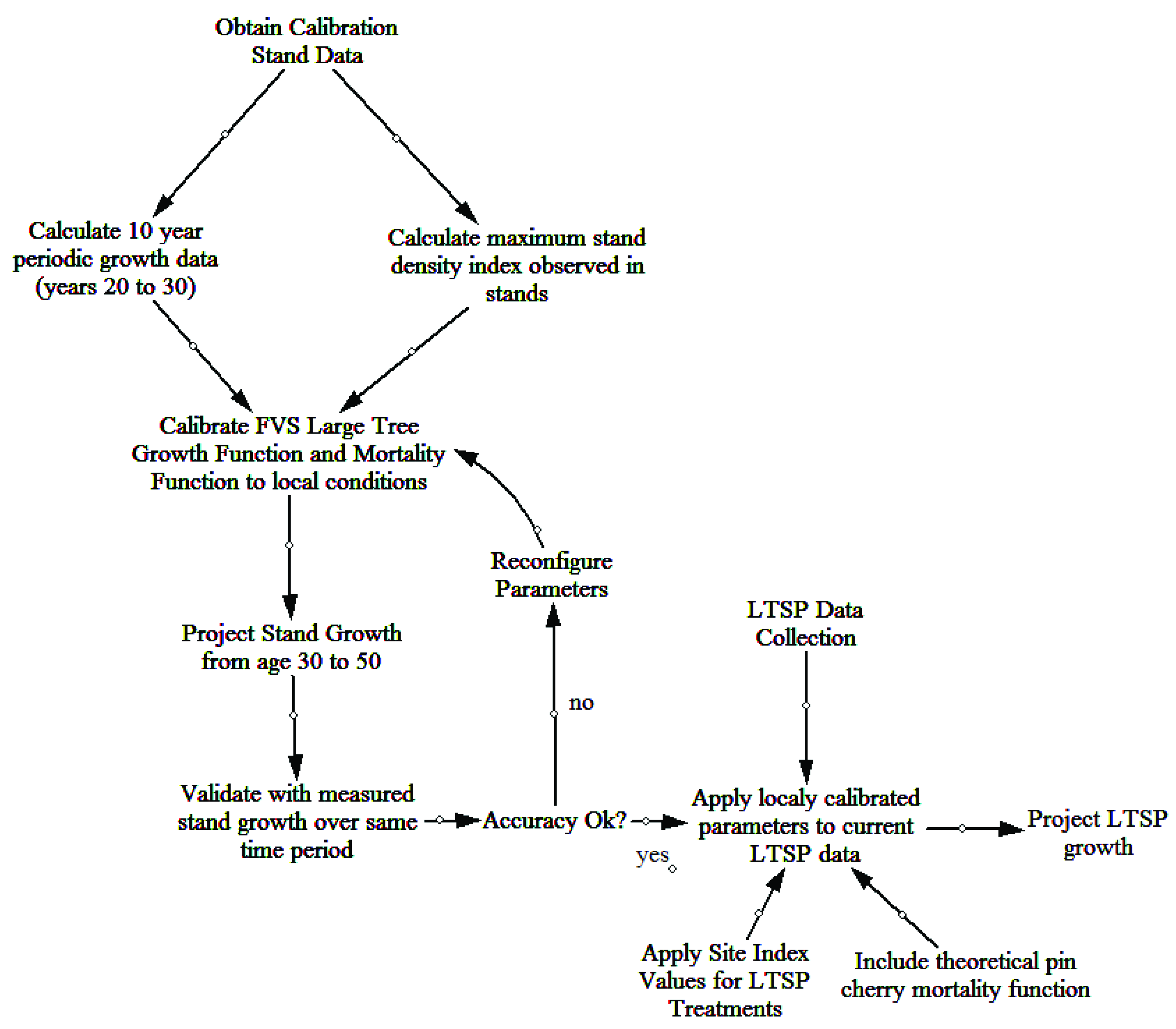
Thirty years of individual tree data from the 18 permanent plots on the FEF were used to calibrate FVS to local growing conditions. Initially, the base model performance was tested against this dataset to determine what, if any, modifications were necessary. Trees per ha (TPH) and basal area (m2/ha) were used as the metrics for comparison between actual and predicted values. The evaluation of non-calibrated model projections indicated poor out-of-box performance. The two parameters of greatest concern within the model were the mortality and large tree basal area growth (trees ≥ 12.7 cm dbh). A workflow for the calibration and validation of the FVS NE model to local growing conditions of the FEF is provided (Figure 1).
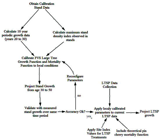
Figure 1.
Workflow for calibration and validation of the northeast variant of the forest vegetation simulator for the Fernow Experimental Forest.
Mortality was adjusted in the FVS based on a maximum stand density index (SDI) value. Maximum stand density index was based off calculated SDI values using the data available from the calibration stands across all time periods (ages 20–50). Within the calibration stands, the maximum observed SDI value was 786 and was used for all future model simulations. The default percentages of 55% and 85% for initiating density-dependent mortality and stand maximum density, respectively, were retained [37].
The growth data from the first 10 years of periodic measurements were used to calibrate the large tree basal area growth. Each live tree (at age 30) was assigned a 10 year incremental growth value, equivalent to the observed growth from age 20–30. The “Growth” keyword was used to read the data into the model and project the growth of individuals based on observed values. The “CalbStat” keyword was used to calculate the growth of each species relative to the base model predicted growth. The model was based on a one year time step and growth modifications that were applied during every time step in the projection.
To account for differences in growth on the treatments of the LTSP plots, treatment specific site index values were included in the model. Yellow-poplar was chosen as the species for this adjustment due to its high abundance and large number of dominant and codominant stems in the stand. Site index values were estimated from site index curves for the Appalachian mountain region [38]. Site index (base age 50 years) values for the three treatments areas were calculated as 35.1 m for WT plots and 33.5 m for WT + NS and WT + NS + LIME plots. There was a consistent trend of higher site index values for the WT plots in comparison to the WT + NS and WT + NS + LIME for most species. The projections for the WT + NS and WT + NS + LIME plots assumed that the response to the treatments would remain constant across all time periods of the model projection.
A second scenario (continual decline scenario) was included in the model for the WT + NS and WT + NS + LIME treatments to describe a continued negative response of the overstory to nitrogen and sulfur inputs. On average, yellow-poplar trees in fertilized plots grew about 1.5 m less in total height (after 20 years) compared to non-fertilized trees. If this negative trend were to occur for the remainder of the projection period, the site index at the end of the projection period (age 60 years) would be reduced to 32.9 m for the fertilized treatments [39].
One final adjustment made to the final model was to account for the natural dynamics of pin cherry (Prunus pensylvanica L. f.). There were very few pin cherries present on the calibration plots by the time the measurements began, so it was not reasonable to think that the model would be able to predict the loss of pin cherry from the site based solely on the calibration data. A theoretical mortality function was included that would generally follow the dynamics described by [40]. In the LTSP study, pin cherry dominance had already begun to senesce based on severely declining relative importance values in 2012 and 2017 [41]. Pin cherry tree mortality was modified in the model by removing 50% of each tree record for each time step until the species was no longer present in the overstory. Mortality was initially concentrated on smaller trees and secondarily on the larger trees. This instruction to the model assumes that the smaller pin cherry trees were less competitive for light resources and therefore die sooner than the larger trees that are receiving full light [42].
2.2. Model Validation
Model validation protocol generally follows the framework developed by the USFS FVS Steering Team [43]. Variables predicted by the base model (ba/ha, TPH, quadratic mean diameter) were first verified by comparing general stand dynamic patterns. Base model performance was analyzed using mean percent error (MPE), root mean squared error (RMSE), and graphical representations of basal area and trees per ha changes over time. Locally calibrated values for maximum SDI and large tree basal area growth were included in the model. The observed vs. predicted TPH and ba/ha values for each calibration stand were again analyzed using MPE, RMSE, and graphs. Once prediction error was reduced to less than 15% MPE for both TPH and ba/ha [44], the modified model parameters were applied to the LTSP plot data.
3. Results
3.1. Model Calibration
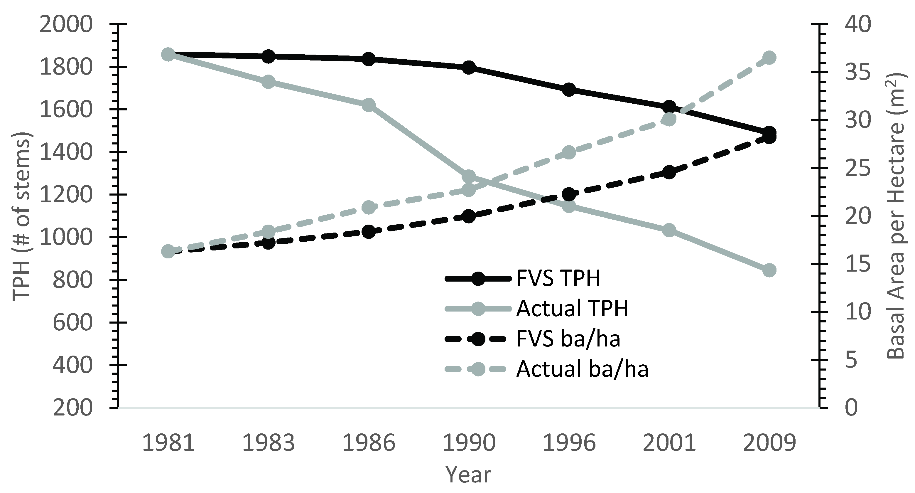
Overall, the base model (uncalibrated) performed poorly for TPH and basal area. Uncalibrated FVS consistently predicted higher TPH and lower basal area per ha values relative to field measurements (Figure 2). Across all stands and measurement periods, FVS over-predicted TPA values by approximately 33%, with a maximum over-prediction of 90%. The mean percent error of TPH at the end of the 30 year projection period was 59% greater than measurements in the nine calibration stands. Average basal area projections were approximately 19% lower on average than the observed values for all stands and time periods.
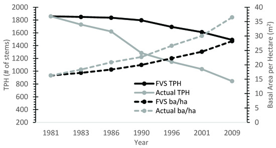
Figure 2.
Base FVS model performance plotted against actual growth data for calibration stand 32. Model bias was consistent across all calibration stands.
Results from the large tree basal area growth calibration revealed several species growing at higher rates on the FEF compared to base model predictions. Increased growth rates were calculated for the following species: red maple (Acer rubrum L.) (13.2%), sweet birch (41.8%), yellow-poplar (14.2%), black cherry (21.5%), chestnut oak (Quercus montana Willd.) (10.3%), and slippery elm (Ulmus rubra Muhl.) (4.8%) (Appendix A, Table A2). For each species, the large tree basal area growth parameter was modified by a multiplier to increase growth at every time step.
3.2. Model Validation
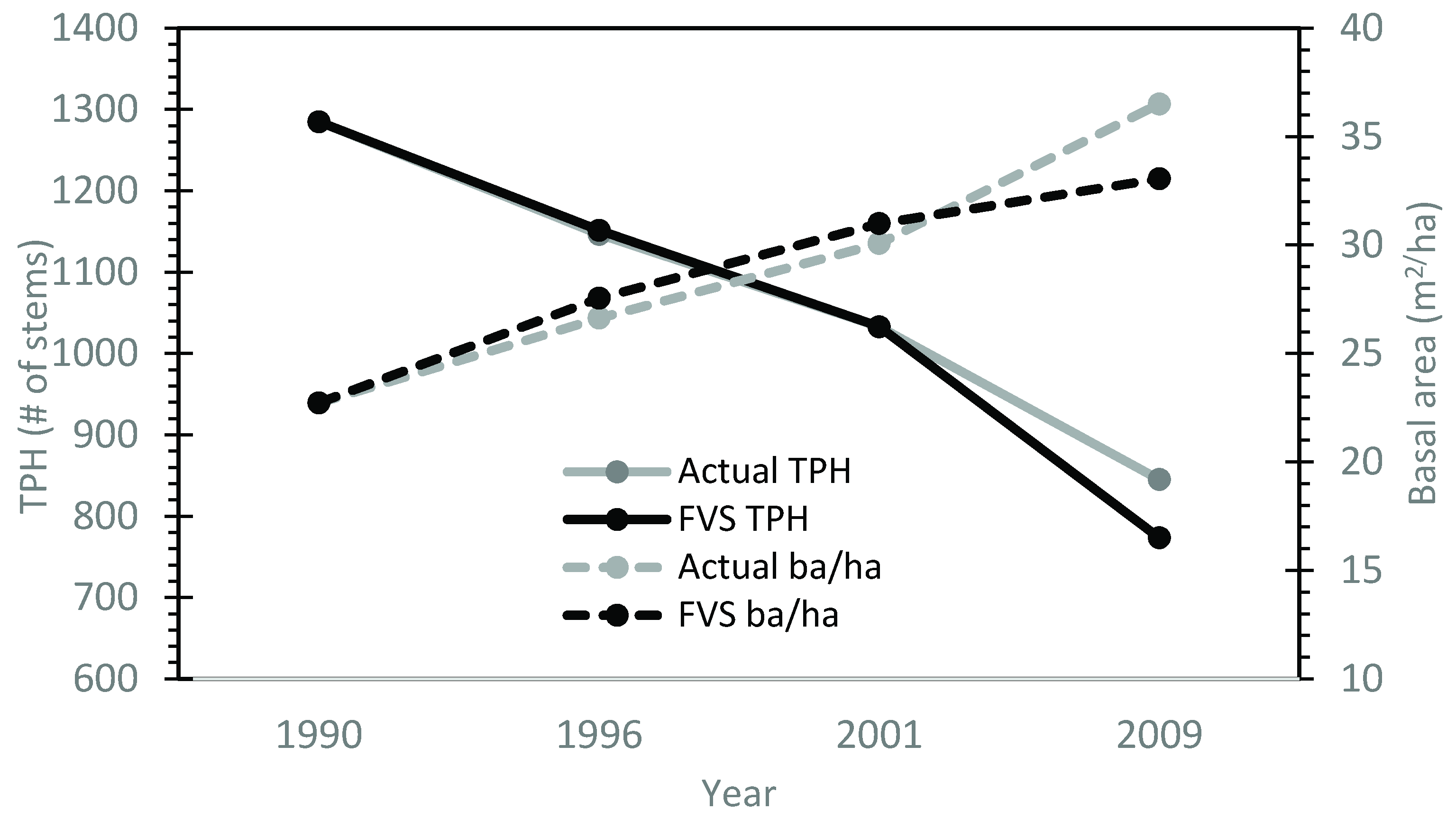
After the calibration of the max SDI and large tree basal area growth functions, the model was applied to the calibration stand data for year 30 and growth was predicted over the next 20 years. The predicted values for trees/ha and basal area/ha were similar to the observed values. On average, the calibrated model reduced the systematic error in base model performance by 71% for MPE of TPH and 81% for MPE of ba/ha (Table 2). Average root mean square error values for TPH averaged 106 trees/ha for all stands. Average trees per ha MPE for all stands was ±7.7%. Basal area per ha RMSE values had an averaged value of approximately 1.8 m2/ha. The overall average MPE for basal area per ha predictions was 3.5%. Generally, deviations from the observed values increased as the model progressed through time (Figure 3).
Table 2.
Mean percent error (MPE) and root mean square error (RMSE) values for trees per hectare and basal area per hectare (m2/ha) calculated by comparing the FVS NE base model and FEF locally calibrated model predictions to the observed values in nine calibration stands. Positive numbers represent an overestimation by the model and negative numbers represent underestimation.
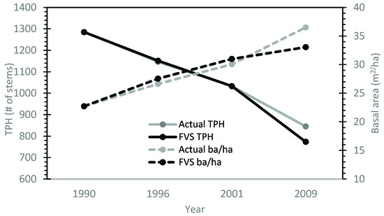
Figure 3.
A visual representation of decreased model systematic error using the locally calibrated FVS model for calibration stand 32 (compared to Figure 1).
3.3. Projection of LTSP Data
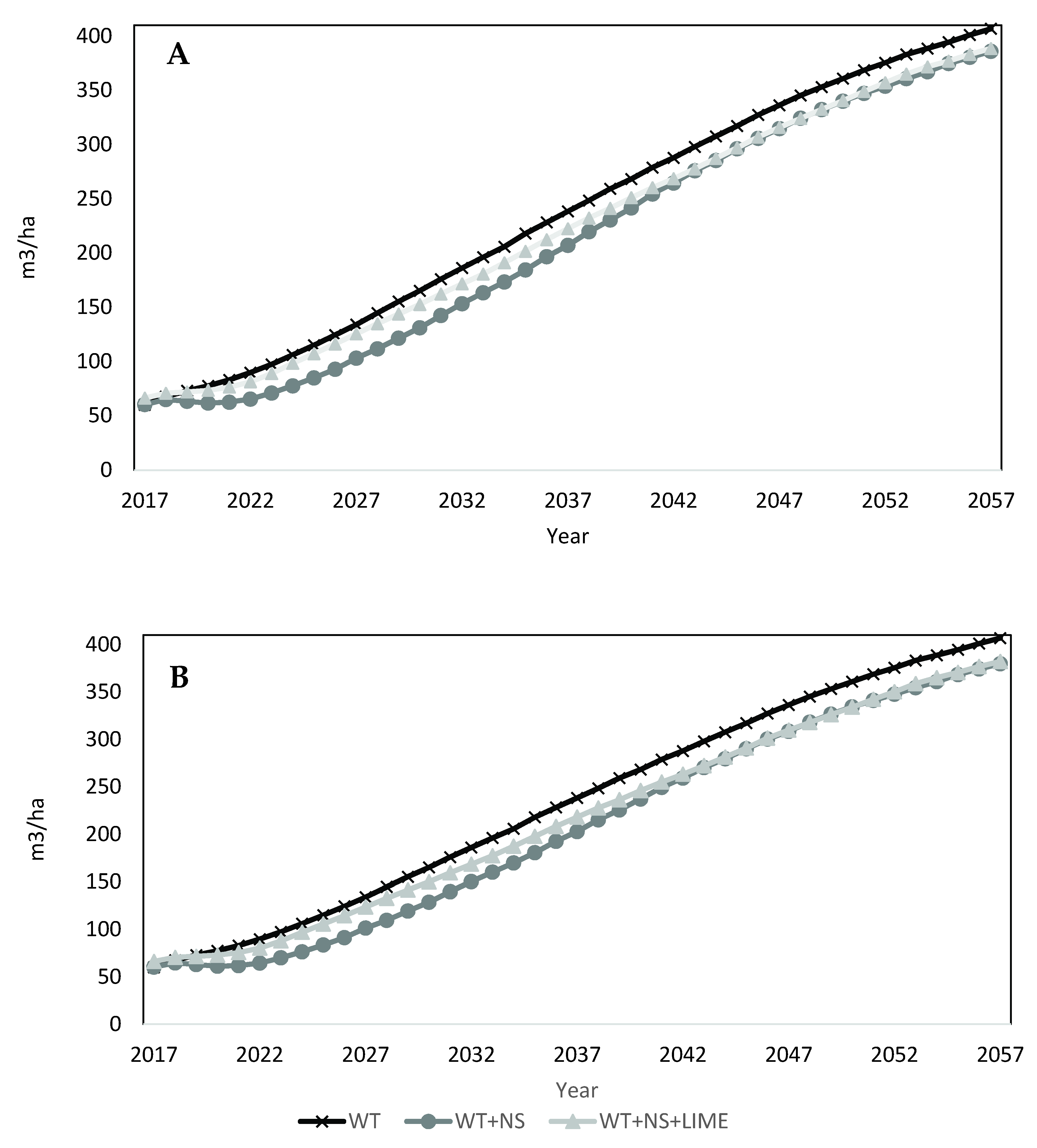
The FEF calibrated model was applied to the year 21 LTSP plot data to project volumes for each treatment over 40 years. Projections indicated an initial, small decrease in volume on site for all treatments (Figure 4A). This response was due to the mortality of pin cherry as it continues its natural life cycle (Figure 5A). The reduction in total volume was less for the WT plots, which had less initial volume of pin cherry present (Table 3). As the projection continues, there is little variation in the total merchantable volume produced among treatments. Volumes at the end of the 40 year projection (61 year-old stands) for WT plots was greatest (407 m3/ha), followed by the WT + NS + LIME plots (389 m3/ha) and the WT + NS plots (386 m3/ha).
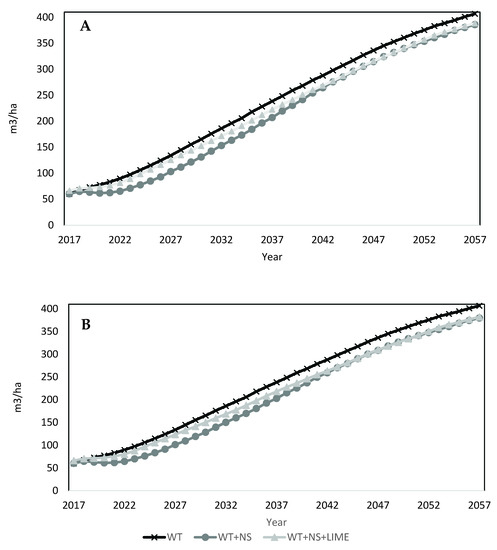
Figure 4.
FVS projections for merchantable volume for all species combined by treatment. (A) Upper graph represents constant decline scenario. (B) Lower graph represents continual decline scenario.
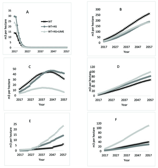
Figure 5.
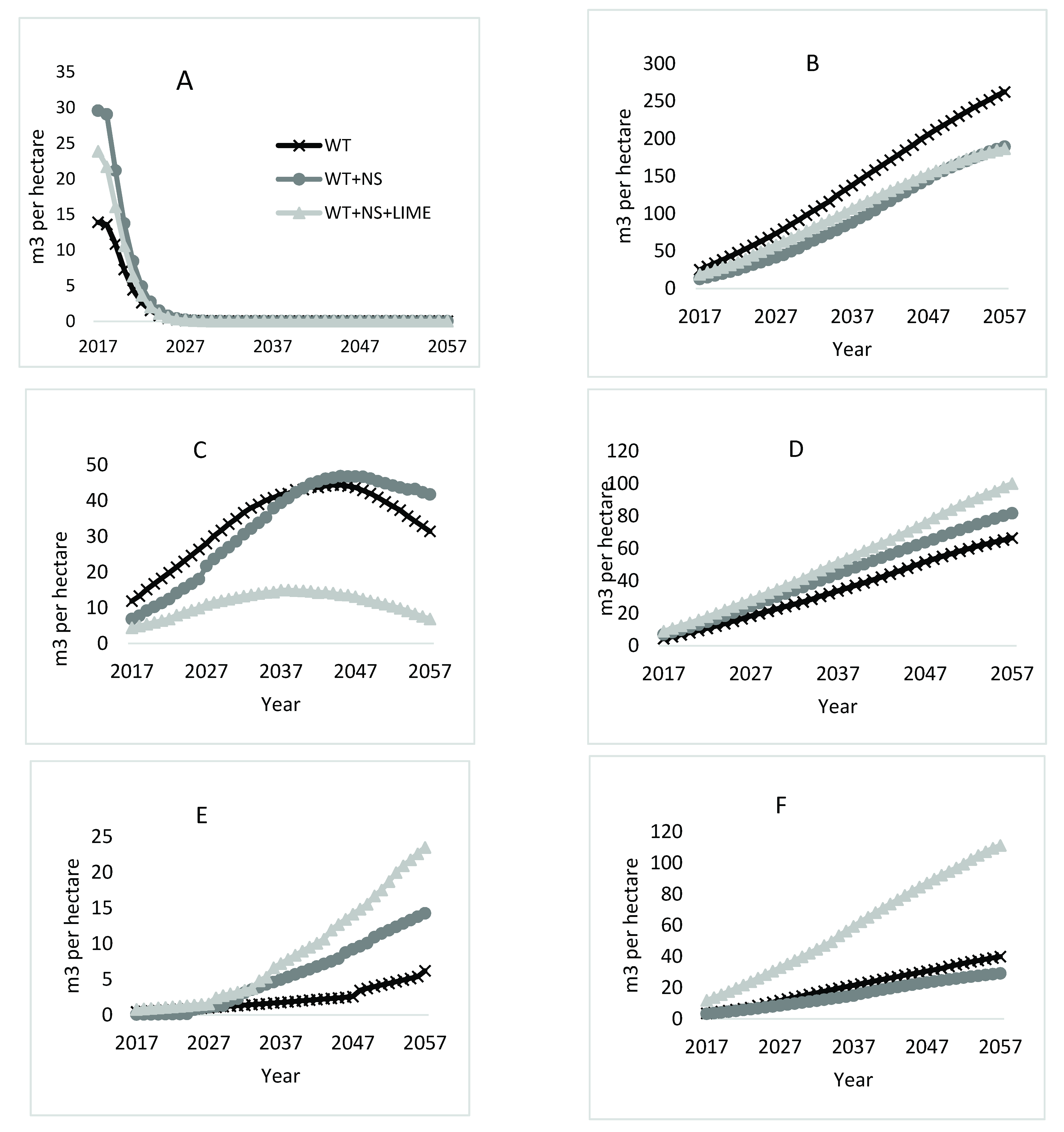
Species specific cumulative growth predictions for three treatments on the LTSP site. Six species (in order of highest lowest importance value at year 2017) (Storm, 2018) are presented by species: (A) pin cherry, (B) yellow-poplar, (C) sweet birch, (D) black cherry, (E) red maple, (F) cucumbertree.
Table 3.
FVS predicted stocking of mean percentage of total trees per ha for the six main species in each treatment area for 10 year projection intervals. Data for all species are included in Appendix A, Table A3.
For the continual decline scenario (Figure 4B), the fertilized treatments resulted in negligible differences by the end of the projection. Final volumes projected for the WT + NS and WT + NS + LIME plots were 380 m3/ha and 382 m3/ha, respectively. For both the declining and fixed impact projection scenarios, their respective WT + NS and WT + NS + LIME treatments had nearly identical volume estimates over time. Therefore, no further results for the continual decline scenarios are provided.
Yellow-poplar was projected to be the dominant species on the site throughout the next 40 years in terms of merchantable volume (Figure 5B) and is the driving species behind the slightly higher total volume in the WT treatment areas. By the end of the projection period, yellow-poplar made up almost 65% of the total volume on the WT plots and approximately 50% on both the WT + NS and WT + NS + LIME plots. At the start of the projection, yellow-poplar stems made up 38% of the trees on WT plots, but only 25% on the WT + NS plots and 21% on the WT + NS + LIME plots (Table 3). The greatest differences in TPH among treatments were for the smallest diameter class (Table 4). For example, yellow-poplar stems in the 5 cm diameter class were nearly three times more abundant on the WT plots than the WT + NS and WT + NS + LIME plots.
Table 4.
Trees per hectare for the top six species by diameter class for the Fork Mountain LTSP in 2017. Data for all species are included in Appendix A, Table A4.
Final volume differences by treatment for black cherry correspond with an initial higher percent trees per ha in the WT + NS + LIME treatment (Table 3). Initially, black cherry stems were nearly three times more abundant on WT + NS + LIME plots than on the WT and WT + NS plots. In addition, there were no black cherry trees on the WT plots greater than the 20 cm diameter class (Table 4). By the end of the projection, black cherry merchantable volume for the WT + NS + LIME treatment was 34 m3/ha more than the WT and 18 m3/ha higher than the WT + NS (Figure 5D).
The growth of cucumbertree over time is projected to also follow a similar linear trend as black cherry and yellow-poplar. At the start of the projections, there was no difference in the initial percent of the total trees per ha in any of the treatment areas for cucumbertree (Table 3). However, there were a greater number of large individual trees that were measured on the WT + NS + LIME plots compared to trees growing in the WT and WT + NS plots (Table 4), which may indicate a positive response of this species to the WT + NS + LIME treatment during the first 21 years. The initial merchantable volume present on WT + NS + LIME plots was over three times greater than that on the other two treatments (Figure 5F). After 40 years of growth, cucumbertree is predicted to account for 100 m3/ha on the WT + NS + LIME plots, 40 m3/ha on the WT plots, and 29 m3/ha on the WT + NS plots.
Red maple projections deviated from the generally linear growth trends for yellow-poplar, black cherry, and cucumbertree. Initially, there were few red maple stems in the WT plots that were greater than 5 cm, which was not the case for the WT + NS and WT + NS + LIME plots (Table 4). Red maple stems were projected to represent little merchantable volume for the first decade of the projections in all treatments (Figure 5E). Around age 33 (year 2029), red maple stems receiving additional nitrogen from the treatments are expected to begin producing merchantable volume, culminating in 24 m3/ha on WT + NS + LIME plots and 14 m3/ha on the WT + NS plots. The volume for red maple stems on WT plots was projected to be lower, only producing 6 m3/ha by age 61 (year 2057).
The total volume of sweet birch is projected to increase for all treatments until the trees are 40–50 (years 2037–2047) years old, after which mortality occurs in all treatments (Figure 5C). The WT + NS + LIME plots that started out with the lowest volume of sweet birch, also reached the point of maximum volume earliest. Between the years 2038 and 2057 in the projection, the volume of sweet birch on WT + NS + LIME plots declined from 15 m3/ha to 7 m3/ha. Both the WT and WT + NS plots reached their respective highest points of merchantable volume between the ages of 47 and 48, respectively. The WT plots reached a maximum predicted value of 44 m3/ha and the WT + NS plots culminated at 47 m3/ha. After this point, the mortality induced reduction in sweet birch volume on the WT plots was projected to decrease at a rate 2.5 times faster than the trees on the WT + NS plots.
4. Discussion
The overall volume growth on the site is not projected to decline substantially over the 40-year projection for any treatment (Figure 4A). However, it does seem that there will be differences in the species that make up the final volume in the treatment areas (Table 3). This shift in species composition could have both economic and environmental implications in the future.
The 40-year volume projections followed patterns that were mostly consistent with trends observed during the first 21 years of treatment [41]. Yellow-poplar, black cherry, red maple, and cucumbertree all showed stable, long-term positive responses to treatments. With the exceptions of yellow-poplar and sweet birch, the other species had the most volume on WT + NS treated areas. For yellow-poplar, plots that received annual nitrogen and sulfur additions were projected to grow less merchantable volume than the WT (non-fertilized) areas. Sweet birch was the only species where the response to treatments changed over time. For the first 20 years of the projections, volume was highest on WT treatments, but after 20 years (41 years of treatment), volume associated with the WT+NS treatments was greatest, and then declined (Figure 5C).
As with all growth models, projections are sensitive to initial stand conditions. For example, projections for black cherry and red maple showed the greatest volume accumulation for the WT + NS + LIME treatments, while yellow-poplar volume accumulation was greatest for WT. All of these responses were associated with the treatments that also had the greatest stem densities at the beginning of the modelling period (stand age 21). However, there are indications that the acidification and liming treatments are responsible for at least some changes in stand growth and development.
In the case of yellow-poplar, which is projected to be the dominant merchantable species in all treatment areas (Figure 5B), the increased volume associated with the WT plots was at least partly attributable to higher numbers of trees per ha in 2017 (21 years-old), and possibly a reflection of early treatment impacts (Table 4). However, considering that yellow-poplar is a shade-intolerant species [45], many of these smaller stems will die as the stand continues to grow over time, which might reduce the long-term impact of the high stem counts in the smallest diameter classes (Table 3). Additionally, there appears to be an ameliorative effect of adding lime to the acidification treatment for yellow-poplar given that the total volume for WT + NS and WT + NS + LIME treatments was similar, even though the number of stems on the liming treatment were much fewer. Despite these apparent effects, the difference between treatments is marked and suggests that the acidification treatment (WT + NS) still results in reduced growth rather than just a function of starting conditions.
Growth and mortality of sweet birch on WT + NS plots differed relative to WT and WT + NS + LIME. Initially, there were fewer stems in all diameter classes on the WT + NS compared to those sampled on WT plots (Table 4), so this response cannot be attributed to additional stems present in the larger diameter classes. It is likely that the model allocated more growing space to sweet birch in the WT + NS treated areas where yellow-poplar was projected to have less volume and because of the loss of pin cherry to mortality. Since mortality in the model is based on the stand density index at any given point in time, there was less mortality assigned to sweet birch stems on the WT + NS plots compared to WT plots later in the projection due to lower number of yellow-poplar stems in the WT + NS plots.
By the end of the projection, red maple made up an increasingly larger percentage of trees in the treatment areas (Table 3). However, red maple only accounted for a small percent of total volume, suggesting that many of the red maple stems will persist in the midstory. This pattern of red maple growth dynamics is well documented [46,47]. The results suggest that chronic additions of nitrogen in the soil (either from deposition or fertilization) could lead to further increases in red maple dominance in eastern hardwood forests, which is a trend that has been noted for the last few decades [48].
The number of black cherry stems at the start of the projections was greater on the WT + NS + LIME plots (Table 4), which was also reflected in high initial stem counts shortly after the stand was regenerated in 1996 [35]. As a result, the increased volume associated with the liming treatment is difficult to separate from the impacts of having much greater stem counts in the initial stand. Additionally, although FVS predicted increased volume on the WT + NS + LIME plots, there is little evidence in the literature to support that liming increases black cherry growth. Liming studies with mature black cherry trees have shown both short- and long-term negative responses to single high rate applications (although different from the annual, low rate applications here) of dolomitic lime in areas of high historic acidic deposition [49,50]. However, young black cherry trees have been shown to increase growth and foliar nutrient concentrations after nitrogen and phosphorus fertilizer [51,52]. In the LTSP study, it seems that black cherry responded positively to the first 21 years of the ammonium sulfate fertilizer (regardless of whether dolomitic lime was added) in terms of growing larger diameter individuals (Table 4) and increased final volume estimations for both WT + NS and WT + NS + LIME treatments compared to the nonfertilized areas.
Certainly, modeling results are always subject to the inherent complexity and accuracy. Our calibration efforts significantly improved the overall model performance. The site indices for the model (YP base age 50: 35.1 m for WT plots, 30.5 m for WT + NS, and WT + NS + LIME; 32.9 m for the continual declining WT + NS and WT + NS + LIME) represent a negative response in growth from the chronic additions of N. This response is corroborated with other reports of decreased growth of yellow-poplar from chronic additions of N on the FEF [24], but does not necessarily represent the response of all species to the treatments. Since height measurements were not collected for all stems and species, the model is limited in predicting individual species response to the additions of ammonium sulfate and lime. Another limitation relates to mortality functions within FVS. Mortality is a function of tree diameter and species specific parameters [37]. The impact of treatments is not directly factored into the model, although indirectly, if a treatment negatively affects diameter growth, the mortality rate is higher. In contrast, some hardwood growth models also factor in relative size [53], so mortality is increased if a tree’s relative size lags behind other stems and species.
Finally, there is a possibility that the impact of the WT + NS and N + S + LIME treatments are either inducing or exacerbating other nutrient deficiencies. There is evidence that high N enrichment, through deposition or fertilization, leads to phosphorus limitations on stand level productivity or for individual species [54,55,56]. Highlighting this possibility, Gress et al. [57] used root ingrowth cores and phosphatase activity in the current study area and nearby watersheds on the FEF to demonstrate a likely phosphorus deficiency and increased root growth for a prominent understory herbaceous plant, Viola rotundifolia, in areas associated with elevated soil, foliar, and stream nitrogen levels. Elevated nitrogen deposition can decrease species richness in certain plant communities [58,59,60] including forests. Whether tree species richness will decline in these central Appalachian hardwood forests because of long-term acid deposition is unknown, but our results showed only modest changes over time that do not appear specific to a particular treatment.
5. Conclusions
The goals of this paper were to provide a framework and calibration metrics for using FVS to model the impacts of acid deposition as well as supplemental liming on the growth of a central WV Appalachian hardwood stand. We showed that significant improvements (>70% improvement in error) to the base model FVS can be achieved to calibrate a locally specific model to project 40 years of additional growth and development of a forest subjected to 20+ years of experimentally elevated nitrogen, sulfur, and lime inputs. Additionally, we showed that species had different growth patterns as a result of the initial and long-term influence of acidification and liming treatments.
Over time, the dominant pin cherry will be eliminated from the stand and the more long-lived species will attain dominance. Although there does appear to be treatment impacts on growth and stand development, pinpointing the casual mechanisms (i.e., inherent stand variability vs. initial treatment effects vs. longer term treatment impacts) is challenging at this point. Likewise, continued N and S inputs may further (or begin to) alter tree growth and stand development into the future. Continued monitoring of this long-term LTSP experiment will allow us to examine the mechanisms responsible for the declining growth of the plots receiving annual nitrogen and sulfur inputs.
Author Contributions
Conceptualization, M.B.A.; Methodology, M.B.A. and J.S.; Formal analysis, A.S.; Writing—original draft preparation, A.S.; Writing—review and editing, J.S. and M.B.A.; Supervision, J.S.; Project administration, J.S. and M.B.A.; Funding acquisition, M.B.A. All authors have read and agreed to the published version of the manuscript.
Funding
This research was funded by the United States Forest Service, Northern Research Station, Timber and Watershed Lab under Joint Venture Agreement Number 15JV11242303102. This material is based upon work that is supported by the National Institute of Food and Agriculture, U.S. Department of Agriculture, McIntire Stennis project WVA00804.
Institutional Review Board Statement
Not applicable.
Informed Consent Statement
Not applicable.
Data Availability Statement
Data analyzed for this study are archived by the United States Forest Service, Northern Research Station, Timber and Watershed Lab, Parsons, WV.
Acknowledgments
The authors express their gratitude to John Juracko and Brian Simpson from the USFS for their assistance in collecting the field data.
Conflicts of Interest
The authors declare no conflict of interest.
Appendix A
Table A1.
Soil chemical characteristics by soil depth at the initiation of the LTSP study (from Adams et al. 2004).
Table A1.
Soil chemical characteristics by soil depth at the initiation of the LTSP study (from Adams et al. 2004).
| Variable | 025 cm | 1530 cm | 3045 cm |
|---|---|---|---|
| % C | 6.58 | 2.71 | 1.12 |
| pH | 4.24 | 4.45 | 4.42 |
| Total N (%) | 0.42 | 0.22 | 0.14 |
| Ca (cmol + /kg) | 0.54 | 0.17 | 0.13 |
| Mg (cmol + /kg) | 0.18 | 0.07 | 0.04 |
| K (cmol + /kg) | 0.33 | 0.34 | 0.12 |
| Al (cmol + /kg) | 3.52 | 3.43 | 3.92 |
| Exch. acidity (cmol + /kg) | 5.3 | 4.12 | 4.68 |
| Total acidity (cmol + /kg) | 27.65 | 18.51 | 13.25 |
| Cation Exch. Capacity (cmol + /kg) | 28.7 | 19.09 | 13.55 |
| % Base Sat. | 3.67 | 2.99 | 1.61 |
Table A2.
Species growing at higher rates in calibration plots than what is normally predicted by FVS NE. Species multiplier values here were used to modify the large tree basal area growth function. Species codes are as follows: RM (red maple), SB (sweet birch), YP (yellow-poplar), BC (black cherry), CO (chestnut oak), SE (slippery elm).
| Scale Factor Summary | |||||||
|---|---|---|---|---|---|---|---|
| SPECIES | N | Min | Mean | Max | Std. Dev. | Total Tree Records | Multiplier |
| RM | 5 | 1.004 | 1.105 | 1.267 | 0.110 | 244 | 1.132 |
| SB | 7 | 1.160 | 1.383 | 1.893 | 0.241 | 164 | 1.418 |
| YP | 6 | 0.669 | 1.160 | 1.543 | 0.330 | 125 | 1.142 |
| BC | 5 | 0.996 | 1.345 | 1.975 | 0.420 | 138 | 1.215 |
| CO | 2 | 1.007 | 1.183 | 1.358 | 0.248 | 67 | 1.103 |
| SE | 2 | 0.816 | 1.008 | 1.200 | 0.272 | 31 | 1.048 |
N = Number of stands that contributed scale factors; MIN = minimum initial scale factor encountered; Mean = mean initial scale factor; MAX = maximum scale factor encountered; Std. dev. = standard deviation for scale factors; Total tree records = total number of trees used to calculate scale factors; Multiplier = mean multiplier to be used to scale the growth of large trees.
Table A3.
FVS predicted stocking of mean percentage of total trees per ha in each treatment area for 10 year projection intervals. Values of 0% represent less than 1% total trees per ha while dashes () represent species absence from the corresponding area.
Table A3.
FVS predicted stocking of mean percentage of total trees per ha in each treatment area for 10 year projection intervals. Values of 0% represent less than 1% total trees per ha while dashes () represent species absence from the corresponding area.
| WT | WT + NS | WT + NS + LIME | |||||||||||||
|---|---|---|---|---|---|---|---|---|---|---|---|---|---|---|---|
| Species * | 2017 | 2027 | 2037 | 2047 | 2057 | 2017 | 2027 | 2037 | 2047 | 2057 | 2017 | 2027 | 2037 | 2047 | 2057 |
| black cherry | 5% | 6% | 6% | 7% | 8% | 5% | 6% | 6% | 7% | 9% | 14% | 17% | 17% | 16% | 16% |
| black locust | 0% | 0% | 0% | 0% | 0% | 1% | 1% | 0% | 0% | ||||||
| cucumbertree | 3% | 3% | 4% | 4% | 5% | 3% | 4% | 3% | 3% | 4% | 3% | 3% | 4% | 6% | 8% |
| eastern hemlock | 0% | 0% | 0% | 0% | 0% | ||||||||||
| hickory spp. | 0% | 0% | 1% | 1% | 1% | 0% | 0% | 0% | 0% | 0% | 1% | 2% | 2% | 1% | 1% |
| Fraser magnolia | 1% | 1% | 1% | 2% | 2% | 4% | 6% | 7% | 8% | 9% | 2% | 3% | 2% | 2% | 2% |
| noncommercial | 3% | 3% | 2% | 1% | 0% | 2% | 2% | 2% | 1% | 0% | |||||
| pin cherry | 11% | 0% | 20% | 0% | 16% | 0% | |||||||||
| red maple | 7% | 9% | 12% | 16% | 20% | 6% | 8% | 10% | 12% | 15% | 12% | 16% | 17% | 22% | 25% |
| red oak | 2% | 2% | 2% | 2% | 2% | 3% | 3% | 2% | 2% | 2% | 3% | 4% | 4% | 4% | 4% |
| sweet birch | 26% | 28% | 25% | 17% | 10% | 24% | 30% | 28% | 23% | 17% | 11% | 13% | 11% | 7% | 2% |
| Sourwood | 2% | 2% | 3% | 4% | 5% | ||||||||||
| Serviceberry | 3% | 4% | 4% | 4% | 2% | 2% | 2% | 2% | 1% | 0% | |||||
| sugar maple | 3% | 4% | 4% | 5% | 6% | ||||||||||
| Sassafras | 1% | 1% | 1% | 0% | 0% | 1% | 2% | 2% | 2% | 1% | |||||
| striped maple | 5% | 7% | 9% | 12% | 13% | 1% | 1% | 2% | 2% | 2% | 6% | 7% | 9% | 11% | 12% |
| white ash | 1% | 1% | 1% | 0% | 0% | 1% | 1% | 1% | 0% | 0% | |||||
| yellow-poplar | 38% | 41% | 38% | 39% | 39% | 25% | 31% | 31% | 31% | 33% | 21% | 24% | 23% | 24% | 24% |
* black cherry (Prunus serotina Ehrh.); black locust (Robinia pseudoacacia L.); cucumbertree (Magnolia acuminata L.); eastern hemlock (Tsuga canadensis (L.) Carr.); hickory spp. (Carya spp.); Fraser magnolia (Magnolia fraseri Walt.); pin cherry (Prunus pensylvanica L. f.); red maple (Acer rubrum L.); red oak (Quercus rubra L.); sweet birch (Betula lenta L.); sourwood (Oxydendrum arboretum (L.) DC.); serviceberry (Amelanchier arborea (Michx. F.) Fernald); sugar maple (Acer saccharum Marsh.); sassafras (Sassafras albidum (Nutt.) Nees); striped maple (Acer pensylvanicum L.); white ash (Fraxinus americana L.); yellow-poplar (Liriodendron tulipifera L.).
Table A4.
Trees per hectare for each species and diameter class for the Fork Mountain LTSP in year 2017.
Table A4.
Trees per hectare for each species and diameter class for the Fork Mountain LTSP in year 2017.
| WT | WT + NS | LIME | ||||||||||||||
|---|---|---|---|---|---|---|---|---|---|---|---|---|---|---|---|---|
| Diameter Class | ||||||||||||||||
| Species | 5 | 10 | 15 | 20 | 25 | 5 | 10 | 15 | 20 | 25 | 5 | 10 | 15 | 20 | 25 | 30 |
| black cherry | 74 | 37 | 37 | 7 | 62 | 12 | 23 | 22 | 4 | 259 | 62 | 27 | 17 | 4 | 5 | |
| black locust | 2 | 12 | 4 | |||||||||||||
| cucumbertree | 49 | 25 | 6 | 9 | 0 | 49 | 12 | 4 | 4 | 2 | 25 | 12 | 14 | 14 | 5 | |
| eastern hemlock | 1 | |||||||||||||||
| hickory | 12 | 1 | 25 | 12 | ||||||||||||
| Fraser magnolia | 12 | 10 | 4 | 62 | 37 | 7 | 12 | 25 | 16 | 9 | ||||||
| noncommercial | 49 | 25 | 62 | |||||||||||||
| pin cherry | 62 | 124 | 148 | 30 | 2 | 62 | 148 | 222 | 65 | 11 | 37 | 161 | 170 | 56 | 9 | |
| red maple | 198 | 12 | 4 | 86 | 62 | 1 | 235 | 86 | 4 | 1 | ||||||
| red oak | 62 | 49 | 1 | 1 | 49 | 37 | 4 | |||||||||
| sweet birch | 556 | 185 | 88 | 19 | 371 | 148 | 65 | 7 | 148 | 111 | 36 | 7 | ||||
| sourwood | 12 | 25 | 2 | |||||||||||||
| serviceberry | 74 | 49 | ||||||||||||||
| sugar maple | 86 | |||||||||||||||
| sassafras | 12 | 12 | 1 | 12 | 25 | |||||||||||
| striped maple | 173 | 25 | 1 | 111 | 37 | |||||||||||
| white ash | 25 | 12 | 37 | |||||||||||||
| yellow-poplar | 902 | 185 | 62 | 37 | 20 | 334 | 222 | 43 | 20 | 10 | 321 | 124 | 59 | 30 | 11 | 1 |
| Total | 2137 | 593 | 356 | 105 | 22 | 1248 | 717 | 374 | 121 | 27 | 1458 | 680 | 335 | 132 | 30 | 6 |
References
- Johnson, A.H. Red spruce decline in the northeastern U.S.: Hypotheses regarding the role of acid rain. J. Air Pollut. Control Assoc. 1983, 33, 1049–1054. [Google Scholar] [CrossRef]
- Johnson, A.H.; Siccama, T.G. Acid deposition and forest decline. Environ. Sci. Technol. 1983, 17, 294–305. [Google Scholar] [CrossRef]
- Ulrich, B. Dangers for the Forest Ecosystem Due to Acid Precipitation. In Necessary Countermeasures: Soil Liming and Exhaust Gas Purification. U.S. EPA Translation TR-82-0111; EPA/NCSU Acid Deposition Program; North Carolina State University: Raleigh, NC, USA, 1982. [Google Scholar]
- Driscoll, C.T.; Lawrence, G.B.; Bulger, A.J.; Butler, T.J.; Cronan, C.S.; Eagar, C.; Weathers, K.C. Acidic deposition in the northeastern United States: Sources and inputs, ecosystem effects, and management strategies. BioScience 2001, 51, 180–198. [Google Scholar] [CrossRef] [Green Version]
- Galloway, J.N.; Likens, G.E.; Edgerton, E.S. Acid precipitation in the Northeastern United States: pH and acidity. Science 1976, 194, 722–724. [Google Scholar] [CrossRef] [PubMed]
- National Atmospheric Deposition Program (NRSP-3). NADP Program Office, Wisconsin State Laboratory of Hygiene, 465 Henry Mall, Madison, WI, 53706. 2021. Available online: http://nadp.slh.wisc.edu/NADP/ (accessed on 1 July 2021).
- Adams, M.B.; Burger, J.A.; Jenkins, A.B.; Zelazny, L. Impact of harvesting and atmospheric pollution on nutrient depletion of eastern US hardwood forests. For. Ecol. Manag. 2000, 138, 301–319. [Google Scholar] [CrossRef]
- Spiro, T.G.; Stigliani, W.M. Chemistry of the Environment, 2nd ed.; Prentice Hall: Hoboken, NJ, USA, 2003. [Google Scholar]
- Schlesinger, W.H.; Bernhardt, E.S. Biogeochemistry: An Analysis of Global Change, 3rd ed.; Elsevier: Amsterdam, The Netherlands, 2013. [Google Scholar]
- Crim, P.H.; McDonald, L.M.; Cumming, J.R. Soil and Tree Nutrient Status of High Elevation Mixed Red Spruce (Picea rubens Sarg.) and Broadleaf Deciduous Forests. Soil Syst. 2019, 3, 80. [Google Scholar] [CrossRef] [Green Version]
- Foy, C.D.; Chaney, R.L.; White, M.C. The Pysiology of Metal Toxicity in Plants. Annu. Rev. Plant Physiol. 1978, 29, 511–566. [Google Scholar] [CrossRef]
- Foy, C.D. Physiological Effects of Hydrogen, Aluminum, and Manganese Toxicities in Acid Soil. Soil Acidity Liming 1984, 12, 57–97. [Google Scholar]
- Burnham, M.B.; Cumming, J.R.; Adams, M.B.; Peterjohn, W.T. Soluble soil aluminum alters the relative uptake of mineral nitrogen forms by six mature temperate broadleaf tree species: Possible implications for watershed nitrate retention. Oecologia 2017, 185, 327–337. [Google Scholar] [CrossRef] [PubMed]
- Aber, J.D.; Nadelhoffer, K.J.; Steudler, P.; Melillo, J.M. Nitrogen Saturation in Northern Forest Ecosystems. BioScience 1989, 39, 378–386. [Google Scholar] [CrossRef]
- Peterjohn, W.T.; Adams, M.B.; Gilliam, F.S. Symptoms of Nitrogen Saturation in Two Central Appalachian Hardwood Forest Ecosystems. Biogeochemistry 1996, 35, 507–522. [Google Scholar] [CrossRef]
- McNulty, A.S.G.; Aber, J.D.; Boone, R.D. Spatial Changes in Forest Floor and Foliar Chemistry of Spruce-Fir Forests across New England. Biogeochemistry 1991, 14, 13–29. [Google Scholar] [CrossRef]
- Gilliam, F.S.; Adams, M.B.; Peterjohn, W.T. Response of soil fertility to 25 years of experimental acidification in a temperate hardwood forest. J. Environ. Qual. 2020, 49, 961–972. [Google Scholar] [CrossRef]
- Van Breemen, N.; Burrough, P.A.; Velthorst, E.J.; Van Dobben, H.F.; De Wit, T.; Ridder, T.B.; Reijnders, H.F.R. Soil acidification from atmospheric ammonium sulphate in forest canopy throughfall. Nature 1982, 299, 548–550. [Google Scholar] [CrossRef]
- Cronan, C.S.; Grigal, D.F. Use of Cacium/Aluminum Ratios as Indicators of Stress in Forest Ecosytems. Environ. Qual. 2004, 24, 209–226. [Google Scholar] [CrossRef]
- Richter, D.D.; Johnson, D.W.; Dai, K.H. Cation exchange and Al mobilization in soils. In Atmospheric Deposition and Forest Nutrient Cycling; Johnson, D.W., Lindberg, S.E., Eds.; Springer: New York, NY, USA, 1991; pp. 341–377. [Google Scholar]
- Steudler, P.A.; Bowden, R.D.; Melillo, J.M.; Aber, J.D. Influence of nitrogen fertilization on methane uptake in temperate forest soils. Nature 1989, 341, 314–316. [Google Scholar] [CrossRef]
- Baas, P.; Knoepp, J.D.; Mohan, J.E. Well-Aerated Southern Appalachian Forest Soils Demonstrate Significant Potential for Gaseous Nitrogen Loss. Forests 2019, 10, 1155. [Google Scholar] [CrossRef] [Green Version]
- Powers, R.F.; Alban, D.H.; Miller, R.E.; Tiarks, A.E.; Wells, C.G.; Avers, P.E.; Cline, R.G.; Fitzgerald, R.O.; Loftus, N.S., Jr. Sustaining site productivity in North American forests: Problems and prospects. In Proceedings of the Seventh North American Forest Soils Conference on Sustained Productivity of Forest Soils, Vancouver, BC, Canada, 24–28 July 1988; Gessel, S.P., Lacate, D.S., Weetman, G.F., Powers, R.F., Eds.; Faculty of Forestry, University of British Columbia: Vancouver, BC, Canada, 1990; pp. 49–79. [Google Scholar]
- DeWalle, D.R.; Kochenderfer, J.N.; Adams, M.B.; Miller, G.W.; Gilliam, F.S.; Wood, F.; Sharpe, W.E. Vegetation and acidification. In Fernow Watershed Acidif. Study; Adams, M.B., Kochenderfer, J.N., Hom, J.L., Eds.; Springer: Dordrecht, The Netherlands, 2006; pp. 137–188. [Google Scholar]
- Fowler, Z.K.; Adams, M.B.; Peterjohn, W.T. Will more nitrogen enhance carbon storage in young forest stands in central Appalachia? For. Ecol. Manag. 2015, 337, 144–152. [Google Scholar] [CrossRef]
- Adams, M.B.; Kochenderfer, J.N.; Edwards, P.J. The Fernow watershed acidification study: Ecosystem acidification, nitrogen saturation and base cation leaching. Water Air Soil Pollut. 2007, 7, 267–273. [Google Scholar] [CrossRef]
- Magill, A.H.; Aber, J.D.; Currie, W.S.; Nadelhoffer, K.J.; Martin, M.E.; McDowell, W.H.; Steudler, P. Ecosystem response to 15 years of chronic nitrogen additions at the Harvard Forest LTER, Massachusetts, USA. For. Ecol. Manag. 2004, 196, 7–28. [Google Scholar] [CrossRef]
- Pregitzer, K.S.; Burton, A.J.; Zak, D.R.; Talhelm, A.F. Simulated chronic nitrogen deposition increases carbon storage in Northern Temperate forests. Glob. Chang. Biol. 2008, 14, 142–153. [Google Scholar] [CrossRef]
- Aber, J.D.; McDowell, W.; Nadelhoffer, K.; Magill, A.; Berntson, G.; Kamakea, M.; Fernandez, I. Nitrogen saturation in temperate forest ecosystems—Hypotheses revisited. Bioscience 1998, 48, 921–934. [Google Scholar] [CrossRef]
- Caputo, J.; Beier, C.M.; Sullivan, T.J.; Lawrence, G.B. Modeled effects of soil acidifcation on long-term ecological and economic outcomes for managed forests in the Adirondack region (USA). Sci. Total Environ. 2016, 565, 401–411. [Google Scholar] [CrossRef] [PubMed] [Green Version]
- Dixon, G.E. Essential FVS: A User’s Guide to the Forest Vegetation Simulator; USDA—Forest Service, Forest Management Service Center: Fort Collins, CO, USA, 2002; 212p. [Google Scholar]
- Brooks, J.R.; Miller, G.W. An evaluation of three growth and yield simulators for even-aged hardwood forests of the mid-Appalachian region. In Proceedings of the 17th Central Hardwood Forest Conference, Lexington, KY, USA, 5–7 April 2010; Fei, S., Lhotka, J.M., Stringer, J.W., Gottschalk, K.W., Miller, G.W., Eds.; U.S. Department of Agriculture, Forest Service, Northern Research Station: Newtown Square, PA, USA, 2011. [Google Scholar]
- Shaw, J.D.; Vacchiano, G.; DeRose, J.R.; Brough, A.; Kusbach, A.; Long, J.N. Local calibration of the Forest Vegetation Simulator (FVS) using custom inventory data. In Proceedings of the Society of American Foresters 2006 National Convention, Pittsburgh, PA, USA, 25–29 October 2006; Society of American Foresters: Bethesda, MD, USA, 2006. [Google Scholar]
- Vandendriesche, D. FVS out of the box—Assembly required. In Integrated Management of Carbon Sequestration and Biomass Utilization Opportunities in a Changing Climate: Proceedings of the 2009 National Silviculture Workshop; Jain, T.B., Graham, R.T., Sandquist, J., Eds.; U.S. Department of Agriculture, Forest Service, Rocky Mountain Research Station: Fort Collins, CO, USA, 2010; pp. 289–306. [Google Scholar]
- Adams, M.B.; Burger, J.; Zelazny, L.; Baumgras, J. Description of the Fork Mountain Long-Term Soil Productivity Study: Site Characterization; USDA Forest Service: Newtown Square, PA, USA, 2004; 43p.
- Helvey, J.D.; Kunkle, S.H. Input-Out Budgets of Selected Nutrients on an Experimental Watershed near Parsons, West Virginia; Res. Pap. NE-584; U.S. Department of Agriculture, Forest Service, Northeastern Forest Experiment Station: Broomall, PA, USA, 1986; 7p.
- Dixon, G.E.; Keyser, C.E. Northeast (NE) Variant Overview; Internal Rep.; USDA—Forest Service, Forest Management Service Center: Fort Collins, CO, USA, 2008; 56p. [Google Scholar]
- Smith, H.C.; Rosier, R.L.; Hammack, K.P. Reproduction 12 Years after Seed-Tree Harvest Cutting in Appalachian Hardwoods; Res. Pap. NE-350; Northeastern Forest Experiment Station, For. Serv., US Dept Agric.: Upper Darby, PA, USA, 1976.
- Beck, D.E. Yellow-Poplar Site Index Curves; Res. Note SE-180; US Department of Agriculture, Forest Service, Southeastern Experiment Station: Asheville, NC, USA, 1962; 2p.
- Marks, P.L. The Role of Pin Cherry (Prunus pensylvanica L.) in the Maintenance of Stability in Northern Hardwood Ecosystems. Ecol. Monogr. 1974, 44, 73–88. [Google Scholar] [CrossRef] [Green Version]
- Storm, A.J. Long-Term Effects of Chronic Additions of Nitrogen, Sulfur and Lime on the Growth and Development of a Central Appalachian Forest. Master’s Thesis, West Virginia University, Morgantown, WV, USA, 2018; p. 102. [Google Scholar]
- Oliver, C.D.; Larson, B.C. Forest Stand Dynamics: Updated Edition; John Wiley & Sons, Inc.: New York, NY, USA, 1996; 543p. [Google Scholar]
- Cawrse, D.; Keyser, C.; Keyser, T.; Sanchez, A.; Smith-Mateja, E.; Van Dyck, M. Forest Vegetation Simulator Model Validation Protocols; USDA—Forest Service, Forest Management Service Center: Fort Collins, CO, USA, 1–10 January 2009. [Google Scholar]
- Russell, M.B.; Weiskittel, A.R.; Kershaw, J.A., Jr. Benchmarking and Calibration of Forest Vegetation Simulator Individual Tree Attribute Predictions across the Northeastern United States. North. J. Appl. For. 2013, 30, 75–84. [Google Scholar] [CrossRef]
- Beck, D.E. Yellow-poplar. In Silvics of North America: 2. Hardwoods; Burns, R.M., Barbara, H.H., Eds.; Agriculture Handbook 654; U.S. Department of Agriculture, Forest Service: Washington, DC, USA, 1990; 877p. [Google Scholar]
- Lorimer, C.G. Development of the red maple understory in northeastern oak forests. For. Sci. 1984, 30, 3–22. [Google Scholar]
- Oliver, C.D. The development of northern red oak in mixed stands in central New England. Yale Sch. For. Environ. Stud. Bull. 1978, 91, 63. [Google Scholar]
- Abrams, M.D. The red maple paradox. BioScience 1998, 48, 355–364. [Google Scholar] [CrossRef]
- Long, R.P.; Horsley, S.B.; Hall, T.J. Long-term impact of liming on growth and vigor of northern hardwoods. Can. J. For. Res. 2011, 41, 1295–1307. [Google Scholar] [CrossRef]
- Long, R.P.; Horsley, S.B.; Lilja, P.R. Impact of forest liming on growth and crown vigor of sugar maple and associated hardwoods. Can. J. For. Res. 1997, 27, 1560–1573. [Google Scholar] [CrossRef]
- Auchmoody, L.R. Response of young black cherry stands to fertilization. Can. J. For. Res. 1992, 12, 319–325. [Google Scholar] [CrossRef]
- Stanturf, J.A. Effects of added nitrogen on growth of hardwood trees in southern New York. Can. J. For. Res. 1989, 19, 279–284. [Google Scholar] [CrossRef]
- Marquis, D.A.; Ernst, R.L.; Stout, S.L. Prescribing Silvicultural Treatments in Hardwood Stands of the Alleghenies, (Revised); US Department of Agriculture, Forest Service, Northeastern Forest Experiment Station: Broomall, PA, USA, 1992; 101p.
- Mohren, G.M.J.; Van Den Burg, J.; Burger, F.W. Phosphorus deficiency induced by nitrogen input in Douglas fir in The Netherlands. Plant Soil 1986, 95, 191–200. [Google Scholar] [CrossRef] [Green Version]
- Vitousek, P.M.; Porder, S.; Houlton, B.Z.; Oliver, C.A. Terrestrial phosphorus limitation: Mechanisms, implications, and nitrogen–phosphorus interactions. Ecol. Appl. 2010, 20, 5–15. [Google Scholar] [CrossRef] [Green Version]
- Goswami, S.; Fisk, M.C.; Vadeboncoeur, M.A.; Garrison-Johnston, M.; Yanai, R.D.; Fahey, T.J. Phosphorus limitation of aboveground production in northern hardwood forests. Ecology 2018, 99, 438–449. [Google Scholar] [CrossRef] [PubMed] [Green Version]
- Gress, S.E.; Nichols, T.D.; Northcraft, C.C.; Peterjohn, W.T. Nutrient limitation in soils exhibiting differing nitrogen availabilities:what lies beyond nitrogen saturation. Ecology 2007, 88, 119–130. [Google Scholar] [CrossRef] [Green Version]
- Soons, M.B.; Hefting, M.M.; Dorland, E.; Lamers, L.P.M.; Versteeg, C.; Bobbink, R. Nitrogen effects on plant species richness in herbaceous communities are more widespread and stronger than those of phosphorus. Biol. Conserv. 2017, 212, 390–397. [Google Scholar] [CrossRef]
- Walter, C.A.; MBAdams FSGilliam, W.T. Peterjohn. Non-random species loss in a forest herbaceous layer following nitrogen addition. Ecology 2017, 98, 2322–2332. [Google Scholar] [CrossRef] [Green Version]
- Gilliam, F.S. Excess nitrogen in temperate forest ecosystems decreases herbaceous layer diversity and shifts control from soil to canopy structure. Forests 2019, 10, 66. [Google Scholar] [CrossRef] [Green Version]
Publisher’s Note: MDPI stays neutral with regard to jurisdictional claims in published maps and institutional affiliations. |
© 2021 by the authors. Licensee MDPI, Basel, Switzerland. This article is an open access article distributed under the terms and conditions of the Creative Commons Attribution (CC BY) license (https://creativecommons.org/licenses/by/4.0/).