Article

Nitrogen Fertilization, Stand Age, and Overstory Tree Species Impact the Herbaceous Layer in a Central Appalachian Hardwood Forest

Division of Forestry and Natural Resources, West Virginia University, Morgantown, WV 26506, USA
*
Author to whom correspondence should be addressed.
Present Affiliation: West Virginia Division of Natural Resources, Farmington, WV 26571, USA.
Forests 2021, 12(7), 829; https://doi.org/10.3390/f12070829
Submission received: 1 May 2021 / Revised: 15 June 2021 / Accepted: 18 June 2021 / Published: 24 June 2021
(This article belongs to the Special Issue Responses of Forest Ecosystems to Nitrogen Deposition)

Abstract

:
Research Highlights: Herb-layer community composition, abundance, species richness, and Shannon–Wiener diversity index are shaped by nitrogen fertilization, disturbance history, and the overstory tree species in its immediate vicinity. Background and Objectives: While the herbaceous layer in deciduous forests is increasingly recognized for its importance in various aspects of forest ecosystem function, this study sought to describe the factors impacting the herbaceous layer. Specifically, this study’s objective was to quantify and compare herb-layer species composition, cover, and other community indices in watersheds with (a) different levels of N deposition, (b) different stand ages due to differing disturbance histories, and (c) different watershed aspects. This study also tested the hypothesis that herb-layer characteristics vary beneath tree species with contrasting nutrient dynamics (i.e., red and sugar maple). Materials and Methods: At the Fernow Experimental Forest in West Virginia (USA), the cover of all herb-layer species was recorded directly under nine red maple and nine sugar maple trees in each of four watersheds (WS): long-term fertilized WS3 and unfertilized WS7, both with a stand age of about 50 years, and two unmanaged watersheds with 110-year-old stands and opposite watershed aspects (south-facing WS10, north-facing WS13). Community composition and plot-level indices of diversity were evaluated with multivariate analysis and ANOVA for watershed-level differences, effects of the maple species, and other environmental factors. Results: In the fertilized watershed (WS3), herb-layer diversity indices were lower than in the unfertilized watershed of the same stand age (WS7). In the unfertilized watershed with the 50-year-old stand (WS7), herb-layer diversity indices were higher than in the watershed with the 110-year-old stand of the same watershed aspect (WS13). WS10 and WS13 had similar herb-layer characteristics despite opposite watershed aspects. The presence of sugar maple corresponded to higher cover and diversity indices of the herb-layer in some of the watersheds. Conclusions: Despite the limitations of a case study, these findings bear relevance to future forest management since the forest herb layer plays important roles in deciduous forests through its influence on nutrient cycling, productivity, and overstory regeneration.

1. Introduction

A growing number of studies underscores the importance of the herbaceous layer in forests despite its small (<1%) biomass relative to total aboveground biomass [1,2]. The herb layer is the most diverse stratum in the forest, containing between 75% and 91% of all plant species [1]. Plant species and functional richness may impact many ecosystem functions [3,4]. In grasslands, the source of much biodiversity research, higher plant species diversity significantly increased ecosystem productivity, nutrient use, and nutrient retention [5]. In forests, the vernal dam hypothesis by Muller and Bormann [6] highlights the role of spring ephemeral herbaceous plants in nutrient retention. During the growing season, the herb layer can contribute up to 20% of the foliar litter to the forest floor [1]. Forest herb litter, with its low C:N ratio and high C quality, decomposes on average more than twice as fast as tree litter [2,7]. This provides a rapid pathway for the recycling of nutrients as demonstrated by high herbaceous biomass being associated with high rates of nitrogen mineralization, nitrogen availability, tree litterfall mass, and total tree litterfall N in an eastern deciduous forest [8]. The understory also influences soil microbial abundance. Removing the understory significantly reduced the amount of phospholipid fatty acids (PLFAs, used to estimate microbial biomass), the fungi to bacteria ratio, and N availability in the soil [9]. The herb layer may also shape the future overstory by inhibiting tree seedlings. Dense layers of ferns have been shown to limit maple (Acer L.) and black cherry (Prunus serotina Ehrh.) seedlings via foliage shade [10,11].
A number of abiotic and biotic factors influence the herb-layer within a forest [12]. Variability in solar radiation received, with its impact on the heat and water balance, leads to microclimates [13,14,15] influencing microbial activity [16], decomposition rates [17], and N availability [18]. Forest trees have a direct effect on the availability of resources for species in the herb layer. Obviously, tree crowns impact the amount and quality of light reaching the forest floor, and tree fine roots can decrease nutrients and moisture available to the herb layer [19]. Stemflow could be important in establishing soil moisture and mineral gradients around the tree base and, thus, be a determining factor of herb distribution by affecting and establishing microhabitats underneath the overstory [20,21]. However, can trees of different species affect the herb layer in distinguishable ways?
In a northern hardwood forest, tree species identity correlated strongly with soil chemistry [22], via litter-soil feedback supported by localized litter dispersal [23]. Mycorrhizal type has also been shown to correlate with nutrient dynamics [24] in that trees with arbuscular mycorrhizal fungi (AM) had higher levels of N and P in their leaves and faster litter decomposition compared to trees with ectomycorrhizal fungi (ECM) [24,25]. Associations between tree species and soil nitrate availability across spatial scales were found at the Fernow Experimental Forest (FEF) in the Appalachian Mountains of West Virginia [18]. At the scale of individual trees, small plots, and entire watersheds, sugar maple (Acer saccharum Marsh.) (AM), tulip-poplar (Liriodendron tulipifera L.) (AM), and black cherry (AM) strongly correlated with locations of higher soil nitrate availability, whereas red maple (Acer rubrum L.) (AM), American beech (Fagus grandifolia Ehrh.) (ECM), and chestnut oak (Quercus montana Willd.) (ECM) strongly correlated with locations of lower soil nitrate availability. At the scale of individual trees, the study also found lower soil C:N ratios and higher soil pH values around trees associated with higher soil N availability than trees associated with lower soil N availability. Interestingly, while sugar maple and red maple could be predicted to affect their soil environment in a similar way due to both having AM fungi, Peterjohn et al. [18] found these species associated with soils of differing N availability. While the study of Peterjohn et al. [18] could not determine whether tree species cause or reflect patterns of soil nitrate availability, their results supported the hypothesis that the nature of leaf litter alters soil C:N ratios in ways that influence rates of nitrification [26,27], which in turn might influence the herb layer.
At a broader scale, anthropogenic influences such as atmospheric N deposition or disturbance may directly (and perhaps indirectly via an influence on tree species composition) impact the herbaceous layer. Excess nitrogen from anthropogenic activities has led to an increase in nitrogen deposition in the eastern U.S. forests [28]. An increase in atmospheric nitrogen deposition may reduce plant diversity in forests, especially in the herb layer [12,29]. As the herb layer is sensitive to nutrient availability, nitrogen additions can create a competitive environment supporting the survival and growth of nitrophilic species while decreasing species richness [2,30,31]. The former was demonstrated at the FEF; after 25 years of nitrogen fertilization in a watershed, the cover of nitrophilic Rubus spp. (mostly Allegheny blackberry, R. allegheniensis Porter) had increased from 1 to 19% of total herb cover. Walter et al. [32] concluded that the increase in Rubus cover was consistent with the N homogeneity hypothesis [29], which states that, as an ecosystem shifts from N limitation to N saturation due to the homogeneous supply of soil nutrients, species richness decreases due to the exclusion of N-efficient species by nitrophilic species [33]. While excess N may be detrimental to the forest herb-layer community, disturbances such as forest harvesting lead to an initial increase in herb-layer abundance and richness if resources (e.g., light, water, nutrients) become more available post-harvest [34,35,36]. Even so, studies describing short- to long-term effects of forest harvest on the herb layer have reported variable results, including higher, equal, or lower herb layer richness or diversity after harvesting relative to their controls [37,38,39].
With emerging and persisting perturbations impacting forest ecosystems, e.g., climate change, introduced pests, atmospheric N deposition, and management practices, a better understanding of all components of the ecosystem, i.e., including the herbaceous layer, is required to inform management aiming at improving resistance or resilience of forest ecosystems. To alleviate the relative paucity of quantitative data of the herbaceous layer in contemporary forests in general and in response to perturbations, this study’s objectives were to quantify and compare herb-layer characteristics (species composition, cover, richness, diversity, evenness) in watersheds with (a) different levels of N deposition, (b) different stand ages due to past harvests, and (c) different watershed aspects (N vs. S). We expected fertilization, older stand age, and a south-facing watershed aspect to negatively impact the herb layer relative to no fertilization, younger stand age, and a north-facing watershed aspect, respectively. This study also tested the hypothesis that herb-layer characteristics vary beneath trees species with contrasting nutrient dynamics (i.e., red and sugar maple), such that the herb layer benefits from the vicinity of sugar maple.

2. Materials and Methods
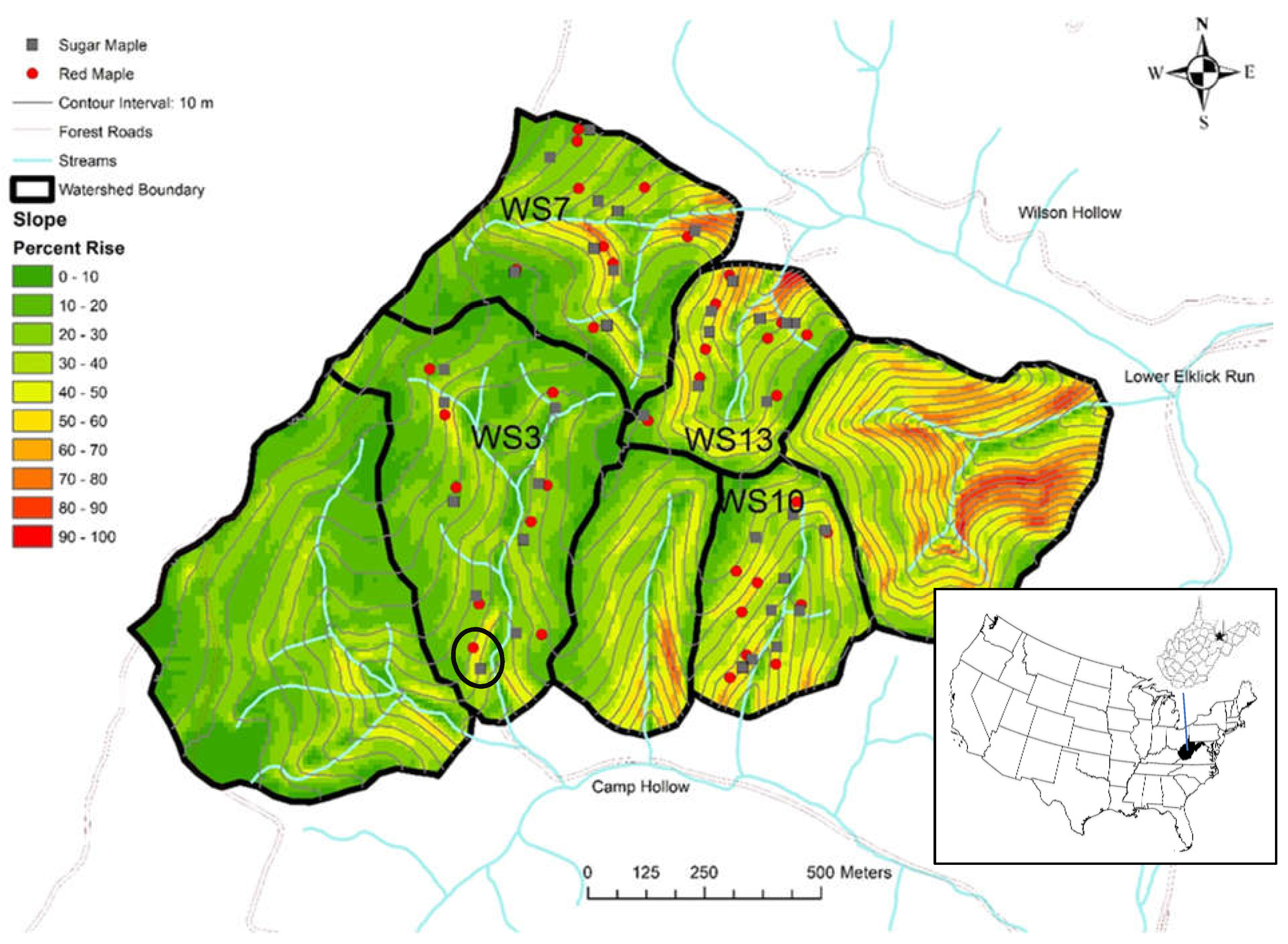
2.1. Study Site

This study was conducted at the Fernow Experimental Forest (FEF), located in Tucker County in north-central West Virginia (Figure 1), in 2018 and 2019. The FEF lies within an area classified as the Allegheny Mountain Section of the Central Appalachian Broadleaf Forest [40]. The growing season extends from May through October, with tree leaves emerging in late April and being fully developed by mid-June. Leaves begin to fall in late August to early September. The mean annual precipitation is approximately 1460 mm with most precipitation occurring during the growing season (March through August) [41,42]. During the sampling periods (Apri–August) of 2018 and 2019, total precipitation was 914 mm and 842 mm, respectively. These amounts are in the upper 20th percentile of amounts recorded since 1990, averaging 708 mm for this 30-year period. Mean monthly air temperatures range from −2.8 °C in January to 20.4 °C in July [43]. In 2018 and 2019, the mean July temperatures were 20 °C and 20.5 °C, respectively. The most common soil at FEF is Calvin channery silt loam (loamy-skeletal, mixed, active, mesic Typic Dystrudept) [43] derived from acidic sandstone parent material. In the top 10 cm of mineral soil, soils comprised about 67% sand, 22% silt, 11% sand, and 14% organic matter [33]. In the top 5 cm of the mineral soil, average pH (CaCl2) is 3.7 (range 3.0–4.4), % C is 5.5 (range 1.9–12.5), % N is 0.35 (range 0.15–1.0) [44]. Dominant overstory species at the FEF are sugar maple, sweet birch (Betula lenta L.), American beech, tulip-poplar, black cherry, and northern red oak (Quercus rubra L.) [45].
Four experimental watersheds (WS) in close proximity to each other (WS3, WS7, WS10, WS13) were included in this study (Figure 1). These watersheds support closed-canopy forest and are similar with respect to elevation, soil series, geology, climate, and most of their disturbance history. Watersheds were heavily logged around 1910 (along with most forests of West Virginia) [46] and then left to regenerate naturally [47]. American chestnut (Castanea dentata (Marshall) Borkh.), a dominant species at the time, was harvested from the watersheds in this study in the 1940’s, after the trees had died from the introduced chestnut blight [46]. Watersheds differed in their more recent anthropogenic disturbance history (detailed below) and watershed aspect (Table 1), providing the foundation for this study.
Watershed 3 (WS3) had received long-term fertilization/acidification treatments to study the effects of atmospheric N deposition. Since 1989, granular ammonium sulfate has been applied aerially three times a year at a rate of 7.1 kg N ha⁻1 in March and November, and 21.2 kg N ha⁻1 in July [40]. Partial cuts were made in 1958, 1963, and 1968, respectively removing 14%, 9%, and 6% of trees with a diameter at breast height (DBH) ≥ 12.7 cm. The watershed was subsequently clearcut in 1969–1970, removing all trees with a DBH ≥ 12.7 cm; all saplings with a DBH between 2.5 cm and 12.5 cm were sprayed with herbicide [46]. A 3-ha riparian/protection buffer strip (approximately 40 m wide and 730 m long) was initially left along the perennial stream to help protect water quality; it was cut in 1972 [41,48]. In 2003, the dominant tree species (as % basal area) in this watershed were black cherry (51), red maple (11.5), northern red oak (5.1), and sweet birch (5.1); sugar maple made up 1.3% of the total basal area in WS3 [49].
To assess fertilization/acidification effects in WS3, watershed 7 (WS7) was used as an unfertilized reference watershed due to similar disturbance history. The upper half of WS7 was clearcut from 1963–1964; the lower half was clearcut from 1966–1967. Following the clearcuts, the watershed was then treated annually with herbicide till 1969 [43]. In 2003, the dominant tree species (as % basal area) for this watershed were tulip-poplar (26.2), sweet birch (20.5), black cherry (20.5), red maple (8.2), and sugar maple (4.9) [45].
Watershed 10 (WS10) and Watershed 13 (WS13) served as “unmanaged” watersheds although a final, partial cut took place in WS13 in the early 1950s [47]. In 2000, the dominant tree species in WS10 (as % basal area) were chestnut oak (24), northern red oak (22) red maple (19), blackgum (Nyssa sylvatica Marshall, 8), and white oak (Quercus alba L., 6); sugar maple made up 2% of the total basal area in WS10. In WS13 dominant species were northern red oak (30), sugar maple (22), red maple (13), tulip-poplar (7), and American beech (7) [50]. WS10 and WS13 differ in watershed aspect (S vs. N, Table 1).

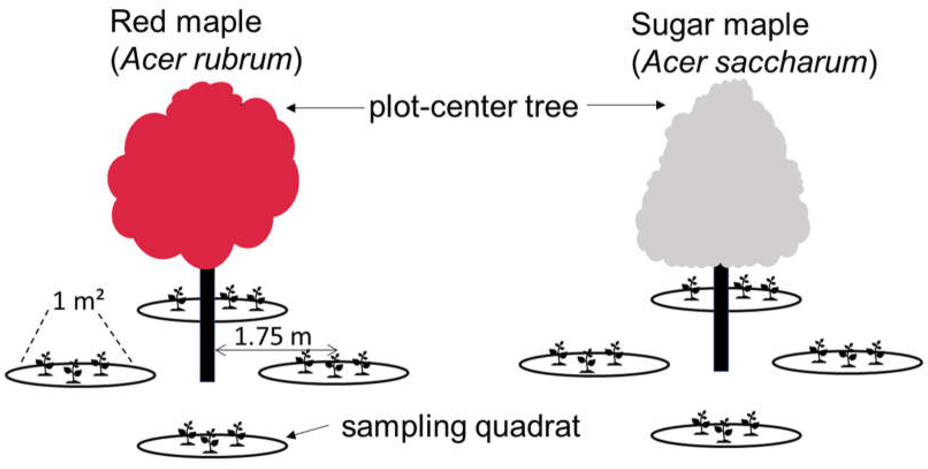
2.2. Experimental Design

To collect herb-layer data, a total of 18 plots were established in each of the four watersheds. Two adjacent plots, with one centering around a stem of sugar maple and the other around a stem of red maple, represent a site (Figure 1 and Figure 2). Prior to selecting maples for this study, a total of 151 maple trees had been located, if possible, upslope from the riparian area and downslope from the watershed boundary (to minimize variability due to a moisture gradient). In each watershed, at least twice as many trees per species were initially located than were used in this study. Tree locations were recorded with GPS and mapped. From this map, sites were identified if a red and sugar maple tree were reasonably close, and of those sites, four or five were randomly selected on either side of the main stream (totaling nine sites per watershed). The distance between plot centers of a red and sugar maple pair averaged 32.5 m (range: 6.2–83.1 m) while the average distance between neighboring plot pairs (closest plot centers) was 112.6 m (range: 16–257.9 m) (Figure 1). Selected plot-center trees were vigorous (i.e., without signs of disease or injury) and had a DBH ≥ 10 cm (average DBH 20 cm, range 10 cm–41 cm).

2.3. Data Collection and Analysis

Cover of herb-layer species (<1 m tall) were assessed in four circular 1-m2 sampling quadrats established at the four cardinal directions (N, S, E, W) from the plot-center tree (Figure 2). Sampling quadrats represented subsamples of the plot; therefore, cover was averaged across the four quadrats per plot prior to analysis. The center of the sampling quadrats was 1.75 m away from the base of the plot-center maple, roughly halfway between the stem and the edge of the crown to avoid stem flow and canopy drip. Each quadrat location was marked with three stake flags on the perimeter so that sampling quadrats could be placed in exactly the same spot during the different sampling campaigns. Herb-layer species composition and cover were collected in early summer 2018 (16 June–5 July), spring 2019 (3 May–6 May), and summer 2019 (29 June–29 July). Environmental variables that may influence the herb layer (slope angle, aspect, slope position, canopy cover, DBH of plot-center maple, DBH of neighbor trees) were collected from June through August 2018; as an exception, leaf area index (LAI) was collected on August 6 and September 5, 2019.
Within each sampling quadrat, herb-layer composition was determined by identifying plants to species level, with exceptions for grasses and sedges (identified as graminoids), and Rubus L., Viola L., and Anemone L. (identified to genus level). These taxonomically difficult groups were not identified to species level to limit misidentification. For example, at the FEF, the vast majority of Rubus individuals are R. allegheniensis (Allegheny blackberry), but R. idaeus L. (common red raspberry) also occurs at this location. Rubus species can hybridize and are difficult to identify without fruit or flowers [32]. These exceptions might have resulted in an underestimation of species richness but had little influence on the other diversity indices since graminoids and Anemone had very low abundances and Rubus likely was R. allegheniensis.
For each taxon, cover was measured as leaf area using the hand-area (HA) method [51]. In brief, the HA method compares the area of a hand with the area of the leaves of all plants of a given species. The observer places a hand (equivalent to 1% of 1 m2), palm down and fingers closed, directly above the leaves or leaflets of the species of interest and then determines the size of the leaf in relation to their hand, either as individual or group, until all leaf surfaces are observed within the quadrat. To improve the accuracy and precision, (a) observer hands were calibrated to 1 dm2 by folding under the thumb and or fingertips depending on the actual size of the observer’s hand and (b) two observers independently recorded cover, with the average of the two estimates being recorded [51]. Cover was estimated with a precision of 0.01% (i.e., 1 cm2 leaf area in the 1-m2 quadrat).
Species richness (S), Shannon–Wiener diversity index (or Shannon index, H), and Pielou’s evenness (J) were calculated at the plot level. Species richness is the number of species per unit of area, i.e., in this study, S is the total number of species found across the four sampling quadrats per plot. Shannon index is commonly used to characterize species diversity, which accounts for both abundance and evenness of species present [52]. H will increase with increasing species richness and with increasingly equitable contributions of the species to the community. Pielou’s evenness is another measure of diversity. Values for J are the ratio of actual H to maximally possible H (if all species were present in equal proportion) [52,53].
The Shannon index is calculated as
H = i = 1 s P i ln P i
where Pi is the relative abundance of each herbaceous species in the plot and where s is the number of species [54].
Pielou’s evenness is calculated as
J = H H m a x = H / ln S
where H is the Shannon index and S is the total number of species [53].
To characterize the abiotic environment of the herb layer, several variables relating to light availability, soil moisture, and temperature were measured in each plot. To quantify the light environment above the herb layer, percent canopy cover was measured with a densiometer over each sampling quadrat while facing the plot-center tree. LAI was measured in the same locations (albeit in 2019) using an Accupar LP-80 PAR/LAI ceptometer (Meter Group, Inc., Pullman, WA, USA) (details in [55]). The four respective densiometer and LAI measurements were then averaged for each plot. Slope (%) was measured using a clinometer and aspect (°) was determined with a compass; both measurements were taken at the plot center facing downhill. Slope position, assumed to correlate with soil moisture, was measured in ArcMap as the slope distance from the plot center to perennial stream. To align aspect with ecologically relevant effects of radiation (e.g., heat and moisture balance), and to be able to analyze it as a continuous variable, aspect was transformed into a linear scale that ranges from 0 to 2, with 0 being the relatively warmer and drier southwest and 2 being the relatively cooler and moister northeast, using the formula:
A = sin ( A + 45 ) + 1
where A′ is the transformed aspect code and A is the aspect defined as the direction of the prevailing slope [56].
To assess the potential influence of neighboring trees on herb-layer characteristics, DBH of the five closest neighboring trees (>2 m height) was measured. For each neighbor tree, ectomycorrhizal (ECM) or arbuscular mycorrhizal (AM) association was determined (based on [57,58]), and basal area (BA, cm2) was summed for each association. The average distance of the farthest tree from the plot center was 5.7 m (range 2.9–11.6 m).

2.4. Statistical Analysis

The relationships between herb-layer composition, watersheds, overstory maple, and environmental variables in summer 2018, were analyzed with a constrained ordination (i.e., direct gradient analysis including species and environmental data) in Canoco 5.1 [59]. In a constrained ordination, only the species composition variability is shown that can be explained by environmental variables. Specifically, canonical correspondence analysis (CCA) was performed with forward selection of significant predictor variables. Most of the environmental variables were not highly correlated with each other (VIF < 3.3). However, DBH of the largest neighbor tree and BA of ECM trees had a VIF of 11.3 and 7.9, respectively. These variables were highly correlated with each other (0.83) and moderately correlated with WS13 (0.61 for large neighbor DBH and 0.65 for BA of ECM trees).
In the analysis of community-level indices (cover, S, H, J), analysis of variance (ANOVA) was conducted separately for watershed pairs. Watershed pairs were WS3-WS7 (treatment: fertilization level; same, “younger” stand age); WS7-WS13 (treatment: stand age; similar aspect); and WS10-WS13 (treatment: watershed aspect; same, “older” stand age). The analysis of watershed pairs reduced the potential for confounding the intended watershed-level treatment (e.g., fertilization) with other differences between watersheds (e.g., stand age). Residuals of response variables were checked for normality; response variables did not require transformation. After detecting extreme observations in some predictor variables (distance-to-stream, BA of ECM trees, BA of AM trees) when conducting influence diagnostics in regression analyses, these variables were square-root-transformed to reduce the influence of high-leverage extreme observations in model predictions. No significant multicollinearity was detected between the continuous environmental variables (VIF < 10). Using JMP and SAS (JMP®, Version Pro 12.2, SAS Institute Inc., Cary, NC, USA, Copyright ©2015; SAS®, Version 9.3, SAS Institute Inc., Cary, NC, USA, Copyright ©2002–2010), analyses were conducted separately for the spring and summer datasets. For the spring dataset, repeated measures analyses of variance were undertaken to account for the spatial correlation between sugar maple/red maple plot pairs within a site (Figure 1) (SAS code: Repeated Tree/Subject = Site * WS). Datasets from summers 2018 and 2019 were jointly analyzed in a doubly repeated ANOVA accounting for the spatial relationships of plot pairs and the repeated measurement in time (SAS code: Random Tree/Subject = Site * WS; Repeated Year/Subject = Tree * Site * WS). Models evaluated the effects of watershed-level treatment (factor Watershed, WS), plot-center overstory maple species (factor Maple, M), their interaction (WS × M), and variables describing the physical and biotic environment on each herb-layer characteristic (cover, S, H, J) (Table 2). Thus, 12 models (three watershed pairs × four herb-layer indices) were run for the summer and spring data, respectively. A reduced model was created from the full model by removing predictor variables (other than WS, M, WS × M) with high p-values (i.e., p > 0.4); applying a backward elimination regression was not possible due to not all predictor variables being continuous variables. Final model selection (i.e., choosing between the full versus reduced model) was determined by the lowest AIC value. Graphs and tables show untransformed raw data.
Within each watershed pair, pairwise comparisons of herb-layer indices were conducted (a) between the two overstory maple species per watershed and (b) between the two watersheds under a given overstory tree species. There was no adjustment made for multiple comparisons, but the number of comparisons were minimized (to four, using the Slice function in SAS) to reduce false positives (Type I error). In all statistical analyses, significance criterion alpha was 0.05 and a statistical trend was declared when p ≤ 0.1.
To determine associations between individual herb-layer plant species with watershed and overstory maple species, ANOVA was conducted separately for 22 frequent herb-layer species in each of the three watershed pairs. Since the probability of a Type I error increases with the number of tests conducted (familywise error rate), the Benjamini–Hochberg method was applied to control the false discover rate (i.e., a false positive or a Type I error). The concept is similar to the Bonferroni adjustment for multiple comparisons, yet less conservative [60]. To perform the Benjamini–Hochberg method, individual p-values from ANOVAs are ranked from smallest to largest. The smallest p-value receives a rank (i) of 1, the next larger p-value receives the rank of 2, etc. Next, each p-value is compared to the Benjamini–Hochberg critical value (i/m)Q, where i is the rank, m is the total number of tests (total number of individual p-values ranked), and Q is the false discovery rate selected by the researcher [60]. In this study, the false discovery rate was set at 0.10. For the cover of a plant species to vary significantly by WS, M, or WS × M, the p-value must be smaller than the Benjamini–Hochberg critical value. For example, with 22 species and two main effects (WS, M) and an interaction effect, there is a family of 66 analyses (i.e., m = 66). For the smallest p-value obtained by ANOVA to be considered significant, it would have to be smaller than 1/66 × 0.1 = 0.0015; the p-value at rank two would have to be smaller than 2/66 × 0.1 = 0.003, etc. The largest p-values that is smaller than the Benjamini–Hochberg critical value, and all of the p-values smaller than it, are considered significant [60].
While the analyses of the overstory maple species effect on herb-layer indices and the cover of individual species are truly replicated, the analyses of differences between watersheds are pseudo-replicated, i.e., no inference can be made beyond the watershed pairs used in this case study.

3. Results

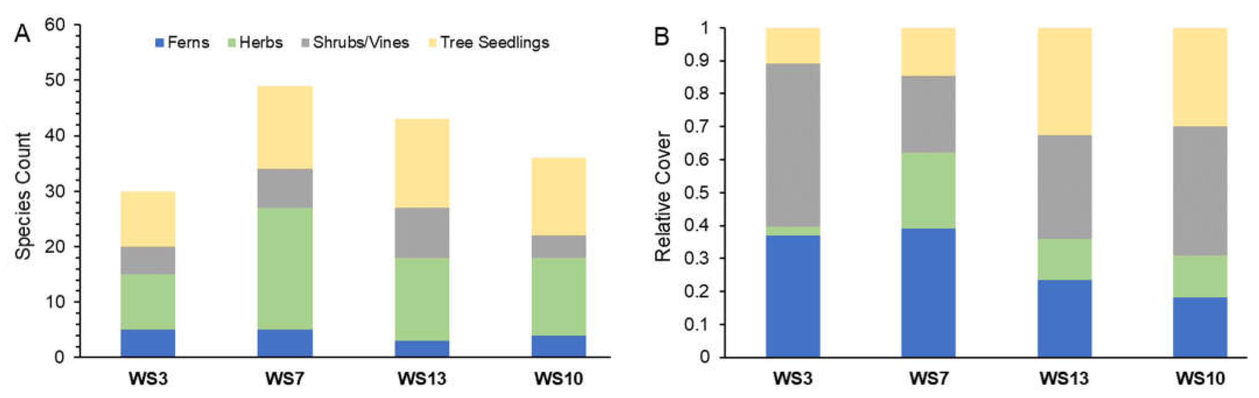
3.1. Community Composition

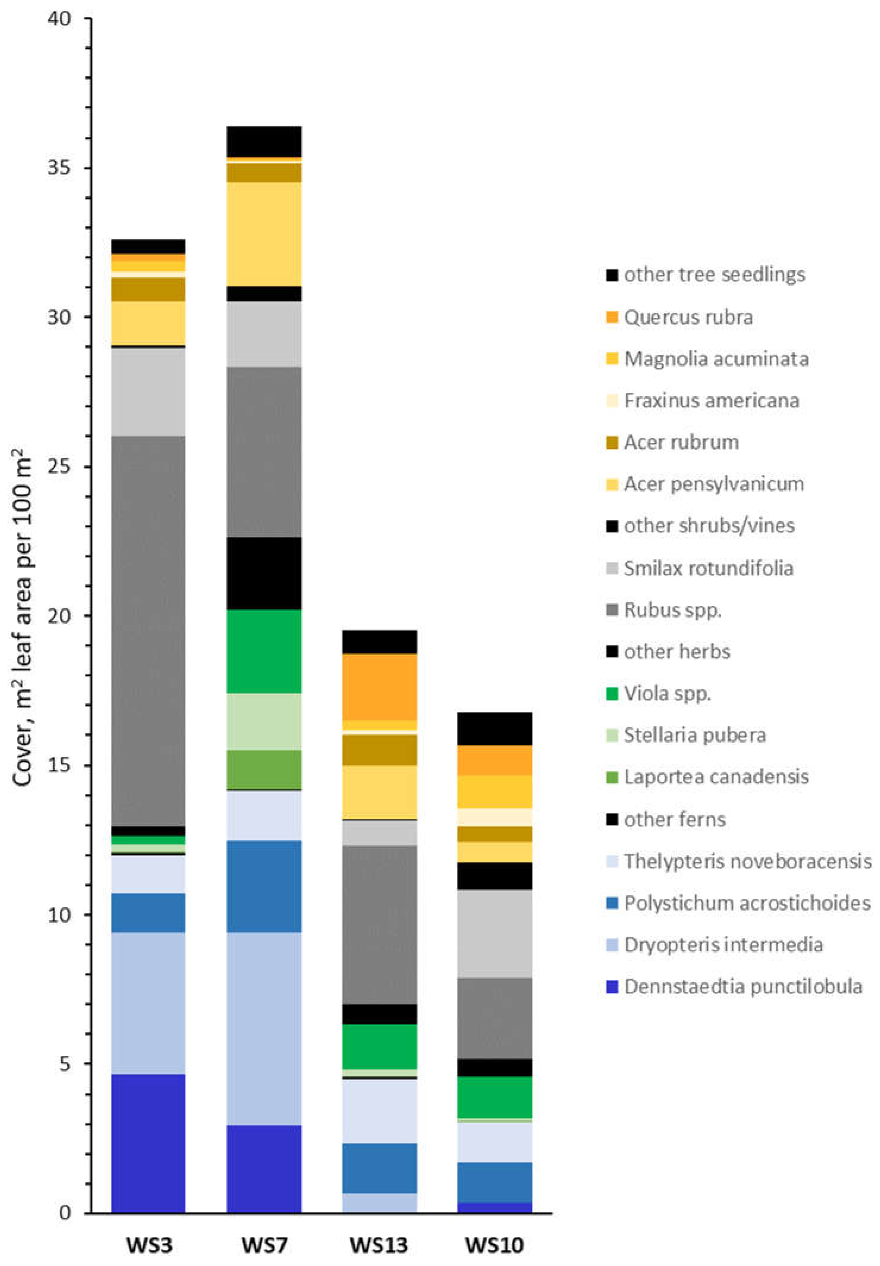
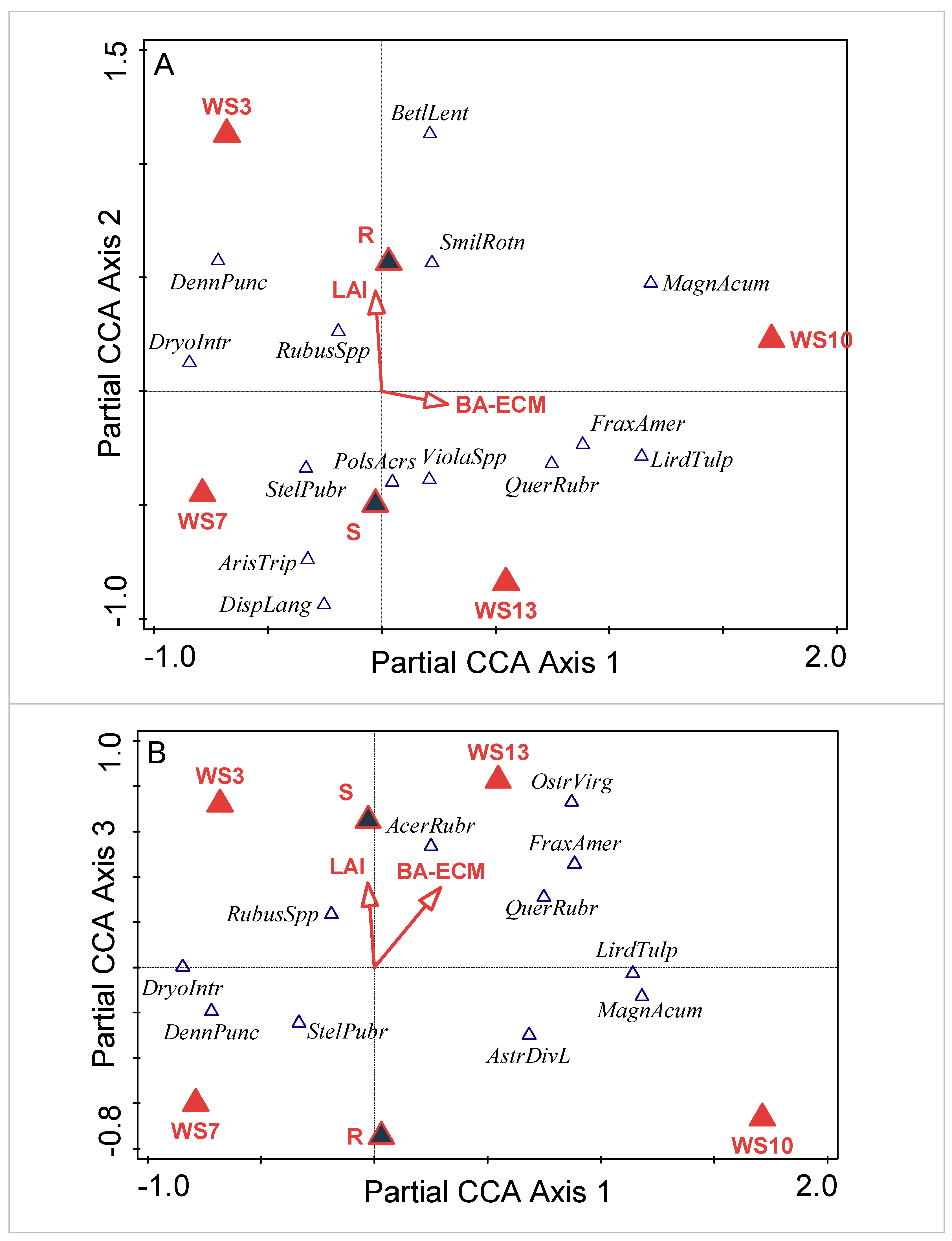
3.1.1. Watershed-Level Herb-Layer Community Composition

Among all four watersheds, a total of 63, 57, and 64 taxa (including three genera and not counting graminoids) were recorded during the summer 2018, spring 2019, and summer 2019 sampling periods (Table 3, Table S1), respectively. Except for multiflora rose (Rosa multiflora Thunb. ex Murr.) and Japanese barberry (Berberis thunbergii DC.), all herb-layer species were native species. Species numbers were consistently highest in WS7 (younger stand, unfertilized), lowest in WS3 (younger stand, fertilized), and intermediate in WS10 and WS13 (older stands) (Table 3, Figure 3A). Herb-layer indices were similar between sampling periods, likely due to most species being perennials and resampling the same quadrats. Cover was expectedly lower in spring than in summer (Table 3). In all watersheds, most herb-layer species were tree seedlings or herbs (Figure 3A) with similar proportions of species in each plant type (fern, herb shrub/vine, tree seedling) between the watersheds (Table S2). However, the absolute number of herb and tree species (as seedlings) was lower in WS3 (younger stand, fertilized) than in the other watersheds (Figure 3A). Watersheds also differed in the proportion of total cover in different plant types. The younger stands (WS3, WS7) had a higher proportion of cover in ferns than the older stands (WS10, WS13). Comparing the two younger stands, half of the cover in fertilized WS3 was due to shrubs/vines and less than 3% of all cover was due to herbs, whereas the contribution to cover from these two plant types in WS7 was about equal (Figure 3B). Blackberry, intermediate shield fern (Dryopteris intermedia (Muhl. ex. Willd.) Grey), and hay-scented fern (Dennstaedtia puntilobula (Michx.) Moore) made up two thirds of all cover in WS3 (Figure 4), which is reflected in a lower Shannon index and evenness than in the other watersheds (Table 3). The 14 species with the highest relative cover in the study area contributed 97%, 89% 85%, and 93% to the total cover in WS3, WS7, WS10, and WS13, respectively (Figure 4).

3.1.2. Plot-Level Herb-Layer Community Composition

At the plot level, multivariate analysis (CCA) with forward selection of significant predictor variables and factors levels revealed that factor Watershed, factor Maple (red vs. sugar maple), and four environmental variables (LAI, basal area of ectomycorrhizal neighbor trees—BA-ECM, aspect code, distance to stream) were significant (p ≤ 0.1) in explaining variability in herb-layer species composition. Of the total variability in species composition, the selected predictor variables together could explain 19.5%. While this number is low, it is not unusual because species data are inherently noisy [61]. Individually, factor Watershed explained 10.3%, the group of four environmental variables explained 8.5%, and factor Maple explained 2.2% of the total variability in the species data.
While influencing species composition, the physical attributes of the plots (e.g., slope angle, plot-level aspect, and slope position [i.e., distance to stream]) were not of primary interest and were subsequently analyzed as covariates in a partial CCA. After removing the compositional variability explained by physical plot attributes, the remaining explanatory factors/variables (Watershed, Maple, LAI, BA-ECM) together accounted for 16% of the total variation in the species data. Conversely, the group of physical plot attributes explained 6.8% of variation in herb-layer species data when Watershed, Maple, LAI, and BA-ECM were used as covariates.
Most (76%) of the variation in species composition (explained by Watershed, Maple, LAI, and BA-ECM) was represented by the first three canonical axis (Figure 5A,B). Species composition in WS3 (fertilized, younger stand) was most dissimilar from WS10 and WS13 (unfertilized older stands); unfertilized WS7 had a species composition similar to fertilized WS3 of the same stand age and WS13 of older stand age but same fertilization status (Figure 5A). The proximity of species symbols for blackberry, intermediate shield fern, and hay-scented fern to the symbols for WS3 and WS7 indicated the species’ higher relative abundance in these watersheds (with younger stand age). Star chickweed (Stellaria pubera Michx.), violets, yellow fairybells (Prosartes lanuginosa (Michx.) D.Don) and jack-in-the-pulpit (Arisaema triphyllum (L.) Schott) had higher relative abundances in unfertilized WS7 than fertilized WS3. Tree seedlings had a higher relative abundance in plots of WS10 and WS13 (older stand age) than in WS3 and WS7 (younger stand age). The somewhat different species compositions under red maple compared to sugar maple is shown by the separation of these factor levels along Axes 2 and 3 (Figure 5A,B). Plots of WS10 and WS13 (older stands) were separated from the plots of WS3 and WS7 (younger stands) along Axis 1 that correlated with the basal area of EM-associated trees among the five nearest neighbors of the plot-center maple (Figure 5A). Among the younger stands, plots of fertilized WS3 were separated from plots of unfertilized WS7 along Axis 2 that mainly correlated with LAI (Figure 5A). BA of ECM trees was highly (0.83) correlated with the DBH of the largest neighboring trees, a variable that therefore likely did not come up as significant in the forward selection. Factor level WS13 was moderately positively correlated with BA-ECM (0.56) and DBH of the largest tree neighbor (0.6), and factor level WS3 was moderately positively correlated with LAI (0.45). This suggests partial mechanisms for watershed-level differences. Interestingly, red maple seedlings (found in nearly all plots, Table S1) had higher cover under sugar maple than under red maple (Figure 5B) and no seedlings of sugar maple were found in plots in the fertilized watershed.

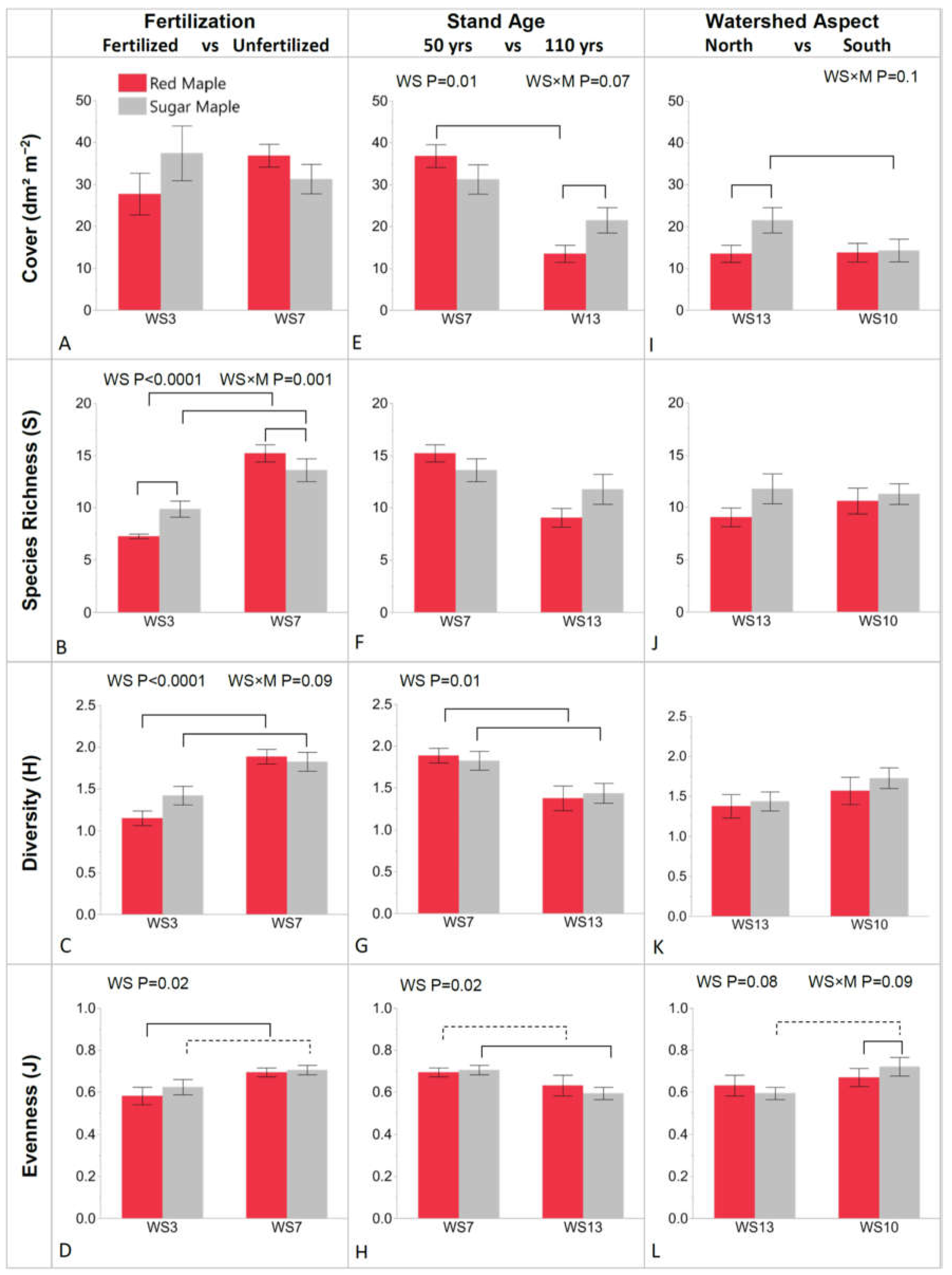
3.2. Herb-Layer Indices: Cover, S, H, and J

The importance of factors watershed, maple, and environmental variables was also reflected in herb-layer community-level indices (cover, S, H, J). In the ANOVAs of summer herb-layer cover, S, H, and J in watershed pairs, factor Watershed (WS), in the sense of “treatment”, affected the herb layer in watershed pairs WS3 vs. WS7 (fertilized vs. unfertilized) and WS7 vs. WS13 (younger vs. older stand age), but not in watershed pair WS10 vs. WS13 (south-facing vs. north-facing watershed aspect). Factor maple (M) was not statistically significant as a main effect in any of the models, but there was a statistically significant effect or a trend of the WS × M interaction in five of the 12 models (Table S3a). In these models, herb-layer cover, species richness, and/or Shannon–Wiener diversity were lower under red than sugar maples in one of the watersheds in the pair (WS3, WS13) but not the other (WS7, WS10).

3.2.1. WS3 vs. WS7: Fertilized vs. Unfertilized 50-Year-Old Stands

In the comparison of the fertilized and unfertilized watersheds (both with 50-year-old stands), factor Watershed and/or WS × M interactions were statistically significant predictors for all herb-layer indices except cover. Species richness, diversity, and evenness overall were lower in fertilized WS3 than unfertilized WS7 (WS: p < 0.001, p < 0.001, p = 0.02, respectively) (Figure 6B–D, Table S3a). Species richness and diversity tended to be greater under sugar maples than red maples in fertilized WS3 with an opposite pattern or no difference between maples in the unfertilized WS7 (WS × M: p = 0.001, p = 0.09, respectively) (Figure 6B,C).
Analyses of individual herb-layer species showed that cover of three species varied with watershed or overstory maple species. Violets (Viola spp.) and jack-in-the-pulpit (Arisaema triphyllum L.) cover was significantly lower in fertilized WS3 than in unfertilized WS7 (WS: p = 0.001 and p = 0.003, respectively; Table S3). The cover of New York fern (Thelypteris noveboracensis L.) was greater beneath sugar maples than red maples in fertilized WS3 with an opposite pattern in WS7 (WS × M p = 0.002; Table S4).
Various environmental factors explained significant variation in herb-layer indices (Table S3a). S, H, and J decreased with increasing slope (p = 0.01, p = 0.004, p = 0.03, respectively), increased with increasing aspect code (i.e., aspect changing from southwest toward northeast) (p = 0.04, p = 0.02, p = 0.02, respectively), and decreased with increasing distance from the stream (p = 0.01, p = 0.01, p = 0.05, respectively) (Table S3a).

3.2.2. WS7 vs. WS13: Stand Age of 50 Years vs. 110 Years

In comparison of the two watersheds with different stand ages, factor Watershed was a statistically significant predictor for all community indices but species richness. Herb-layer cover was greater in WS7 (younger stand) than in WS13 (older stand) (WS p = 0.01). Cover tended to be higher under sugar maple than under red maple in the older stand, with an opposite pattern in the younger stand (WS × M p = 0.07) (Figure 6E, Table S3a). Diversity and evenness were higher in the younger stand (WS p = 0.01 and p = 0.02, respectively) than the older stand and did not vary by overstory maple species (WS × M p > 0.05) (Figure 6G,H; Table S3a).
Considering individual understory species, the cover of red maple seedlings was greater beneath sugar maples than red maples in both watersheds (M p = 0.0003; Table S4).
Four environmental variables showed a trend (i.e., p < 0.1) in explaining herb-layer indices, but none of the variables was consistently significant across multiple indices (Table S3a).

3.2.3. WS13 vs. WS10: Northerly vs. Southerly Watershed Aspect in 110-Year-Old Stands

In comparison of the two watersheds with the same older stand age but varying watershed aspect, factor Watershed, factor Maple, or their interaction (WS × M) were not statistically significant predictors for any of the herb-layer characteristics. There was a statistical trend of herb-layer cover under sugar maples being greater than under red maples in the north-facing watershed (WS13), while there was no difference in cover under the different maple species in the south-facing watershed (WS10) (WS × M p = 0.1) (Table S3a, Figure 6I). Evenness tended to be greater under sugar than red maples in WS10, with an opposite pattern in WS13 (p = 0.09) (Figure 6L). Species richness and diversity did not differ between watersheds (Figure 6J,K) (Table S3a).
Considering individual understory species, the cover of red maple seedlings was greater beneath sugar maples than red maples (M p = 0.0003) (Table S4). Environmental factors explaining significant variation (or a trend) in more than one herb-layer characteristic were plot-level aspect code and DBH of the plot-center maple. Herb cover increased and evenness decreased with increasing aspect code (p = 0.09 and p = 0.01). Diversity and evenness decreased with increasing DBH of the plot-center maple (p = 0.09 and p = 0.03) (Table S3a).
For all watershed pairs, spring herb-layer indices (Table S3b, Figure S1) were generally similar to summer herb-layer indices with the exception of expectedly lower cover.

4. Discussion

Plant communities are complex, which often results in noisy data sets. Nevertheless, this study showed that herb-layer composition and community indices can be affected by numerous factors, including abiotic environmental factors such as plot-level aspect and slope (expected results), overstory tree species (a novel finding), and anthropogenic activities, such as fertilization and land use history (i.e., stand age).

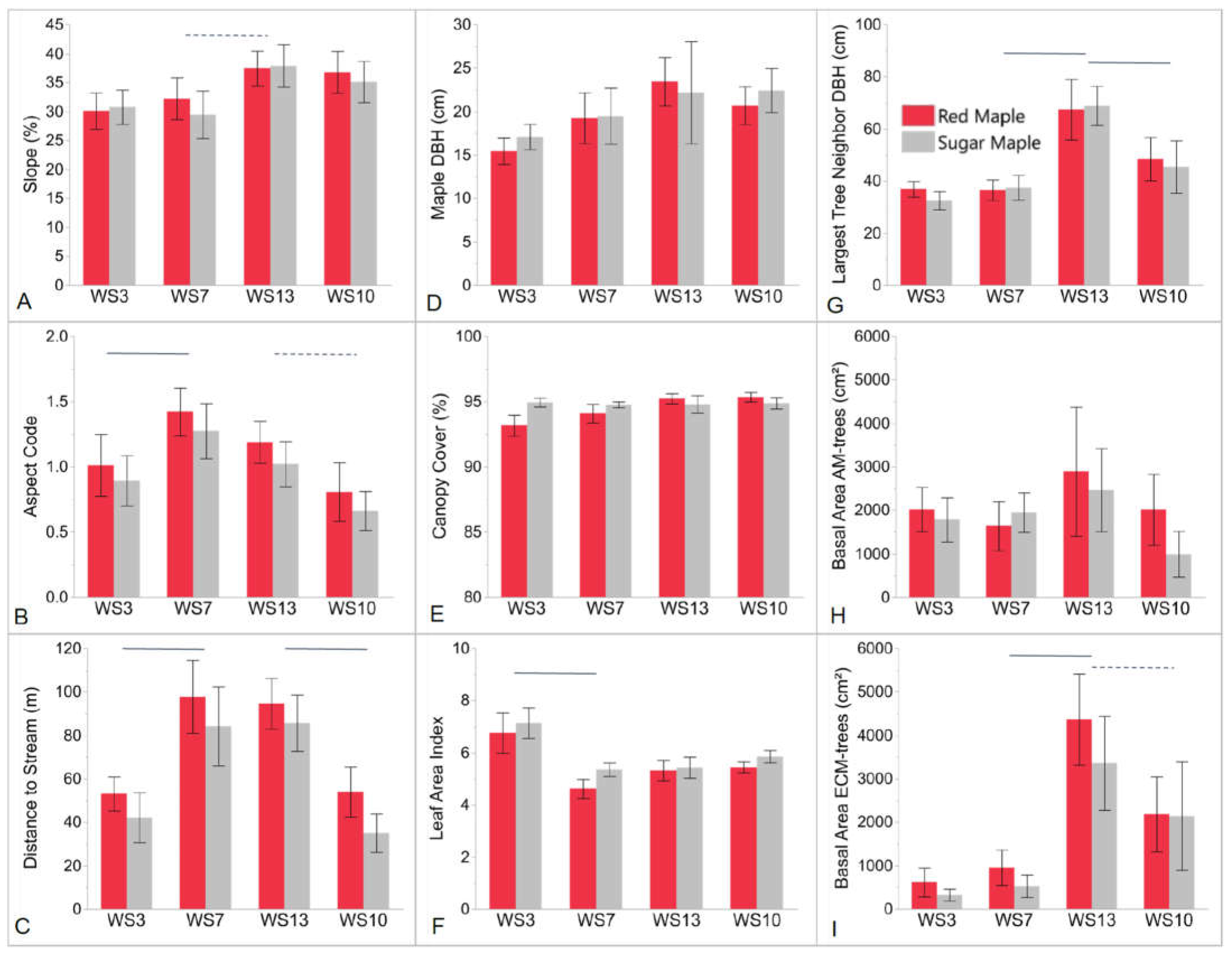
4.1. Influence of Abiotic Environmental Factors

The influence of abiotic factors that affect plant resources (e.g., soil moisture) has long been established in shaping plant communities. Therefore, it was not surprising to most frequently find a positive relationship of aspect code (i.e., increasing moisture availability) and negative relationships between slope steepness or plot distance to stream and the herb-layer indices (cover, S, H, or J) in the mountainous terrain of the FEF (Table S3a,b). A partial CCA indicated a relatively smaller importance of these abiotic variables compared to the group of predictor variables containing watershed-level treatment (fertilization, stand age, watershed aspect) and biotic variables (plot-center maple species, LAI, and basal area of ECM trees) in this study.

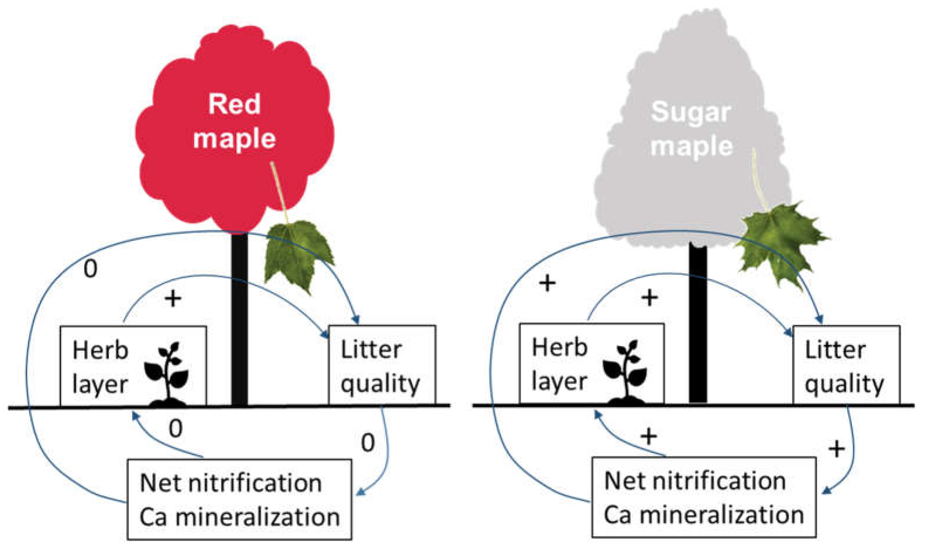
4.2. Herb-Layer Responses to Overstory Red Maple vs. Sugar Maple

Linkages between the overstory and the herb layer have been suggested to exist at spatial scales smaller than the landscape scale and may arise from parallel responses of strata to similar environmental gradients (e.g., soil pH, soil fertility, light) [19]. At the tree scale, this study revealed that the identity of the overstory tree species has a small but significant influence on the composition of the herb layer growing underneath (Figure 5). This response was more difficult to detect when the herb-layer composition was summarized into indices. There was no consistent response of the herb layer to the plot-center maple species across all watersheds; however, in summer (but not spring) the herb-layer response differed by maple species depending on the watershed. In five of the 12 models (four indices and three watershed pairs) there was a significant effect or trend of the WS × M interaction, indicating that the herb layer in summer benefitted from being under sugar maple relative to red maple in fertilized WS3 (50-year-old stand) and unfertilized WS13 (110-year-old north-facing stand), but not in unfertilized WS7 (50-year-old stand) and unfertilized WS10 (110-year-old south-facing stand) (Figure 6).
With none of the abiotic or biotic environmental variables measured in this study differing between red and sugar maple plots (Figure 7), mechanisms of a sugar maple effect on the herb layer may be located belowground. Since this study was not designed to establish causation of how individual tree species influence the herb layer (a heretofore unknown linkage), we can only speculate that differences in nutrient cycling below red and sugar maple may be a contributing factor (Figure 8). A positive feedback between litter quality and soil nutrient concentrations has been widely described (e.g., [63]). Soils beneath sugar maple have significantly less forest floor biomass (due to more rapid decomposition), a lower C:N ratio in the mineral soil layer [22,64], and significantly more calcium than soils under red maple [64,65]. At the FEF, sugar maple is associated with soils that have higher rates of nitrification and nitrate production than red maple [18]. With high mobility, nitrate may be more easily accessible to understory plants, but it is also susceptible to leaching [66]. Nitrification slightly decreases the pH of the soil, resulting in increased concentrations in soil solution and, thus, mobility of cations, such as calcium [67], which may benefit the herb layer under sugar maple (Figure 8).
Mycorrhizal fungi play an important role in the nutrition of forest trees and many herb layer species [68]. Mycorrhizae may, in fact, tighten the plant litter-soil feedback loop by facilitating more direct plant access to litter nutrients that otherwise would cycle first through the soil organic matter pool [69]. Since maples and most forest herbs are both associated with AM fungi [57,70], the linkage between these trees and their surrounding herb layer maybe a direct one via hyphal connections. While the fungal benefit from connections to multiple plant species lies in increased access to carbon, the benefits to the connected plants are not yet clear. It may be possible that “cheater” plants obtain their mineral nutrients from fungi at a lower carbon expense than other plants that provide relatively more carbon to the shared mycelium [71]. On native soil, red maple compared to sugar maple has been shown to have higher levels of mycorrhizal colonization [72]; whether this has any relevance to the herb layer is an avenue for exploration.
This study indicates that a sugar maple effect on the herb layer may not manifest under some conditions such as those in the younger unfertilized stand (WS7) and the older unfertilized stand with a southerly watershed aspect (WS10). It is possible, that in these watersheds a sugar maple effect is masked by other factors (e.g., stand age, watershed aspect). These factors may influence the herb layer via soil nutrient cycling (as reflected in differing stream water nitrate concentrations, Table 4). Under conditions of high external N inputs in WS3, sugar maple may be able to buffer—at the tree scale via litter-soil feedback—against potential nutrient imbalances at the watershed scale following excessive nitrate and calcium leaching (Table 4, [73]).

4.3. Herb-Layer Responses to Fertilization: WS3 vs. WS7

In this study, the herb-layer diversity indices (S, H, J) were consistently negatively affected by long-term N amendments to WS3 compared to unfertilized WS7. As the applied fertilizer was ammonium sulfate, changes in the understory may reflect direct responses to NH₄+ or concomitant changes in soil properties (i.e., soil acidification, calcium loss; [73]), and indirect responses via competitive exclusion from nitrophilic species [33] or high LAI (Figure 7F). Interestingly, the tree canopy in fertilized WS3 was taller and more open than in unfertilized WS7 [75], which may have ameliorated potential LAI effects on the herb layer in fertilized WS3. Additionally, the average aspect code indicated a somewhat moister microclimate in unfertilized WS7 than fertilized WS3, and plot-center maples were located closer to the stream in fertilized WS3 than unfertilized WS7 (Figure 7B,C). These differences could, in part, be confounded with a fertilization effect. Alternatively, in WS3, the lower slope positions, where maples were found, may have been in compensation for the overall southerly watershed aspect (relative to WS7) without affecting the herb-layer indices measured in this study.
The lower values for S, H, and J in the fertilized than unfertilized watershed are predicted by the N homogenization hypothesis [29], stating that, as an ecosystem shifts from N limitation to N saturation, species richness decreases due to the displacement of N-efficient species by nitrophilic species. In this study, as in the study of Gilliam et al. [33], N-efficient species were displaced by species such as Rubus spp., altering community composition and decreasing biodiversity. The N homogenization hypothesis also states that the response time of the herbaceous layer to fertilization will depend on ambient N. For example, an environment with low N would react more quickly to additional N than an environment with high N. As sugar maple is known to be associated with higher soil N availability than red maple at the FEF [18], the vicinity of sugar maple could potentially delay the negative effects of fertilization on understory richness, diversity, and evenness. However, since fertilization began almost 30 years prior to this study, the sugar maple effect observed in this study is more likely due contemporaneous effects, e.g., sugar maple locally buffering against nutrient imbalances (Figure 8).
This study provided additional data to the research by Gilliam et al. [33] at the FEF comparing herb-layer characteristics during the first 25 years of N fertilization in WS3 to a different unfertilized watershed (WS4) with similar land use history as WS10/WS13. In their study, there was an increase in herb-layer cover in the fertilized watershed with a younger stand (WS3) in comparison to the unfertilized watershed with an older stand (WS4). In our study, the unfertilized watershed with a younger stand (WS7) also had a higher cover than the unfertilized watershed with the older stand (WS13) (Figure 6E). This indicates that the findings of Gilliam et al. [33] may also, at least in part, represent a stand age effect rather than solely a fertilization effect and, thus, highlights the need for careful selection of reference watersheds in case studies.

4.4. Herb-Layer Responses to Land Use History (Stand Age): WS7 vs. WS13

Herb cover and diversity indices (S, H, J) were consistently greater in the younger watershed (WS7) compared to the older watershed (WS13). The results of this study are in agreement with Bormann and Likens [76], who noted greater diversity in recently disturbed stands (25–75 years since disturbance) relative to mature stands at the Hubbard Brook Experimental Forest in New Hampshire. In a compilation of several studies on the effects of clearcutting on herb-layer richness and diversity (S, H) in northeastern US forests, effects varied between studies [77]. In 2-year to 26-year-old clearcuts, in comparison to mature second growth forest (55 to >150 years old), S and H were either higher than, or the same as, in clearcut sites than their reference sites. In contrast, S and cover of spring flora in secondary forests (stand age 45–87 years) of the southern Appalachian Mountains were lower than in old-growth reference stand [39].
Changes in species richness are influenced by stand development during succession after harvest, where initial high species richness is due to colonization of remnant shade-tolerant communities by shade intolerant herbs, followed by a decrease during the stem exclusions stage of stand development due to low light levels below the canopy, followed by an increase in the old-growth stage due to increases in canopy horizontal and vertical heterogeneity [77]. However, site conditions, such as soil fertility, may exert an overriding control on successional patterns of species diversity [77,78].
In this study, the two watersheds with different stand ages appeared to vary in soil nutrient resources. Stream water nitrate and calcium concentrations were higher in the younger stand (WS7) than in the older stand (WS13) (Table 4), which may reflect the high availability of these ions in soil solution prior to leaching. Higher nitrate concentrations in soil water 45 cm below the soil surface were found in the study plots of younger WS7 than older WS13 [55]. Since both watersheds are similar in their physical characteristics (Figure 7A–C), higher soil nutrient levels in WS7 than WS13 may be the result of the more recent disturbance. Mechanistically, this may be due to early successional tree species (black cherry, tulip-poplar) still dominating in WS7 50 years after harvest, whereas WS13 is dominated by oak (Table 1). In this study, neighboring trees, growing on average 4 m away from the plot-center maple (range 0.5–11.6 m), could influence the litter quality in the study plots. Surrounding the plot-center maples in WS13 were ECM trees (mostly northern red oak, Table 1) with a basal area about four times higher than ECM trees surrounding plots in WS3 (Figure 7I). Trees associated with ectomycorrhizal fungi produce litter that breaks down more slowly due to low N and P and high lignin content compared to arbuscular mycorrhizal trees [17,24,79]. The resulting feedback between low-quality litter and soil may affect the herbaceous layer by impacting nutrient access [69]. Further, while canopy cover and light levels above the herb layer (Figure 7E,F) were similar between the younger and the older stand, canopy structure might differ and might exert influence over the herb layer [80].

4.5. Herb-Layer Responses to Watershed Aspect: WS13 vs. WS10

For the two unfertilized watersheds with 110-year-old stands, there was no main effect (p ≤ 0.5) of WS, i.e., watershed aspect did not predict herb-layer indices. While the average aspect code and distance to stream differed between these two watersheds, they were only significant predictors for evenness, but not richness or Shannon–Wiener diversity index. This supports the interpretation of differences in richness and diversity between fertilized WS3 and unfertilized WS7 as fertilization effect rather than these watersheds’ differences in aspect code and plot distance to stream. Thus, while pseudo-replicated, the watershed-level differences of interest (i.e., fertilization and stand age) likely cause the differences in herb-layer indices in the comparisons of WS3 vs. WS7 and WS7 vs. WS13, respectively.

5. Conclusions

This study demonstrated (1) the possible existence of a sugar maple effect, i.e., sugar maple having a positive effect on herb-layer cover, (2) that long-term N enrichment can reduce ecosystem biodiversity by favoring nitrophilic plant species, (3) that herb-layer characteristics can be influenced by stand age, in that lower litter quality in later-successional stands (dominated by ECM trees, i.e., oaks) may lead to lower herb-layer abundance and diversity than in earlier successional stands dominated by AM trees, and (4) that watershed aspect did not influence herb-layer indices. While lower herb-layer cover and diversity indices in older relative to younger stands may be part of the natural successional trajectory in forests recovering from disturbance, lower herb-layer cover and diversity in the N-fertilized watershed indicates that anthropogenic activity may have fundamentally altered the overall structure and function of the eastern deciduous forest over the past decades of high atmospheric N deposition. Looking into the future, as maple species are shifting in abundance in the eastern United States [81] and atmospheric N deposition is decreasing in the eastern United States [82], concomitant change in the understory can be expected along with changes in ecosystem function due to feedback between diversity and productivity. Given the urgent need to adapt forest management to meet the challenges of climate change and other anthropogenic influences, this study justifies further examination of tree-herb layer interactions for a wider range of tree species, N-deposition levels, and stand ages in future studies.

Supplementary Materials

The following are available online at https://www.mdpi.com/article/10.3390/f12070829/s1; Table S1. Species found in each sampling campaign (Su—summer, Sp—spring) in studied watersheds (WS3, WS7, WS10, WS13) at the Fernow Experimental Forest, West Virginia, USA; Table S2. Proportion of the total number of species in different plant types at the watershed (WS) level at the Fernow Experimental Forest, West Virginia, USA; Table S3. Results of the statistical analyses (repeated measures ANOVA) of differences in herb-layer indices between watersheds (WS) at the Fernow Experimental Forest, West Virginia, USA, in (a) the summers of 2018 and 2019 and (b) the spring of 2019.; Table S4. ANOVA results testing the effect of watershed (WS), plot-center maple species (M) and their interaction (WS × M) for 22 individual herb-layer species found at the Fernow Experimental Forest, West Virginia, USA. The Benjamini-Hochberg method was applied to account for the familywise error rate; Figure S1. Spring 2019 plot-level herb-layer indices in red maple and sugar maple (M) plots in each of the studied watersheds (WS) at the Fernow Experimental Forest, West Virginia, USA.

Author Contributions

Conceptualization, K.S.; methodology, K.S.; formal analysis, L.J.S. and K.S.; investigation, L.J.S.; writing—original draft preparation, L.J.S. and K.S.; writing—review and editing, K.S.; visualization, L.J.S. and K.S.; supervision, K.S.; project administration, K.S.; funding acquisition, K.S. All authors have read and agreed to the published version of the manuscript.

Funding

This work was supported by the USDA National Institute of Food and Agriculture, McIntire Stennis Cooperative Research Program, project # WVA00129, the West Virginia Agricultural and Forestry Experiment Station, and a joint venture agreement (# 17-JV-11242303-065) with the USDA Forest Service, Northern Research Station.

Data Availability Statement

The data presented in this study are available on request from the corresponding author and at http://www.as.wvu.edu/fernow/data.html, accessed on 1 May 2021, Supplementary Material.

Acknowledgments

We thank Sian Eisenhut for field assistance, Ida Holaskova for supporting the statistical analyses, and the anonymous reviewers for improving the manuscript. We also thank the personnel at the Fernow Experimental Forest for maintaining and making available this outstanding research site and Mary Beth Adams and William Peterjohn for sharing their vast knowledge about the Fernow and the subject matter. Data on study site soil characteristics and basal area information of watersheds 10 and 13 were provided by William T. Peterjohn; these data were gathered as part of the Fernow Experimental Forest NSF LTRB awards DEB-0417678 and DEB-1019522.

Conflicts of Interest

The authors do not have any conflict of interest pertaining to this study.

References

  1. Gilliam, F. The ecological significance of the herbaceous layer in temperate forest ecosystems. Bioscience 2007, 57. [Google Scholar] [CrossRef]
  2. Muller, R.N. Nutrient relations of the herbaceous layer in deciduous forest ecosystems. In The Herbaceous Layer in Forests of Eastern North America; Gilliam, F.S., Roberts, M.R., Eds.; Oxford University Press: Oxford, UK, 2014; pp. 13–34. [Google Scholar]
  3. Hooper, D.; Chapin, F.S., III; Ewel, J.J.; Hector, A.; Inchausti, P.; Lavorel, S.; Lawton, J.H.; Lodge, D.; Loreau, M.; Naeem, S.; et al. Effects of biodiversity on ecosystem functioning: A consensus of current knowledge. Ecol. Monogr. 2005, 75, 3–35. [Google Scholar] [CrossRef]
  4. Allan, E.; Weisser, W.W.; Fischer, M.; Schulze, E.-D.; Weigelt, A.; Roscher, C.; Baade, J.; Barnard, R.L.; Beßler, H.; Buchmann, N.; et al. A comparison of the strength of biodiversity effects across multiple functions. Oecologia 2013, 173, 223–237. [Google Scholar] [CrossRef] [PubMed]
  5. Tilman, D.; Knops, J.; Wedin, D.; Reich, P.; Ritchie, M.; Siemann, E. The influence of functional diversity and composition on ecosystem processes. Science 1997, 277, 1300–1302. [Google Scholar] [CrossRef] [Green Version]
  6. Muller, R.N.; Bormann, F.H. Role of Erythronium americanum Ker. in energy flow and nutrient dynamics of a northern hardwood forest ecosystem. Science 1976, 193, 1126–1128. [Google Scholar] [CrossRef] [PubMed]
  7. Melillo, J.M.; Aber, J.D.; Linkins, A.E.; Ricca, A.; Fry, B.; Nadelhoffer, K.J. Carbon and nitrogen dynamics along the decay continuum: Plant litter to soil organic matter. Plant Soil 1989, 115, 189–198. [Google Scholar] [CrossRef]
  8. Elliott, K.J.; Vose, J.; Knoepp, J.; Clinton, B.; Kloeppel, B. Functional role of the herbaceous layer in eastern deciduous forest ecosystems. Ecosystems 2015, 18, 221–236. [Google Scholar] [CrossRef]
  9. Wu, J.; Liu, Z.; Wang, X.; Zhou, L.; Lin, Y.; Fu, S. Effects of understory removal and tree girdling on soil microbial community composition and litter decomposition in two Eucalyptus plantations in South China. Funct. Ecol. 2011, 25, 921–931. [Google Scholar] [CrossRef]
  10. Maguire, D.; Forman, R.T.T. Herb cover effects on tree seedling patterns in a mature hemlock-hardwood forest. Ecology 1983, 64, 1347–1380. [Google Scholar] [CrossRef]
  11. Horsley, S.B. Role of allelopathy in hay-scented fern interference with black cherry regeneration. J. Chem. Ecol. 1993, 19, 2737–2755. [Google Scholar] [CrossRef]
  12. Gilliam, F. The Herbaceous Layer in Forests of Eastern North America; Oxford University Press: Oxford, UK, 2014; pp. 1–688. [Google Scholar]
  13. Bennie, J.; Huntley, B.; Wiltshire, A.; Hill, M.; Baxter, R. Slope, aspect and climate: Spatially explicit and implicit models of topographic microclimate in chalk grassland. Ecol. Model. 2008, 216, 47–59. [Google Scholar] [CrossRef]
  14. Cantlon, J.E. Vegetation and microclimates on north and south slopes of Cushetunk Mountain, New Jersey. Ecol. Monogr. 1953, 23, 241–270. [Google Scholar] [CrossRef]
  15. Måren, I.E.; Karki, S.; Prajapati, C.; Yadav, R.K.; Shrestha, B.B. Facing north or south: Does slope aspect impact forest stand characteristics and soil properties in a semiarid trans-Himalayan valley? J. Arid Environ. 2015, 121, 112–123. [Google Scholar] [CrossRef] [Green Version]
  16. Kang, H.; Kang, S.; Lee, D. Variations of soil enzyme activities in a temperate forest soil. Ecol. Res. 2009, 24, 1137–1143. [Google Scholar] [CrossRef]
  17. Mudrick, D.A.; Hoosein, M.; Hicks, R.R.; Townsend, E.C. Decomposition of leaf litter in an Appalachian forest: Effects of leaf species, aspect, slope position and time. For. Ecol. Manag. 1994, 68, 231–250. [Google Scholar] [CrossRef]
  18. Peterjohn, W.T.; Harlacher, M.A.; Christ, M.J.; Adams, M.B. Testing associations between tree species and nitrate availability: Do consistent patterns exist across spatial scales? For. Ecol. Manag. 2015, 358, 335–343. [Google Scholar] [CrossRef]
  19. Gilliam, F.; Roberts, M. Interactions between the Herbaceous Layer and Overstory Canopy of Eastern Forests. In The Herbaceous Layer in Forests of Eastern North America; Oxford University Press: Oxford, UK, 2014; pp. 233–254. [Google Scholar]
  20. Carlisle, A.; Brown, A.H.F.; White, E.J. The nutrient content of tree stem flow and ground flora litter and leachates in a sessile oak (Quercus petraea) woodland. J. Ecol. 1967, 55, 615–627. [Google Scholar] [CrossRef]
  21. Carl, R.C.; Ralph, E.J.B. Correlations of understory herb distribution patterns with microhabitats under different tree species in a mixed mesophytic forest. Oecologia 1984, 62, 337–343. [Google Scholar]
  22. Finzi, A.C.; Breemen, N.V.; Canham, C.D. Canopy tree-soil interactions within temperate forests: Species effects on soil carbon and nitrogen. Ecol. Appl. 1998, 8, 440–446. [Google Scholar] [CrossRef]
  23. Bigelow, S.; Canham, C. Litterfall as a niche construction process in a northern hardwood forest. Ecosphere 2015, 6, 117. [Google Scholar] [CrossRef] [Green Version]
  24. Cornelissen, J.; Aerts, R.; Cerabolini, B.; Werger, M.; van der Heijden, M. Carbon cycling traits of plant species are linked with mycorrhizal strategy. Oecologia 2001, 129, 611–619. [Google Scholar] [CrossRef] [PubMed]
  25. Cornelissen, J. An experimental comparison of leaf decomposition rates in a wide range of temperate plant species and types. J. Ecol. 1996, 84, 573–582. [Google Scholar] [CrossRef]
  26. Lovett, G.M.; Weathers, K.C.; Arthur, M.A. Control of nitrogen loss from forested watersheds by soil carbon:nitrogen ratio and tree species composition. Ecosystems 2002, 5, 712–718. [Google Scholar] [CrossRef]
  27. Lovett, G.M.; Mitchell, M.J. Sugar maple and nitrogen cycling in the forests of eastern North America. Front. Ecol. Environ. 2004, 2, 81–88. [Google Scholar] [CrossRef]
  28. Driscoll, C.; Whitall, D.; Aber, J.; Boyer, E.; Castro, M.; Cronan, C.; Goodale, C.; Groffman, P.; Hopkinson, C.; Lambert, K.; et al. Nitrogen pollution in the northeastern United States: Sources, effects, and management options. Bioscience 2003, 53. [Google Scholar] [CrossRef]
  29. Gilliam, F. Response of the herbaceous layer of forest ecosystems to excess nitrogen deposition. J. Ecol. 2006, 94, 1176–1191. [Google Scholar] [CrossRef] [Green Version]
  30. Rajaniemi, T.K. Why does fertilization reduce plant species diversity? Testing three competition-based hypotheses. J. Ecol. 2002, 90, 316–324. [Google Scholar] [CrossRef] [Green Version]
  31. Bobbink, R.; Hicks, K.; Galloway, J.; Spranger, T.; Alkemade, R.; Ashmore, M.; Bustamante, M.; Cinderby, S.; Davidson, E.; Dentener, F.; et al. Global assessment of nitrogen deposition effects on terrestrial plant diversity: A synthesis. Ecol. Appl. 2010, 20, 30–59. [Google Scholar] [CrossRef] [PubMed] [Green Version]
  32. Walter, C.A.; Raiff, D.T.; Burnham, M.B.; Gilliam, F.S.; Adams, M.B.; Peterjohn, W.T. Nitrogen fertilization interacts with light to increase Rubus spp. cover in a temperate forest. Plant Ecol. 2016, 217, 421–430. [Google Scholar] [CrossRef]
  33. Gilliam, F.; Billmyer, J.; Walter, C.; Peterjohn, W. Effects of excess nitrogen on biogeochemistry of a temperate hardwood forest: Evidence of nutrient redistribution by a forest understory species. Atmos. Environ. 2016, 146, 261–270. [Google Scholar] [CrossRef] [Green Version]
  34. Halpern, C.B. Early successional patterns of forest species: Interactions of life history traits and disturbance. Ecology 1989, 70, 704–720. [Google Scholar] [CrossRef]
  35. Kermavnar, J.; Eler, K.; Marinšek, A.; Kutnar, L. Post-harvest forest herb layer demography: General patterns are driven by pre-disturbance conditions. For. Ecol. Manag. 2021, 491, 119121. [Google Scholar] [CrossRef]
  36. Götmark, F.; Paltto, H.; Nordén, B.; Götmark, E. Evaluating partial cutting in broadleaved temperate forest under strong experimental control: Short-term effects on herbaceous plants. For. Ecol. Manag. 2005, 214, 124–141. [Google Scholar] [CrossRef]
  37. Roberts, M.R.; Zhu, L. Early response of the herbaceous layer to harvesting in a mixed coniferous–deciduous forest in New Brunswick, Canada. For. Ecol. Manag. 2002, 155, 17–31. [Google Scholar] [CrossRef]
  38. Gilliam, F. Effects of harvesting on herbaceous layer diversity of a Central Appalachian Hardwood forest in West Virginia, USA. For. Ecol. Manag. 2002, 155, 33–43. [Google Scholar] [CrossRef]
  39. Duffy, D.; Meier, A. Do Appalachian herbaceous understories ever recover from clearcutting? Conserv. Biol. 1992, 6, 196–201. [Google Scholar] [CrossRef]
  40. Adams, M.B.; Edwards, P.J.; Wood, F.; Kochenderfer, J.N. Artificial watershed acidification on the Fernow Experimental Forest, USA. J. Hydrol. 1993, 150, 505–519. [Google Scholar] [CrossRef]
  41. Adams, M.B.; Kochenderfer, J.N.; Wood, F.; Angradi, T.R.; Edwards, P. Forty Years of Hydrometeorological Data from the Fernow Experiment Forest, West Virginia; U.S. Department of Agriculture, Forest Service, Northeastern Forest Experiment Station: Radnor, PA, USA, 1994; p. 24.
  42. Gilliam, F.; Turrill, N.; Aulick, S.; Evans, D.; Adams, M.B. Herbaceous layer and soil response to experimental acidification in a central Appalachian hardwood forest. J. Environ. Qual. 1994, 23, 835–844. [Google Scholar] [CrossRef] [Green Version]
  43. Adams, M.B.; Edwards, P.J.; Ford, W.M.; Schuler, T.M.; Thomas-Van Gundy, M.; Wood, F. Fernow Experimental Forest: Research History and Opportunities. In Experimental Forests and Ranges EFR-2; USDA Forest Service: Washington, DC, USA, 2012. [Google Scholar]
  44. Peterjohn, W.T. Fernow Experimental Forest LTREB. Soil Chemistry 2011. Available online: http://www.as.wvu.edu/fernow/data.html (accessed on 29 May 2021).
  45. Adams, M.B.; Kochenderfer, J.; Edwards, P. The Fernow Watershed Acidification Study: Ecosystem Acidification, Nitrogen Saturation and Base Cation Leaching; Springer: Dordrecht, The Netherlands, 2007; Volume 7, pp. 267–273. [Google Scholar]
  46. Trimble, G.R., Jr.; Tryon, E.H.; Smith, H.C.; Hillier, J.D. Age and Stem Origin of Appalachian Hardwood Reproduction Following a Clearcut-Herbicide Treatment; U.S. Department of Agriculture, Forest Service, Northeastern Forest Experiment Station: Upper Darby, PA, USA, 1986; Volume 589.
  47. Kochenderfer, J.N. Fernow and the Appalachian Hardwood Region. In The Fernow Watershed Acidification Study; Adams, M.B., DeWalle, D.R., Hom, J.L., Eds.; Springer: Dordrecht, The Netherlands, 2006; pp. 17–19. [Google Scholar]
  48. Aubertin, G.M.; Patric, J.H. Water quality after clearcutting a small watershed in West Virginia. J. Environ. Qual. 1974, 3, 243–249. [Google Scholar] [CrossRef] [Green Version]
  49. Adams, M.B.; DeWalle, D.R.; Peterjohn, W.T.; Gilliam, F.S.; Sharpe, W.E.; Williard, K.W.J. Soil Chemical Response to Experimental Acidification Treatments. In The Fernow Watershed Acidification Study; Adams, M.B., DeWalle, D.R., Hom, J.L., Eds.; Springer: Dordrecht, The Netherlands, 2006; pp. 41–69. [Google Scholar]
  50. Peterjohn, W.T. Fernow Experimental Forest LTREB. Tree Survey Data 2000. Available online: http://www.as.wvu.edu/fernow/data.html (accessed on 10 June 2021).
  51. Walter, C.; Burnham, M.; Gilliam, F.; Peterjohn, W. A reference-based approach for estimating leaf area and cover in the forest herbaceous layer. Environ. Monit. Assess. 2015, 187, 657. [Google Scholar] [CrossRef] [PubMed]
  52. Begon, M.; Harper, J.L.; Townsend, C.R. Ecology: Individuals, Populations, and Communities, 3rd ed.; Blackwell Publishing: Berlin, Germany, 1996. [Google Scholar]
  53. Pielou, E.C. Ecological Diversity; Wiley: New York, NY, USA, 1975. [Google Scholar]
  54. Shannon, C.E.; Weaver, W. The Mathematical Theory of Communication; University of Illinois Press: Champaign, IL, USA, 1949; p. 117. [Google Scholar]
  55. Eisenhut, S.; Stephan, K. The role of tree species, the herb layer, and watershed characteristics on nitrogen cycling in a central Appalachian hardwood forest. 2021; (Unpublished; Manuscript in Preparation). [Google Scholar]
  56. Beers, T.W.; Dress, P.E.; Wensel, L.C. Notes and observations: Aspect transformation in site productivity research. J. For. 1966, 64, 691–692. [Google Scholar]
  57. Brundrett, M.; Murase, G.; Kendrick, B. Comparative anatomy of roots and mycorrhizae of common Ontario trees. Can. J. Bot. 1990, 68, 551–578. [Google Scholar] [CrossRef]
  58. Wang, B.; Qiu, Y.L. Phylogenetic distribution and evolution of mycorrhizas in land plants. Mycorrhiza 2006, 16, 299–363. [Google Scholar] [CrossRef]
  59. ter Braak, C.; Smilauer, P.N. Canoco Reference Manual and User’s Guide: Software for Ordination (Version 5.10); Microcomputer Power: Ithaca, NY, USA, 2018; p. 536. [Google Scholar]
  60. McDonald, J.H. Handbook of Biological Statistics, 2nd ed.; Sparky House Publishing: Baltimore, MD, USA, 2014. [Google Scholar]
  61. ter Braak, C.; Smilauer, P.N. Canoco Reference Manual and CanoDraw for Windows User’s Guide: Software for Canonical Community Ordination (Version 4.5); Microcomputer Power: Ithaca, NY, USA, 2002; p. 500. [Google Scholar]
  62. Leps, J.; Smilauer, P. Multivariate Analysis of Ecological Data Using CANOCO; Cambridge University Press: Cambridge, UK, 2003; Volume 3, p. 282. [Google Scholar]
  63. Hobbie, S.E. Effects of plant species on nutrient cycling. Trends Ecol. Evol. 1992, 7, 336–339. [Google Scholar] [CrossRef]
  64. Vitousek, P.M.; Gosz, J.R.; Grier, C.C.; Melillo, J.M.; Reiners, W.A. A comparative analysis of potential nitrification and nitrate mobility in forest ecosystems. Ecol. Monogr. 1982, 52, 155–177. [Google Scholar] [CrossRef] [Green Version]
  65. Dijkstra, F.A. Calcium mineralization in the forest floor and surface soil beneath different tree species in the northeastern US. For. Ecol. Manag. 2003, 175, 185–194. [Google Scholar] [CrossRef]
  66. Boudsocq, S.; Niboyet, A.; Lata, J.-C.; Raynaud, X.; Loeuille, N.; Mathieu, J.; Blouin, M.; Abbadie, L.; Barot, S. Plant preference for ammonium versus nitrate: A neglected determinant of ecosystem functioning? Am. Nat. 2012, 180, 60–69. [Google Scholar] [CrossRef] [PubMed] [Green Version]
  67. Peterjohn, W.T.; Adams, M.B.; Gilliam, F.S. Symptoms of nitrogen saturation in two central Appalachian hardwood forest ecosystems. Biogeochemistry 1996, 35, 507–522. [Google Scholar] [CrossRef]
  68. Brundrett, M.; Kendrick, B. The roots and mycorrhizas of herbaceous woodland plants. I. Quantitative aspects of morphology. New Phytol. 1990, 114, 457–468. [Google Scholar] [CrossRef]
  69. Chapman, S.K.; Langley, J.A.; Hart, S.C.; Koch, G.W. Plants actively control nitrogen cycling: Uncorking the microbial bottleneck. New Phytol. 2006, 169, 27–34. [Google Scholar] [CrossRef] [PubMed]
  70. Brundrett, M.; Kendrick, B. The mycorrhizal status, root anatomy, and phenology of plants in a sugar maple forest. Can. J. Bot. 1988, 66, 1153–1173. [Google Scholar] [CrossRef]
  71. Jakobsen, I. Hyphal fusion to plant species connections–Giant mycelia and community nutrient flow. New Phytol. 2004, 164, 4–7, 961–972. [Google Scholar] [CrossRef]
  72. St Clair, S.B.; Lynch, J.P. Base cation stimulation of mycorrhization and photosynthesis of sugar maple on acid soils are coupled by foliar nutrient dynamics. New Phytol. 2005, 165, 581–590. [Google Scholar] [CrossRef]
  73. Gilliam, F.; Adams, M.B.; Peterjohn, W. Response of soil fertility to 25 years of experimental acidification in a temperate hardwood forest. J. Environ. Qual. 2020, 49. [Google Scholar] [CrossRef]
  74. Edwards, P.; Wood, F. Fernow Experimental Forest Stream Chemistry. Available online: https://doi.org/10.2737/RDS-2011-0017 (accessed on 29 May 2021).
  75. Atkins, J.W.; Bond-Lamberty, B.; Fahey, R.T.; Haber, L.T.; Stuart-Haëntjens, E.; Hardiman, B.S.; LaRue, E.; McNeil, B.E.; Orwig, D.A.; Stovall, A.E.L.; et al. Application of multidimensional structural characterization to detect and describe moderate forest disturbance. Ecosphere 2020, 11, e03156. [Google Scholar] [CrossRef]
  76. Bormann, F.H.; Likens, G.E. Pattern and Process in a Forested Ecosystem: Disturbance, Development and the Steady State Based on the Hubbard Brook Ecosystem Study; Springer: New York, NY, USA, 1979. [Google Scholar]
  77. Roberts, M.; Gilliam, F. Response of the Herbaceous Layer to Disturbance in Eastern Forests. In The Herbaceous Layer in Forests of Eastern North America; Oxford University Press: Oxford, UK, 2014; pp. 320–339. [Google Scholar]
  78. Small, C.; McCarthy, B. Spatial and temporal variation in the response of understory vegetation to disturbance in a central Appalachian oak forest. J. Torrey Bot. Soc. 2002, 129, 136. [Google Scholar] [CrossRef]
  79. Melillo, J.M.; Aber, J.D.; Muratore, J.F. Nitrogen and lignin control of hardwood leaf litter decomposition dynamics. Ecology 1982, 63, 621–626. [Google Scholar] [CrossRef]
  80. Gilliam, F. Response of herbaceous layer species to canopy and soil variables in a central Appalachian hardwood forest ecosystem. Plant Ecol. 2019, 220, 1131–1138. [Google Scholar] [CrossRef]
  81. Fei, S.; Steiner, K. Evidence for increasing red maple abundance in the eastern United States. For. Sci. 2007, 53, 473–477. [Google Scholar]
  82. Gilliam, F.; Burns, D.; Driscoll, C.; Frey, S.; Lovett, G.; Watmough, S. Decreased atmospheric nitrogen deposition in eastern North America: Predicted responses of forest ecosystems. Environ. Pollut. 2018, 244, 560–574. [Google Scholar] [CrossRef] [PubMed]
Figure 1. Location of the Fernow Experimental Forest, West Virginia, USA (insert) and watersheds used in this study (WS3, WS7, WS10, WS13). Location of study plots are marked by the tree at the plot center (square—sugar maple, circle—red maple). The oval highlights a site consisting of a plot pair.
Forests 12 00829 g001
Figure 2. Experimental design of plot pairs at each site (replicated nine times in each watershed) for collecting herb-layer composition and cover.
Forests 12 00829 g002
Figure 3. Species count (A) and the proportion of overall cover (B) by herb-layer plant type at the watershed level for the Summer 2018 sampling. Note that watersheds (WS) are arranged on the x-axis so that those analyzed as a pair (Table 2) are adjacent to each other. Data are from the Fernow Experimental Forest, West Virginia, USA.
Forests 12 00829 g003
Figure 4. Watershed-level plant cover for the most important species in the summer of 2018. The 14 species shown contributed 97%, 89% 85%, and 93% to the total cover in WS3, WS7, WS10, and WS13, respectively. Note that watersheds (WS) are arranged on the x-axis so that those analyzed as a pair (Table 2) are adjacent to each other. Data are from the Fernow Experimental Forest, West Virginia, USA.
Forests 12 00829 g004
Figure 5. Ordination diagrams of a partial canonical correspondence analysis (CCA), plotting (A) Axis 1 against Axis 2 and (B) Axis 1 against Axis 3, of summer 2018 herb-layer species in relation to environmental factors and variables at Fernow Experimental Forest, West Virginia, USA. Covariates in this analysis were physical attributes of the plots (e.g., slope angle, aspect, and slope position [i.e., distance to stream]). Shown are only species that occurred in at least seven of the 72. plots and that have >5% correlation with each axis. Species are plotted at their optimum positions along each of the ordination axes with their abundances decreasing symmetrically in all directions. Symbols of environmental variables (solid triangles for each watershed (WS) and the two maple species—red maple (R), sugar maple [S]) represent a level of factors Watershed and plot-center Maple, respectively, i.e., each symbol can be interpreted as representing a group of plots (e.g., R represents all plots under red maple, WS10 represents all plots of WS10) [62].
Forests 12 00829 g005
Figure 6. Herb-layer indices in red and sugar maple (M) plots in each of the studied watersheds (WS) at the Fernow Experimental Forest, West Virginia, USA, in the summers of 2018 and 2019. Watershed comparisons are: fertilized (WS3) vs. unfertilized (WS7) younger stands (AD), younger (WS7) vs. older (WS13) unfertilized stands (EH), and older unfertilized stands with northerly aspect (WS13) vs. southerly aspect (WS10) (IL). If a horizontal bracket is connecting two means, the pairwise comparison (SAS slice effect) was significant at p ≤ 0.05 (solid bracket) or p ≤ 0.1 (dashed bracket). Error bars represent 1 SE based on nine plots per maple species per watershed, showing spatial variability within a watershed after respective plot-level values from 2018 and 2019 had been averaged. Statistical results are excerpts from the final ANOVA model (Table S3a), showing only factors WS, M, and WS × M if p ≤ 0.1.
Forests 12 00829 g006
Figure 7. Abiotic and biotic factors potentially influencing study plots under red and sugar maples in each of the watersheds (WS) at the Fernow Experimental Forest, West Virginia, USA. (A) Slope measured at each plot, (B) plot-level aspect code ranging from 0 to 2, with 0 = southwest (relatively warm, dry) and 2 = northeast (relatively cool, moist), (C) slope distance between plot-center and the closest perennial stream, (D) diameter at breast height (DBH) of plot-center maples, (E) canopy cover measured as crown closure (in July 2018), (F) leaf area index (LAI) in Aug/Sep 2019, (G) DBH of the largest of the five trees closest to the plot-center maple, and basal area of arbuscular mycorrhizal (H) or ectomycorrhizal (I) trees among the five trees closest to the plot-center maple. Error bars represent 1 SE (n = 9). Based on two-way ANOVA containing all four watersheds, followed by least-squares-means contrasts, statistically significant differences between watersheds of watershed pairs are shown by solid lines (p < 0.05) and dashed lines (p < 0.1); factor Maple and Watershed × Maple interactions were not statistically significant for any of the environmental variables.
Forests 12 00829 g007
Figure 8. Conceptual diagram of how sugar maple and red maple may affect herb-layer cover through neutrally (0) or positively (+) influencing soil nitrate and calcium availability.
Forests 12 00829 g008
Table 1. Characteristics of the watersheds in this study, located at the Fernow Experimental Forest, West Virginia, USA.
Watershed IDLocation *Area (ha)Elevation (m)Average Slope (%) (Min–Max) Dominant Tree Species **AspectStand Age (year) in 2020Fertilization Treatment
WS339.05413 N
79.68625 W
34.3730–87020.6 (0–60)Black cherry, red maple, sweet birch
northern red oak
S~50Fertilized
WS739.06388 N
79.68029 W
24.2705–86025.8 (0–90)Tulip-poplar, black cherry, sweet birch, red mapleE~50Not fertilized
WS1039.05411 N
79.68029 W
15.2700–80533.4 (0–70)Chestnut oak, northern red oak, red maple, blackgumS~110Not fertilized
WS1339.06280 N
79.67917 W
14.2695–81035.2 (0–100)Northern red oak, sugar maple, red maple, tulip-poplarN~110Not fertilized
* Lowest point in the watershed, i.e., the location of the stream weir. ** Tree species are listed in order of descending dominance (see text below).
Table 2. Dependent and independent (predictor) variables used in ANOVA for summer and spring herb-layer datasets. The four watersheds in this study were grouped into pairs to avoid confounding the treatment effect of interest with other watershed-level differences. In total, 12 models were run for the summer and spring dataset, respectively.
Dependent VariablePredictorDescription
Cover
Species richness (S) Shannon index (H) Evenness (J)
Watershed (WS)Watershed-level treatment effect; 2 factor levels; factor levels (treatments) varied by watershed pair:
  • WS3 vs. WS7: fertilized vs. not fertilized
  • WS7 vs. WS10: 50-year old stand vs. 110-year-old stand
  • WS13 vs. WS10: northerly vs. southerly watershed aspect
Plot-center maple (M)2 factor levels: red maple, sugar maple
WS × MWatershed (treatment)—maple species interaction
SlopePlot-level slope in %
Aspect codePlot-level aspect code A
Distance to streamSlope distance from plot center to perennial stream
DBHDBH of plot-center tree
Large neighbor DBHDBH of the largest of the five nearest neighbor trees to the plot center
Canopy coverPercent of sky covered by canopy
Large Neighbor Myc.Mycorrhizal association of the largest of the five nearest neighbor trees to the plot center; 3 factor levels: AM, ECM, both AM and ECM
Leaf Area IndexLAI, total leaf area (m2) found over 1 m2 of ground
BA of ECM treesBasal area of ectomycorrhizal trees among the five nearest neighbors of the plot center (BA-ECM)
BA of AM treesBasal area of arbuscular mycorrhizal trees among the five nearest neighbors of the plot center (BA-AM)
Table 3. Herb-layer cover (in m2 of leaf area per 100 m2 of ground), species richness (S), Shannon diversity (H), and Pielou’s evenness (J) at the watershed scale in each of the three sampling campaigns. Data are from the Fernow Experimental Forest, West Virginia, USA.
Cover S H J
July
2018
May
2019
July
2019
July
2018
May
2019
July
2019
July
2018
May
2019
July
2019
July
2018
May
2019
July
2019
WS332.612.432.53032312.02.21.80.590.620.53
WS736.418.631.74846462.72.82.60.690.740.69
WS1016.810.011.34342452.83.12.90.740.820.77
WS1319.510.915.43635402.52.62.50.690.720.68
Table 4. Average stream water nutrient concentrations at the Fernow Experimental Forest (West Virginia, USA) over a 25-year period (1991–2015) after fertilization began in 1989. The linear regression between stream water nitrate and calcium concentrations yielded an R2 = 0.99 (n = 4). SD—standard deviation (based on n = 25 years).
Watershed IDStream Water Ca2+ (mg/L) *SDStream Water NO3 (mg/L) *SDTreatmentStand Age in 2020 (year)
WS32.280.218.551.14Fertilization~50
WS72.070.144.640.67No fertilization~50
WS131.760.181.960.63No fertilization, north aspect~110
WS101.600.200.830.32No fertilization, south aspect~110
* Values are based on weekly grab samples taken upstream of the weirs. Stream water chemical analyses were conducted at the USDA Forest Service’s Timber and Watershed Laboratory in Parsons, WV, using EPA—approved protocols. Sampling and analysis methods are described in Adams et al. [40]; data available at [74]. For this table, weekly values were first averaged for each year and then averaged over the 25-year period.
Publisher’s Note: MDPI stays neutral with regard to jurisdictional claims in published maps and institutional affiliations.

