Fuel Modelling Characterisation Using Low-Density LiDAR in the Mediterranean: An Application to a Natural Protected Area

Abstract

Fuel structure and characteristics are important to better understand and predict wildfire behaviour. The aim of the present study was to develop a methodology for characterising fuel models using low-density and free LiDAR data that facilitate the work of managers of protected territories. Field inventories were carried out in order to understand the characteristics of the stand and the variables that fuel models must include. This information, together with the use of the intensity and structure provided by LiDAR, was used to perform statistical analyses. The linear regressions obtained to characterise the stand of the mixed Quercus spp.–Pinus ssp.-dominated stand had an R² value ranging from 0.4393 to 0.66. While working with low-density LiDAR data (which has more difficulties crossing the canopy), in addition to the obtained results, we performed the statistical analysis of the dominant stand to obtain models with R² values ranging from 0.8201 to 0.8677. The results of this research show that low-density LiDAR data are significant; however, in mixed stands, it is necessary to only use the dominant stratum because other components generate noise, which reduces the predictive capacity of the models. Additionally, by using the decision tree developed in combination, it is possible to update the mapping of fuel models in inaccessible areas, thereby significantly reducing costs.

1. Introduction

Wildfires have increased in size, frequency, and suppression costs [1]. In addition to these costs, these fires have had negative effects on properties, air quality, and natural habitats [2]. Due to the strong relationship between meteorology and fire occurrence [3], a link between wildfires and climate change has been established [4,5]. Consequently, areas that previously had a low probability of being devastated by wildfires are now more likely to be affected.

Therefore, modelling, analysis, and risk studies have intensified. As a minimum, the estimation of wildfire risks must consider the components that make up the so-called fire triangle [6], which are meteorology, topography, and fuel, for which accurate data collection is necessary. The topography is the most stable feature, as it is not modified in short intervals of time, and we cannot modify it. Climatology and meteorology data can be easily obtained from the network of existing stations [7]. However, the first categorisations of wildland fuels were made a long time ago [8], which makes cartography obsolete and complex to accurately derive the components [9,10]. Fortunately, it has been possible to use fuel models that are largely dynamic [11]. Furthermore, managers more frequently demand updated vegetation coverage because it directly relates to fuels and where fire spread occurs, as well as because it is susceptible to modifications. This spatial information provides estimations of forest stand conditions and potential fire behaviour; these estimations are essential for guiding the mitigation of damage caused by a potential wildfire through treatments [10,12].

For the mapping of fuels, the use of remote sensing has been more frequently incorporated among the scientific and management community, reducing the time and costs needed to map large and complex surfaces. LiDAR technology has gained momentum and relevance. In its beginnings, it only recorded one return per pulse emitted. It currently works with multi-return LiDAR sensors capable of capturing up to six returns from a single pulse [13], which has improved the amount of provided information. This demonstrates that the data obtained from different returns (or penetration of the signal) can be used to analyse vegetation [14], as LiDAR enables researchers to obtain information at different structural levels. Therefore, various studies have used LiDAR for the modelling and characterisation of forest fuels [15,16].

The main objective of this study was to provide managers of protected areas a tool that allows them to know the characteristics of inaccessible stands in order to assign fuel models. Using this, they will be able to characterise the fuel patterns of areas in order to obtain updated information before the occurrence of a forest fire. In the case of protected natural areas, it is not easy to carry out field inventories, as various difficulties limit the characterisation of forest fuels using field-sampling procedures. The low density of forest roads, topographic relief, and the limitations of access and mobility (often due to the delimitation of restricted areas) complicate the monitoring of plant structures in order to characterise their combustibility and flammability. In this sense, through LiDAR, a methodology that solves the identification of polygons of fuel models without direct testing in the field was developed in this study.

This solution provides an efficient way to map fuels in protected areas. The LiDAR tool allowed the authors of the present work to evaluate and categorise the composition of plant structures to identify fuel models and to generate algorithms to predict stand variables in relation to the characterisation of tree crowns. The achieved results have made it possible to generate equations that determine variables that are part of crown fire behaviour prediction models [17] and calculate the difficulty of suppression [18]. According to the achieved results, it is important to indicate the application of our results for fire managers in decision-making for the prevention and suppression of forest fires. Furthermore, considering the planning aspects of fire management programs, the methodology developed in this work incorporates good opportunities to integrate the variables of the characterisation of forest fuels obtained through LiDAR in decision trees and other field tools.

2. Materials and Methods

2.1. Study Area

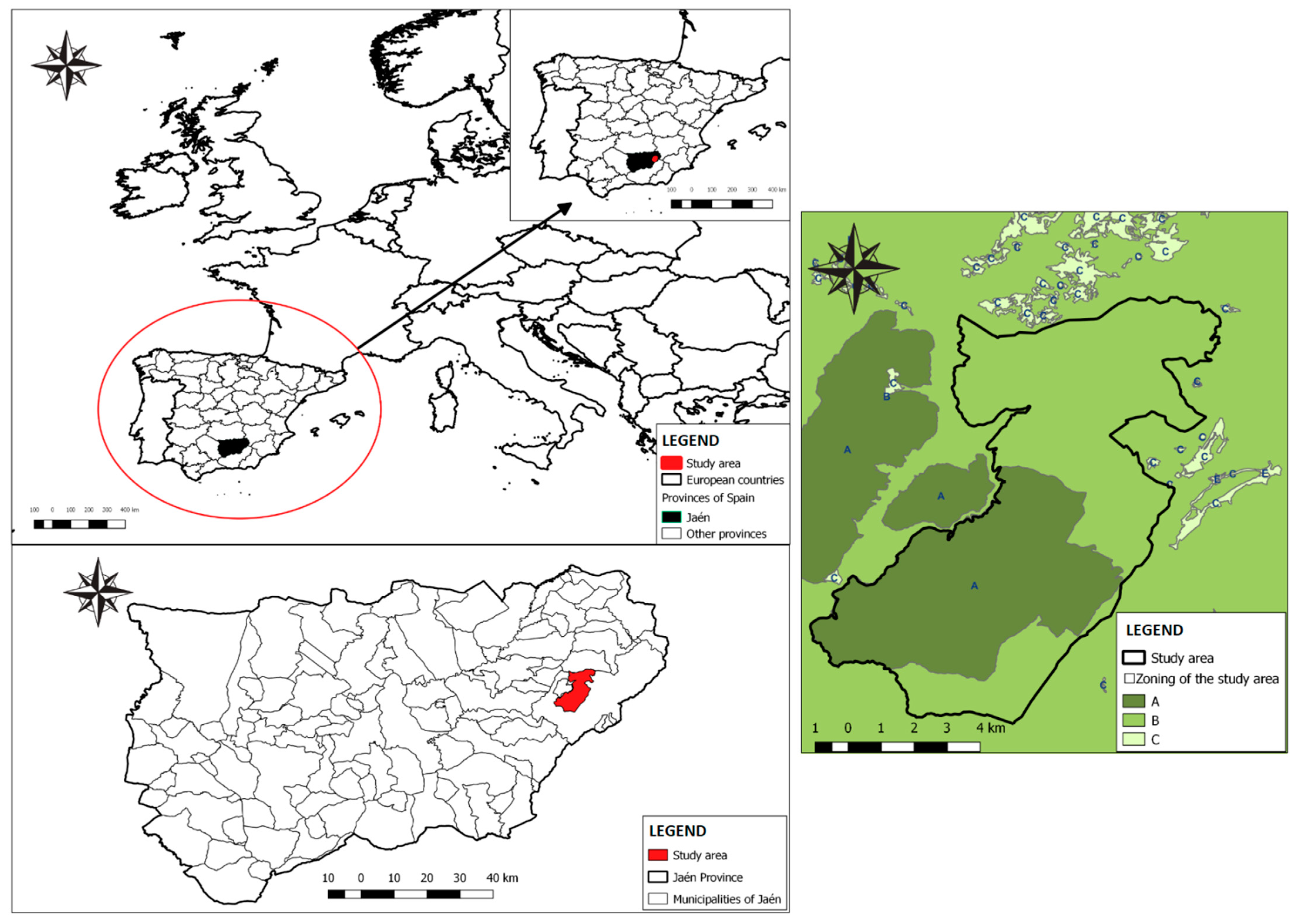
The selected study area is located in the Sierra de Cazorla, Segura, and Las Villas Natural Park (Southeastern Spain) (Figure 1). It is a public forest area of 9675 ha and includes the following mountains: ‘Cerro de las Canasteras, JA-10027-JA’, ‘Desde Aguamulas hasta el Arroyo de las Espumaredas, JA-10028-JA’, ‘Malezas de Pontones, JA-10029-JA’, ‘Montalvo y Hoya Morena, JA-10030-JA’, ‘Peña Amusgo hasta el Arroyo de las Espumaredas, JA-10031-JA’, ‘San Román, JA-10072-JA’, ‘Fuente del Roble, JA-10074-JA’, ‘Las Ánimas y Mirabuenos, JA-10125-JA’, ‘Los Goldines, JA-10205-JA’, and the expropriation ‘Entre Montalvo y Los Goldines’.

The Sierra de Cazorla, Segura, and Las Villas Natural Park is the largest protected area in Spain and the second largest in Europe [19], with an approximate surface area of 210,000 ha, and its administrative surface area is spread over 23 municipalities [20]. Santiago-Pontones stands out, as 33% of the protected area belongs to this municipality. The management of this forest has been mainly focused on protection, as part of the surface area (4106 ha) is located in zone A, a reserve zone (Figure 1), of the Natural Resources Management Plan, whose main objective is the conservation of protected species, both flora and fauna.

The area is dominated by stands of the genus Pinus, the most representative being Pinus halepensis Mill., with mixed stands of this species and Pinus pinaster Ait. in the north of the mountain, as well as pure stands of the latter species. The altitude ranges from 640 m above sea level (around the shores of the Tranco reservoir) to 1760 m. According to the Management Project, the average slope is very steep, with 62% of the surface area having a slope greater than 35%. A Mediterranean climate prevails, though with colder and rainier winters than average. Given the conditions of this climate, the fire register occupies large areas of the forest. However, no fire has occurred in the study area since 1968 according to available records, although there have been large forest fires in nearby areas such as ‘Puerto de las Palomas’ in 2001 (863 ha), ‘Embalse del Tranco’ in 2005 (5116 ha) (with some spotting fires that affected the study area but did not prosper due to the prompt response of the fire service), and ‘Segura de la Sierra’ in 2017 (686 ha) [21]. In the area close to the Natural Park, the ‘Quesada’ fire occurred in 2015 (9806 ha). These events had the spread of crown fires in common. The generation of fuel model mapping is therefore of great importance, and LiDAR technology offers significant advantages for the determination of the models.

2.2. Definition of Fuel Models

In this study, the UCO40 fuel models (a description of is shown in the Appendix A) [22], which are based on the categorisations made by [23], were utilised. The models were divided into six fuel model groups: grass (P), grass scrubs (PM), scrub (M), litter grass scrub (HPM), litter slash (HR), and slash (R). Based on information from previous authors [8,18,21], some UCO40 fuel model characteristics had been defined, namely vegetation type, plant taxa, and vegetation position and structure. The first four characteristics were defined with open access cartography, itineraries, and LiDAR (

Table 1. Open source information and the defined vegetation characteristics.

Information	Cartography	Itineraries	LiDAR
Vegetation type	X		X
Life form	X		X
Plant taxa	X	X
Position	X		X

). This allowed us to divide the area into smaller zones and make the computer processing faster because the processing of this information for all study areas at once was impossible.

The used open access cartography was from the Information System on Land Occupation of Spain (SIOSE) [23] that uses the photointerpretation of various types of images to define the polygons of the types of vegetation. SIOSE provides information of the spatial distribution of different types of vegetation, as well as the cover of trees, scrubs, and plants taxa. The used itineraries were the National Forest Itinerary (INF) [24] and the itinerary realised in the Resource Management Project of the area; their use with SIOSE allowed us to know whether the information about the plant taxa was correct and correct it if necessary. LiDAR was used to confirm the location, position, and type of vegetation. However, it was primarily used to obtain the structure and cover of the vegetation.

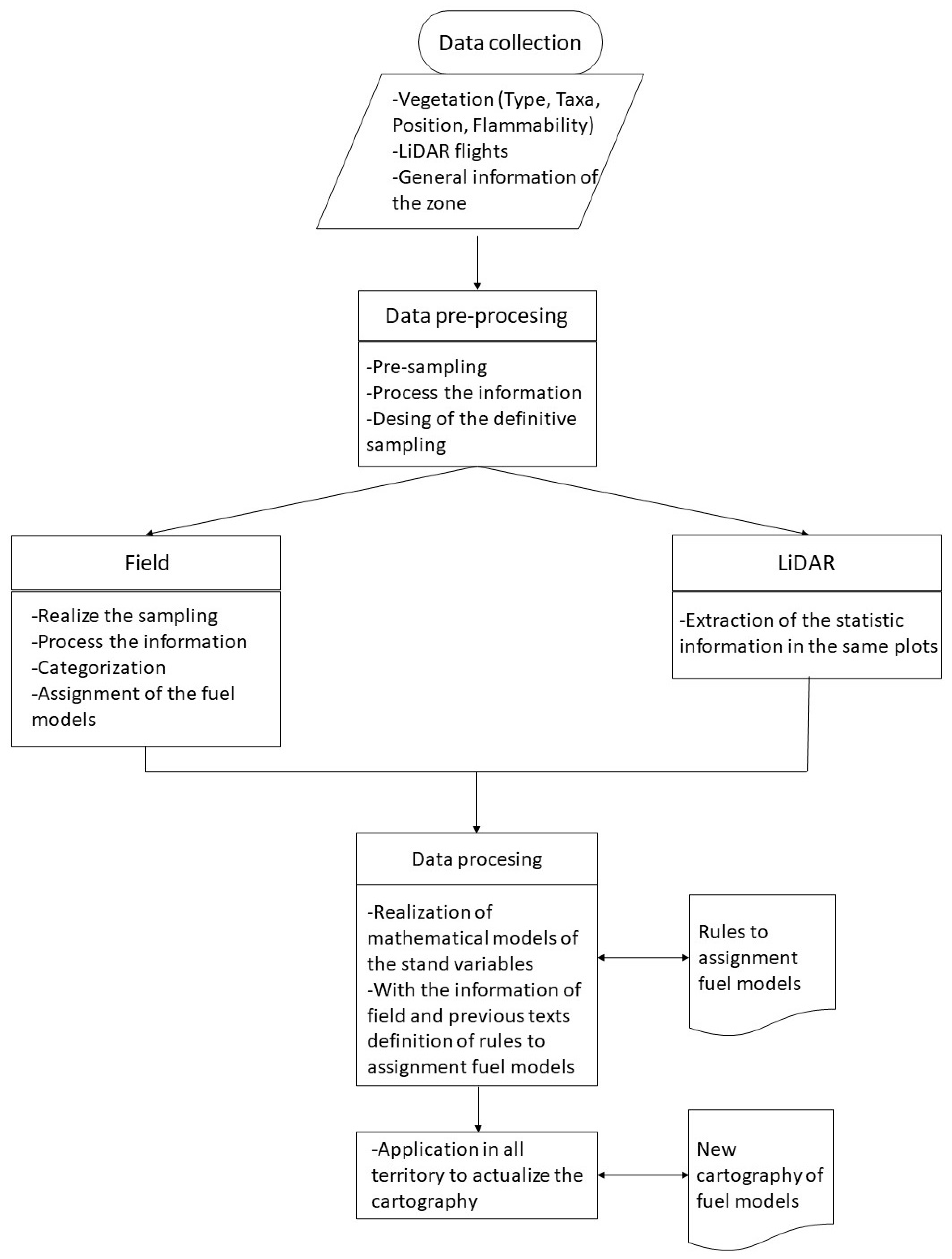
This information not only allowed us to define better the areas of each fuel model but also helped us characterise the study area. Our workflow is shown in Figure 2.

The objective of the determination of the fuel models was to assign a fuel load to evaluate the suppression difficulty index [18,25]. This variable is necessary to determine the energy behaviour sub-index that can be used calculate surface, crown, and eruptive fires.

2.3. Design of Sample Plots for Model Characterisation

In the study area, P, PM, and M areas are scarce and large fires have a tendency to occur in forest systems dominated by a tree stratum in the vicinity of the area. Thus, in this study, we focused on the groups of woody fuels, namely HPM and HR.

We conducted a simple random pre-sampling of 12 circular plots with a radius of 20 m, with an overall surface area of 1256.64 m² each one. The field variables were evaluated by different tools. A TOPCON GMS-2 GPS was used to determinate the centre points of the plots where the data were recollected. A Hypsometer Vertex IV was used to find the heights of the trees, base canopies, and crowns. A Pi tape was used to measure the normal crown diameter, and a metric tape was used to define the plots limits, crown diameters, and scrub heights. The tree and scrub canopy covers were measured and then assigned a number from 1 to 4, with 1 representing the range between 0 and 25%, 2 representing the range between >25 and 50%, 3 representing the range between >50 and 75%, and 4 representing the range between 75 and 100%.

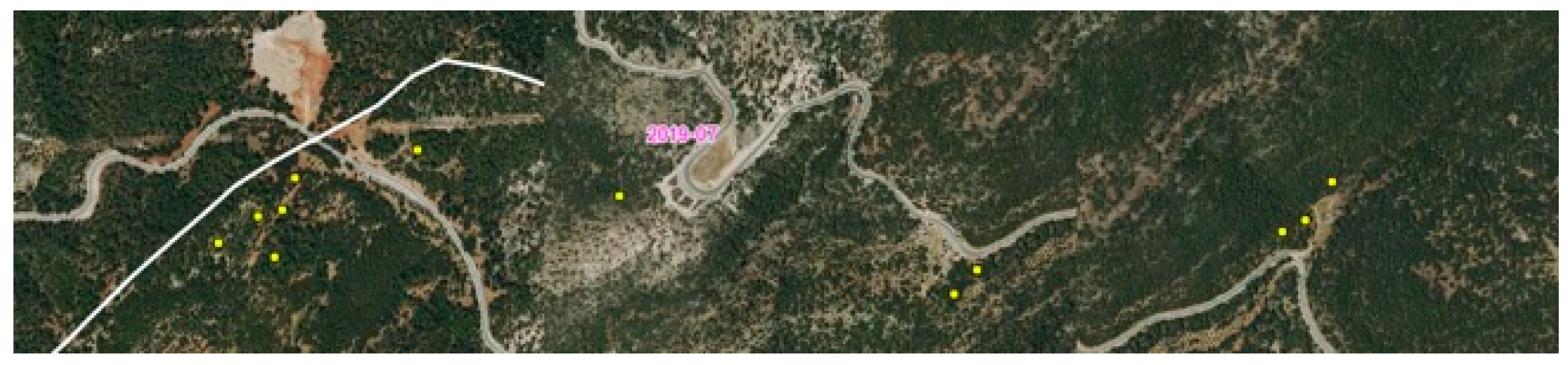
The plots were collected at the points shown in Figure 3.

The predominant species was Pinus pinaster; the variables that were measured in field were normal diameter, crown height, crown diameter with two measurements, height, age, species and fraction of tree and shrub canopy cover, mean shrub height, and the species comprising that stratum. Data were collected for each individual tree in the plot to calculate the density of trees. This pre-sample was done to understand the variability of the forest stand. Knowing the density of trees in these 12 plots, a statistics study was conducted to determine the number of plots necessary to reach a 90% (accuracy) of fiducial probability. With this, we avoided making more or less plots than necessary, so costs were optimised. Furthermore, this allowed us to obtain errors within our margins and guaranteed that the next static analyses were based on a reliable source.

The statistical study was carried out to determine the number of total plots necessary to comply with the 90% confidence probability; the number was found to be 28 plots.

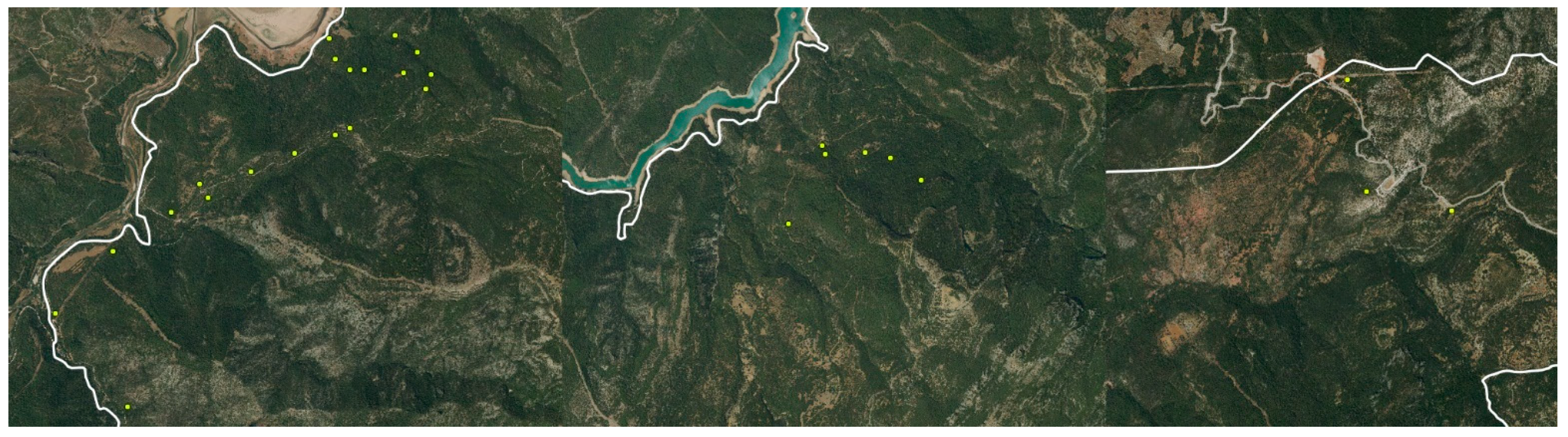
The 28 circular plots did not contain all 12 pre-sampling plots because these were located in the north of the forest and the general inventory preferred simple random sampling throughout the area (Figure 4).

The distribution of the sampling points was not homogeneous because the road network is scarce and, as mentioned above, the average gradient is very steep, which makes it impossible to carry out inventories at great distances from established routes. Data on diameter at breast height, height, height at the crown base, and species were collected for each stand in the sample plots. In addition, the following data were collected: fraction of tree and shrub canopy cover, mean shrub height, and the species comprising that stratum. The crown weight (kg) of the tree stratum in the plots was estimated by using existing data on the crown weight (branches > 7 cm, 2–7 cm, <2 cm, and leaves) of species present in the sample plots, as well as other collected information [26].

2.4. LiDAR Data

The LiDAR data of the area were acquired in 2017 at the Download Centre of the National Centre for Geographic Information (CNIG) of the Ministry of Transport, Mobility, and Urban Agenda within the PNOA program. These data were captured in 2014 with a LEICA ALS60 laser scanner (airborne laser scanner), and the points had an average density of 0.5 points/m² within an area of 2 km × 2 km. The LAZ files had to be decompressed for us to use the LAS with the LASzip application [27]. Data processing was carried out using the LiDAR FUSION pulse interpretation software [28] from the Remote Sensing Applications Centre (USDA), which was necessary for the statistical information processing of the laser pulses information.

For separating ground and vegetation, it was necessary to use the GroundFilter command. The command was designed to eliminate returns that do not represent reality and to separate ground and non-ground points. It was especially tested in high-density flights (4 puntos/m²), but its designers indicated in the case of low-density flights, it is necessary to test different coefficients that are applied in the command. Our tests showed that the default values in this command were the best fit for our area and reality, as other values produced a higher number of off-average points.

The height used to differentiate the tree layer from the understory was 2.5 m. To match the field information with the LiDAR data, the same areas and centre points of the 28 plots that were found were used for the stand measurement of tree mass, and seventy-eight variables in total were obtained from the LiDAR information for each plot using the CloudMetrics command.

2.5. Modelling of Dasometric Variables

It was necessary to use a combination of the data collected in the field plots and the LiDAR information under to generate predictive models using the dasometric variables of the stand. Firstly, we studied the composition of the Pinus spp. and Quercus spp. genera; subsequently, only the dominant genus was studied. The studied dependent variables included mean height (m), crown base height (m), basal area (m²/ha), mean normal diameter (cm), understory height (m), base canopy height (m), and Z-height (m).

The models were built to have a high predictive power by avoiding the redundancy of variables and greater collinearity according to Spearman. By performing a Shapiro normality test, it was observed that the variables were not normally distributed, so the natural logarithm of each variable was used to normalise the data. The criteria for building the models were a high predictive power and avoidance of collinearity. Each variable was significant at <0.05. For the choice of model, different variable combinations were tested to generate different models, and then the best one was selected.

2.6. Actualisation of the Fuel Model Cartography

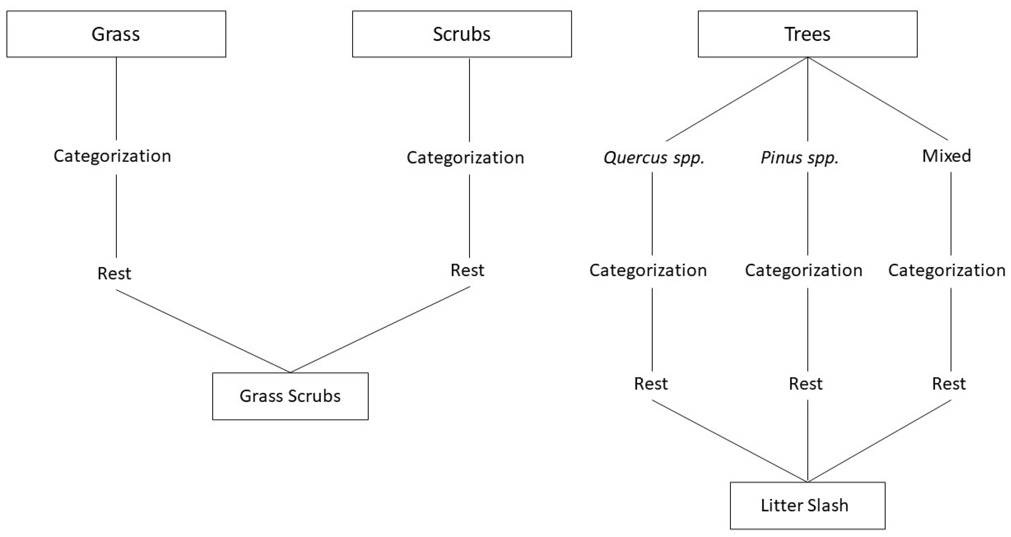
The information of vegetation type, life form, position, and plant taxa allowed us to de-fine 3 big zones in our study area: Grass, Scrubs, and Trees. With the rules shown in the Appendix B (

Table A1. Description of the UCO40 fuel models and the supporting variables assigned to them.

Models	Fcca (%) 1	Fccm (%) 2	Tree Height (m)	Scrub Height (m)	Grass Height (m)	Weight of Tree Crowns (kg)	Observations 3
P1	<10	<10	-	-	0–0.3	-	Summits
P2	<10	<10	-	-	0–0.3	-	Dehesas
P3	<10	<10	-	-	0.3–0.6	-	Reforestations
P4	<10	<10	-	-	0.3–0.6	-	Dehesas
P5	<10	<10	-	-	0.6–0.9	-	Natural grasslands or Post-fire areas
P6	<10	<10	-	-	0.6–0.9	-	Post-fire areas
P7	<10	<10	-	-	0.9–1.2	-	Abandoned crops
P8	<10	<10	-	-	0.9–1.2	-	Riverbanks
P9	<10	<10	-	-	1.2–2.5	-	Reedbeds
PM1	<25	<25	-	0.3–0.6		-	Discontinuity
PM2	<25	<25	-	0.6–1.2		-	Discontinuity
PM3	<25	>25	-	0.3–0.6		-	Continuity
PM4	<25	>25	-	0.6–1.2		-	Continuity
M1	<10	>50	-	0–0.6		-	Discontinuity
M2	<10	>50	-	0–0.6		-	Continuity
M3	<10	>50	-	0.6–1.5		-	Continuity
M4	<50	>50	-	0.6–1.5		-	Continuity
M5	<50	>50	<7	-	-	-	Latizal
M6	<10	>50	-	0.6–1.5	-	-	Discontinuity
M7	<50	>50	<7	-	-	-	High scrub
M8	<50	>50	-	0.6–1.5	-	-	Continuity
M9	<10	>50	-	1.5–2.5	-	-	Two strata
HPM1	>50	>25	>7	<0.3	-	-	Conifers
HPM2	>50	>25	<7	<0.3	-	-	Hardwood
HPM3	>50	>25	>7	0.3–0.9	-	-	Eucalyptus stands
HPM4	>50	>25	>7	0.3–0.9	-	-	Conifers
HPM5	>50	>25	<7	>0.9	-	-	Reforestation without treatment
HR1	>75	<10	>7	-	-	>12.78	Post-fire areas
HR2	>75	<10	>7	-	-	>25.56	Hardwood
HR3	>75	<10	>7	-	-	>38.34	Conifers
HR4	>75	<10	>7	-	-	>51.12	Hardwood
HR5	>75	<10	>7	-	-	>63.90	Conifers
HR6	>75	<10	>7	-	-	>76.68	Conifers
HR7	>75	<10	>7	-	-	>89.46	Mixed
HR8	>75	<10	>7	-	-	>102.24	Conifers
HR9	>75	<10	>7	-	-	>115.02	Eucalyptus stands

¹ Fcca: tree canopy cover; ² Fccm: scrubs canopy cover; ³ Observations: the most likely locations where these models are located, their distribution, and divisions of the vegetation stratum.

), the 3 zones were defined as small polygons of each type of fuel model, but there were zones not defined in any fuel model, as can be observed in Figure 5. The areas not defined as Grass and Scrub fuel models were defined as Grass Scrub models. The Trees zone was divided into 3 types—Quercus spp., Pinus spp., and mixed—that were again divided by the rules, but the areas with a low canopy cover of scrubs were defined as Litter Slash.

It has not been possible to classify Litter fuel because it does not exist in the area. This is because there are no forest extraction activities that produce this type of fuel, as the main goal of management is to protect endangered species.

3. Results

From the density of trees obtained in the pre-sampling plots, the definitive number of plots was defined. A summary of the data obtained in the pre-sampling step is presented in

Table 2. Summary of data obtained in the pre-sampling plots (N = 12).

Variable	Maximum	Minimum	Average	Standard Deviation
Normal diameter (m)	56.8	19.50	37.01	10.39
Height (m)	27.6	8.90	123.50	4.7
Crown height (m)	12.10	3.5	7.32	2.34
Diameter of crown (m)	10.5	3.31	6.39	2.05
Age (years)	100	30	65.7	25.06
Number of trees	30	10	18.42	5.77

. In order to obtain the results shown in

Table 3. Summary of data obtained in the field sample plots (N = 28).

Variable	Maximum	Minimum	Average	Standard Deviation
Normal diameter (m)	46.8	12.65	27.97	7.66
Height (m)	20.95	6.45	13.37	3.63
Base canopy height (m)	11.35	1.89	6.35	2.42
Tree density (trees/ha)	915.14	36.06	413.38	231.15
Basal area (m2/ha)	62.68	9.89	26.89	11.69
Scrub height (m)	1.8	0.1	0.77	0.49

, the 28 sample plots were evaluated. The difference between the maximum and minimum of the tree density could have resulted in a large sampling error, but one of the advantages of making pre-sampling plots is minimizing errors. The error obtained for the sampling was 3.14%.

The results of

Table 4. Models and evaluation of models for stand variables with Pinus and Quercus genera.

Variable	Model	Parameter	Estimation	Standard Error	R2
Mean height	Ln Hm 1 = a + a1 × Ln E.P99 2 + a2 × Ln I.CV 3	a a1 a2	0.7091 0.7458 −0.4853	0.1952	0.4393
Base canopy height	Ln HBC 4 = a + a1 × Ln E. máx. 5 + a2 × Ln I.P1 6	a a1 a2	−0.5335 0.9890 0.2589	0.193	0.5973
Basal area	Ln G 7 = a + a1 × Ln E.L4 8 + a2 × Ln 1st R.M. 9 + a3 × Ln P.A. 10	a a1 a2 a3	−4.5006 1.1178 −0.4970 4.0681	0.8448	0.6623
Mean normal diameter	Ln ø 11 = a + a1 × Ln E.mod. 12 + a2 × Ln T.R.mod. 13	a a1 a2	0.9358 0.4592 0.5626	0.2073	0.6001
Scrub height	Ln Hmat. 14 = a + a1 × Ln E. MAD 15 mode + a2 × Ln I. min. 16 + a3 × Ln 2nd R.E.2.5 17	a a1 a2 a3	−8.3944 1.3001 4.2334 0.4808	0.5307	0.5846
Weight of tree crowns	Ln Weight crowns 18 = a + a1 × Ln T.R.mod. + a2 × Ln I.L3 19 + a3 × Ln %1st R.Mode 20 + a4 × Ln %T.R.mod 21	a a1 a2 a3	4.7816 −0.2616 0.0445 −55.07673	0.2156	0.7331

¹ Hm: mean height; ² E.P99: 99th percentile of elevation; ³ I.CV: coefficient of variation of intensity; ⁴ HBC: base canopy height; ⁵ E. max: maximum elevation; ⁶ I.P1: first percentile of intensity; ⁷ G: basal area; ⁸ E.L4: L4 moment of elevation; ⁹ 1st R.M.: first returns above median; ¹⁰ P.A.: area profile; ¹¹ Ø: mean normal diameter; ¹² E. mod.: mode of the elevation; ¹³ T.R.mod: all returns above the mode (total of the first returns); ¹⁴ Hmat: scrub height; ¹⁵ E. MAD mode: mode of absolute deviation of median elevation; ¹⁶ I. min: minimum intensity; ¹⁷ 2nd R.E.2.5: second returns above median; ¹⁸ Weight crowns: weight of tree crowns; ¹⁹ I.L3: L3 moment of intensity; ²⁰ %1st R.Mode: percentage of first returns above the mode; ²¹ T.R.mod: percentage of all returns above the mode (total of the first returns).

were derived from the statistical study of the Pinus spp. and Quercus spp. genera. In view of the results obtained in Table 4, it was decided to conduct a statistical study of those variables for which the model did not obtain the most appropriate results. In this case, this meant studying the dominant pine genus. The prediction of the distance between the base of the crowns and the understory (m) was also analysed (

Table 5. Models and model evaluation for Pinus spp. stand variables.

Variable	Model	Parameter	Estimation	Standard Error	R2
Mean height	Ln Hm = a + a1 × Ln I. kurtosis 1 + a2 × Ln % T.R.M. 2	a a1 a2	0.9703 −0.1619 0.6587	0.1587	0.8201
Base canopy height	Ln HBC = a + a1 × Ln E.L. kurtosis 3 + a2 × Ln % T.R.M.	a a1 a2	0.9348 0.3393 0.6747	0.1985	0.8224
Z-height	Ln H.Z. 4 = a + a1 × Ln E. L4 + a2 × Ln %1st R.M. 5	a a1 a2	0.4188 0.3471 0.7951	0.1983	0.8677

¹ I. kurtosis: intensity of kurtosis; ² % T.R.M.: percentage of all returns above mean; ³ E.L. kurtosis: logarithm of kurtosis elevation; ⁴ H.Z.: Z-height, height between canopy base and scrubs; ⁵ %1st R.M.: percentage of first returns above the mean.

).

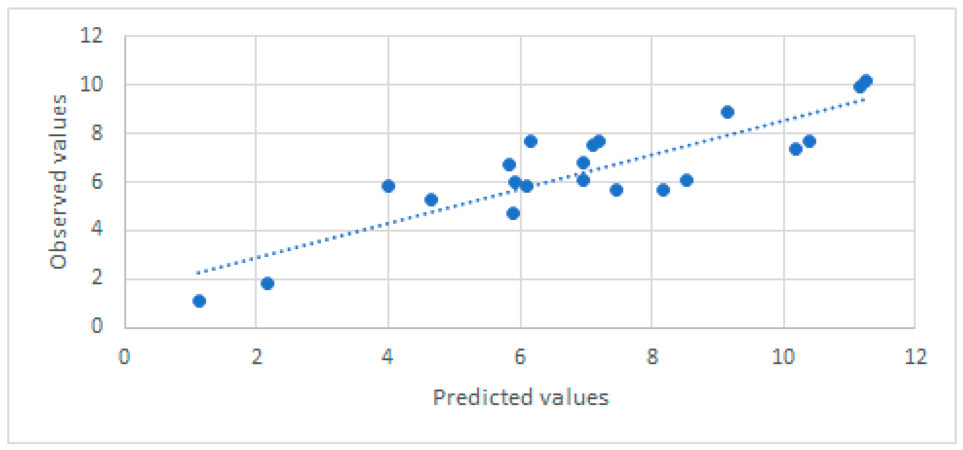
The coefficients of the models for the stand characteristics ranged from 0.4393 for mean height to 0.8677 for Z-height (Table 4 and Table 5), and the predicted values were similar to those observed in most cases (Figure 6). In the values of the joint data of the Pinus spp. and Quercus spp. genera present in the sampling plots, it can be seen the models did not yield high R² values. As such, statistical analysis was again conducted for each of the genera, and obtained better determination coefficients for the dominant genus Pinus. The mean height model had a coefficient of determination of between 0.4393 and 0.8201 (Table 5).

The rules defined for classifying forest areas into fuel patterns (Appendix B) are mainly based on tree and scrub cover, as well as the height of the tree, scrub, or grassland. These characteristics are sufficient to differentiate between models associated with grass, grass scrub, shrub, and litter grass scrub, but they made it difficult to differentiate between the litter grass scrub model group and the litter slash group. For this reason, the canopy weight variable was included in the rules because the higher the canopy weight, the greater the litter layer under the canopy.

The proposed methodology was found to be 39.28% correct in terms of characterising individual models (

Table 6. Predicted (based on the rules set in Table 6) and observed fuel models for the 28 inventory plots.

Plot	Observed Model	Predicted Model
1	HPM4	HPM4
2	M4	M4
3	HPM5	HPM5
4	HR4	HPM4
5	HR4	HR4
6	HR6	HR1
7	HR3	HR1
8	HR7	HR2
9	HR7	HR1
10	HR4	M7
11	HPM4	HPM4
12	HPM5	HPM5
13	HR7	HR1
14	M7	HPM5
15	M4	HPM4
16	HR4	HR1
17	HPM4	HPM4
18	HPM5	HPM4
19	HR7	HR4
20	HR3	HPM4
21	HPM4	HPM4
22	M9	HR1
23	HPM4	HR1
24	M7	HR2
25	HR3	HPM5
26	HPM4	HPM4
27	HPM4	HPM4
28	HPM4	HPM4

). When the models were grouped into clusters, the correct assignment strongly increased the prediction in the tree stand (90.9% and 72.73%) compared to the shrublands (40%) (

Table 7. Groups of predicted (based on the rules in Appendix B) and observed fuel models for the 28 inventory plots, as well as the precision of the estimation.

Predicted Model
Observed Model	Scrubs	Litter Grass Scrub	Litter Slash	Accuracy by Model Group (%)
Scrubs	1	1	1	40
Litter Grass Scrub	0	10	1	90.90
Litter Slash	1	3	8	72.73

).

4. Discussion

The use of the PNOA LiDAR to estimate stand variables has some limitations [29,30]. As can be seen, the mean height and height at the base of the canopy did not yield good fits, although the variables were significant. Similar results were observed for other parameters, such as basal area, normal diameter, and understory height. This was because the density of pulses was low, so it was difficult for a high number of pulses to penetrate the tree canopy and provide information on the vegetation below the canopy. In the area under study, the canopy usually has no gaps, and it is possible that in more open areas, such as a dehesa, the study of the stand characteristics with the PNOA LiDAR information would yield better results [31]. To confirm this assumption, the same statistical study was carried out using the stand characteristics while differentiating them by genus, and we obtained the results shown in Table 5 for pine stands. The results obtained for Quercus spp. are not shown in detail because their abundance was low and only generated noise. The low density of pulses made it difficult to obtain information in stands with two strata where one is dominated by the other.

The resulting models have shown strong quality compared to those of other studies in which statistical analysis was performed using LiDAR data with a higher density of points, such as the one developed in [32], in which the density was more than 4 pulses/m² with an R² of 0.63 for the basal area variable. The results obtained in the characterisation of the fuel models at the individual and group levels indicated that in most cases, the predicted individual model was associated with another nearby model within the same group, so it is necessary its adjust for future use. The number of times a litterfall residual model was confounded with a scrub grass litterfall model is relatively high, so it would be appropriate to study these specific cases to know the fit of the variables or even to add some new ones. The precision of the scrub group was low and confused with the groups associated with trees because they were vertically distributed at the same level as Quercus spp., in addition to the fact that there were no large areas in which only scrub could be found, as can be seen in the number of plots that this group had compared to the rest of the groups. Therefore, it would be a good idea in the future to include basal area variable in order to be able to better discern in which cases this is sufficiently high enough to be considered a limiting factor for differentiation. Another possibility is that actions were carried out between the flight and the field visit, so the structure obtained with LiDAR did not represent reality and, therefore, the predicted model.

The results obtained in this work had close relationships with the vegetation cover of the pilot area defined for the development of the methodology. In the sampled area, shrub, grassland, and slash models were found to have a low presence. In order to increase the precision of the developed algorithms, the methodology is being applied in other protected areas of the natural park where the representativeness of these groups of fuel models is greater. This activity will allow us to evaluate the predictive capacity of the algorithms and facilitate their applicability to other forest landscapes.

The improvement in the methodology used has been substantial, as it allows for the accurate updating of an area with a minimum need for field visits. This update of the coverage used in fuel models implies improvements in the optimisation of prevention by allowing researchers to carry out simulations of potential fires with greater precision. The best adjustment in the identification and characterisation of fuel models through the developed LiDAR methodology will help to increase the quality and accuracy of the prioritisation indices of defence actions against forest fires. In this sense, indices that evaluate the potential fire behaviour (PFBI), the energetic release component of fire propagation (Ice), and extinction difficulty (SDI) calculated based on a better quality of forest fuel maps can decrease uncertainty in decision making.

These indices will also help to optimize firefighting tasks, since forest fires will be less likely to behave in an unexpected way (Figure 7).

5. Conclusions

The purpose of this study was to provide an accessible tool for forest managers and emergency directors to characterise fuel models of their territories. In principle, it was necessary to obtain models of the stand variables that constitute the forest mass, for which the collection of field data was required. We performed statistical analyses of the dataset prepared for the homogeneous stand existing in the forest. Following the first obtained results, the decision was made to conduct statistical analysis for the dominant stratum of the stand. This clarified the capability of low-density LiDAR in mixed stands.

From the generated models for the stand characteristics and the analysis, it was possible to generate rules that allowed for the generation of coverage of the UCO40 fuel models on any area traversed with airborne LiDAR. The performed characterisation showed that there was a high capacity to hit the fuel model group on tree-covered surfaces. The same cannot be said for areas covered by scrubs, as the area under study had very few of such areas; therefore, their characterisation was not optimised.

This methodology is useful for estimating the forest stand structure present in the territory, as well as improving and updating its cartography. This tool has been made available to emergency managers and administrators, streamlining decision making by being fastand update. Especially in areas that are difficult to access and where, under normal conditions, it would be impossible to assess their characteristics. Through this study, a set of algorithms were obtained to calculate different stand variables with airborne LiDAR, such as mean height, crown base height, basal area, normal mean diameter, shrub height, crown weight, and Z-height.

The high predictive capacity of the developed models is a guarantee of quality for applications in protected surfaces with access restrictions to collect field information. Likewise, the flow chart of the methodology and the division of the surface into groups with different types of vegetation provide an application guide in other territories. This advantage provides solutions to managers with responsibilities in the prevention and extinction of forest fires.

The results of this study show that the generated information related to combustibility has a high level of adjustment. This quality affects the characterisation of indices that predict the energy behaviour of fires. These indices improve the ability to predict suppression opportunities in operational scenarios, assisting managers in planning activities for fire defence in forest landscapes.

Another consequence of this study is our reduction of uncertainty by using an updated and high precision fuel model mapping. With the results obtained in this study, it is possible to identify areas that are optimal for extinguishing forest fires and to locate areas that can be adapted for use and that do not have safety conditions for firefighters to carry out suppression activities. These tools will undoubtedly increase the safety of suppression operations and reduce uncertainty.

References

- North, M.P.; Stephens, S.L.; Collins, B.M.; Agee, J.K.; Aplet, G.; Franklin, J.F.; Fulé, P.Z. Reform forest fire management. Science 2015, 349, 1280–1281. [Google Scholar] [CrossRef] [PubMed]
- Jaffe, D.; Hafner, W.; Chand, D.; Westerling, A.; Spracklen, D. Interannual variations in PM2. 5 due to wildfires in the Western United States. Environ. Sci. Technol. 2008, 42, 2812–2818. [Google Scholar] [CrossRef] [PubMed]
- Piñol, J.; Terradas, J.; Lloret, F. Climate warming, wildfire hazard, and wildfire occurrence in coastal eastern Spain. Clim. Chang. 1998, 38, 345–357. [Google Scholar] [CrossRef]
- Abrha, H.; Adhana, K. Desa’A national forest reserve susceptibility to fire under climate change. For. Sci. Technol. 2019, 15, 140–146. [Google Scholar] [CrossRef]
- Molina, J.R.; González-Cabán, A.; Silva, F.R. Wildfires impact on the economic susceptibility of recreation activities: Application in a Mediterranean protected area. J. Environ. Manag. 2019, 245, 454–463. [Google Scholar] [CrossRef] [PubMed]
- Hoover, T. Disequilibrium: Wildfires, the Fire Triangle, and CO2 Extinguishers. Sci. Scope 2017, 41. [Google Scholar] [CrossRef]
- Robles, A.M.; Agudo, G.J. El Sistema de Información Meteorológica del Plan de Emergencias por Incendios Forestales de Andalucía (Andalucía, España) Plan INFOCA. In Proceedings of the 4th International Wildland Fire Conference, Seville, Spain, 13–17 May 2007. [Google Scholar]
- Anderson, H.E. Aids to Determining Fuel Models for Estimating Fire Behavior; USDA Forest Service: Boise, ID, USA, 1982. [Google Scholar]
- Graham, R.T.; McCaffrey, S.; Jain, T.B. Science Basis for Changing Forest Structure to Modify Wildfire Behavior and Severity; United States Department of Agriculture Forest Service, Rocky Mountain Research Station: Fort Collins, CO, USA, 2004. [Google Scholar]
- Finney, M.A.; Seli, R.C.; McHugh, C.W.; Ager, A.A.; Bahro, B.; Agee, J.K. Simulation of long-term landscape-level fuel treatment effects on large wildfires. Int. J. Wildland Fire 2007, 16, 712–727. [Google Scholar] [CrossRef] [Green Version]
- Ottmar, R.D.; Hudak, A.T.; Prichard, S.J.; Wright, C.S.; Restaino, J.; Kennedy, M.C.; Vihnanek, R.E. Pre- and post-fire surface fuel and cover measurements collected in the southeastern United States for model evaluation and development—RxCADRE 2008, 2011, and 2012. Int. J. Wildland Fire 2016, 25, 10–24. [Google Scholar] [CrossRef]
- Agee, J.K.; Bahro, B.; Finney, M.A.; Omi, P.N.; Sapsis, D.B.; Skinner, C.N.; van Wagtendonk, J.W.; Weatherspoon, C.P. The use of shaded fuelbreaks in landscape fire management. For. Ecol. Manag. 2000, 127, 56–66. [Google Scholar] [CrossRef]
- Wang, X.; Pan, H.Z.; Guo, K.; Yang, X.; Luo, S. The evolution of LiDAR and its application in high precision measurement. In Proceedings of the IOP Conference Series: Earth and Environmental Science, Changchun, China, 1–14 October 2020. [Google Scholar]
- Dubayah, R.; Drake, J. Lidar Remote Sensing for Forestry. J. For. 1999, 98, 44–46. [Google Scholar]
- Mutlu, M.; Popescu, S.C.; Stripling, C.; Spencer, T. Mapping surface fuel models using lidar and multispectral data fusion for fire behavior. Remote Sens. Environ. 2008, 112, 274–285. [Google Scholar] [CrossRef]
- Moran, C.; Kane, V.; Seielstad, C. Mapping Forest Canopy Fuels in the Western United States with LiDAR—Landsat Covariance. Remote Sens. 2020, 12, 1000. [Google Scholar] [CrossRef] [Green Version]
- Cruz, M.G.; Alexander, M.E.; Wakimoto, R.H. Modeling the Likelihood of Crown Fire Occurrence in Conifer Forest Stands. For. Sci. 2004, 50, 640–658. [Google Scholar]
- Rodríguez y Silva, F.; O’Connor, C.D.; Thompson, M.P.; Molina, J.R.; Calkin, D.E. Modelling suppression difficulty: Current and future applications. Int. J. Wildland Fire 2020, 29, 739–751. [Google Scholar] [CrossRef]
- Junta de Andalucía. Parque Natural Sierra de Cazorla, Segura y Las Villas. Available online: http://www.juntadeandalucia.es/medioambiente/site/portalweb/menuitem.220de8226575045b25f09a105510e1ca/?vgnextoid=8ac0ee9b421f4310VgnVCM2000000624e50aRCRD (accessed on 1 July 2021).
- Decreto 191/2017, de 28 de noviembre, por el que se declara la zona especial de conservación Sierras de Cazorla, Segura y Las Villas (ES0000035) y se aprueban el Plan de Ordenación de los Recursos Naturales y el Plan Rector de Uso y Gestión del Parque Natural Sierras de Cazorla, Segura y Las Villas. Available online: https://noticias.juridicas.com/base_datos/CCAA/611143-d-191-2017-de-28-nov-ca-andalucia-declara-zona-especial-de-conservacion.html (accessed on 28 December 2017).
- Rodríguez y Silva, F.; Molina, J.R. Manual Técnico Para la Modelización de la Combustibilidad Asociada a los Ecosistemas Forestales Mediterráneos; Laboratorio de Defensa contra Incendios Forestales, Departamento de Ingeniería Forestal, Universidad de Córdoba: Cordoba, Spain, 2010. [Google Scholar]
- Scott, J.H.; Burgan, R.E. Standard Fire Behaviour Fuel Model: A Comprehensive Set for Use with Rothermel’s Surface Fire Spread Model; USDA Forest Service: Boise, ID, USA, 2005. [Google Scholar]
- Ministerio de Fomento. Sistema de Información de Ocupación del Suelo en España. Available online: https://www.siose.es/web/guest/productos (accessed on 13 July 2021).
- Ministerio para la Transición Ecológica y el reto Demográfico. Tercer Inventario Forestal Nacional. Available online: https://www.miteco.gob.es/es/biodiversidad/servicios/banco-datos-naturaleza/informacion-disponible/ifn3.aspx (accessed on 13 July 2021).
- Rodríguez y Silva, F.; Molina, J.R.; González-Cabán, A. A methodology for determining operational priorities for prevention and suppression of wildland fires. Int. J. Wildland Fire 2014, 23, 544–554. [Google Scholar] [CrossRef]
- Agudo Romero, R.; Muñoz Martínez, M.; del Pino del Castillo, O. Primer Inventario De Sumideros De CO2 De Andalucía; Junta de Andalucía: Sevilla, Spain, 2007. [Google Scholar]
- Isenburg, M. LASzip: Lossless compression of LiDAR data. Photogramm. Eng. Remote Sens. 2011, 79, 209–217. [Google Scholar] [CrossRef]
- McGaughey, R.; Forester, R.; Carson, W. Fusing LIDAR data, photographs, and other data using 2D and 3Dvisualization techniques. Proc. Terrain Data Appl. Vis. Connect. 2003, 28, 16–24. [Google Scholar]
- Hadaś, E.; Estornell, J. Accuracy of tree geometric parameters depending on the LiDAR data density. Eur. J. Remote Sens. 2016, 49, 73–92. [Google Scholar] [CrossRef] [Green Version]
- Marino, E.; Tomé, J.; Madrigal, J.; Hernando, C. Effect of LiDAR pulse density on crown fuel modelling, (Fuels of Today—Fire Behavior of Tomorrow). In Proceedings of the 6th International Fire Behavior and Fuels Conference, Marseille, France, 29 April–3 May 2019. [Google Scholar]
- Borlaf, I.; Tanase, M.; Sal, A. Methods for tree cover extraction from high resolution orthophotos and airborne LiDAR scanning in Spanish dehesas. Rev. Teledetec. 2019, 53, 17–32. [Google Scholar] [CrossRef] [Green Version]
- Becker, R.M.; Keefe, R.F. Prediction of Fuel Loading Following Mastication Treatments in Forest Stands in North Idaho, USA. Sustainability 2020, 12, 7025. [Google Scholar] [CrossRef]