Review

Forest Aboveground Biomass Estimation and Mapping through High-Resolution Optical Satellite Imagery—A Literature Review

1
College of Earth and Environmental Sciences, University of the Punjab, Lahore 54590, Pakistan
2
Department of Geography, University of the Punjab, Lahore 54590, Pakistan
3
Department of Space Science, Institute of Space Technology, Islamabad 44000, Pakistan
*
Authors to whom correspondence should be addressed.
Forests 2021, 12(7), 914; https://doi.org/10.3390/f12070914
Submission received: 23 March 2021 / Revised: 6 July 2021 / Accepted: 7 July 2021 / Published: 14 July 2021

Abstract

:
This paper provides a comprehensive literature review on forest aboveground biomass (AGB) estimation and mapping through high-resolution optical satellite imagery (≤5 m spatial resolution). Based on the literature review, 44 peer-reviewed journal articles were published in 15 years (2004–2019). Twenty-one studies were conducted in Asia, eight in North America and Africa, five in South America, and four in Europe. This review article gives a glance at the published methodologies for AGB prediction modeling and validation. The literature review suggested that, along with the integration of other sensors, QuickBird, WorldView-2, and IKONOS satellite images were most widely used for AGB estimations, with higher estimation accuracies. All studies were grouped into six satellite-derived independent variables, including tree crown, image textures, tree shadow fraction, canopy height, vegetation indices, and multiple variables. Using these satellite-derived independent variables, most of the studies used linear regression (41%), while 30% used linear multiple regression and 18% used non-linear (machine learning) regression, while very few (11%) studies used non-linear (multiple and exponential) regression for estimating AGB. In the context of global forest AGB estimations and monitoring, the advantages, strengths, and limitations were discussed to achieve better accuracy and transparency towards the performance-based payment mechanism of the REDD+ program. Apart from technical limitations, we realized that very few studies talked about real-time monitoring of AGB or quantifying AGB change, a dimension that needs exploration.

1. Introduction

The history of high-resolution optical satellite images (≤5 m spatial resolution) dates back to the emergence of United States military satellite systems, which captured Earth’s surface from 1960 to 1972. These images were declassified under 1995 Executive Order #12951, rendering the images freely available to the public to use [1]. From 1999 onward, commercial multispectral and panchromatic datasets also entered the public domain. Furthermore, the launch of the Keyhole Earthviewer in 2001, later renamed Google Earth in 2005, opened a new avenue for the layperson to visualize Earth’s features through high-resolution optical satellite images. High-resolution imagery (e.g., SPOT, IKONOS, QuickBird, OrbView, GeoEye, WorldView, KOMPSAT, etc.) for large-scale maps (1:50,000 up to 1:5000) became more cost-effective and efficient, and more straightforward than aerial photogrammetry in terms of mathematical modeling and the coverage area.
Until now, no remote sensing satellite has provided direct measurements, estimations, and mapping of forest aboveground biomass (AGB) [2]. However, the National Aeronautics and Space Administration’s (NASA) Global Ecosystem Dynamics Investigation (GEDI) mission aims to monitor the ecosystem dynamics and fluctuations in carbon fluxes around the globe. In most studies, field-measured biomass values are being used to train models to predict AGB values by linking biophysical parameters extracted from remote sensing data [3]. However, most coarse to medium spatial resolution datasets, such as MODIS, Landsat, and ASTER, provide the potential for AGB estimation at multiple scales (subnational to national to regional and global levels). However, the mixed pixels and data saturation of coarse and medium spatial resolutions are problematic for AGB estimation, and these sites have complex biophysical environments, intermingling tree canopies [3].
High-resolution satellite images are capable of predicting accurate results in terms of assessment and mapping of deforestation (area, location, type of change), forest degradation (reduction in production capacity, i.e., timber volume/biomass), and proxies of forest degradation (canopy closure, canopy morphology, number of mature trees, number of preferred trees, density, species composition, wildfire, and soil surface erosion) [4,5]. Apart from forest parameters, high-resolution satellite data are used to estimate and map AGB [6]. At the site-specific or subnational levels, high-resolution satellite data can provide better results in biomass mapping [7]. The United Nations’ reducing emissions from deforestation and forest degradation plus (UN-REDD+) program aims to conserve global forests and enhance forest carbon stocks, especially in developing countries. The high-resolution datasets are vital and extremely important for reporting, monitoring, managing, and executing various activities of the UN-REDD+ program. Several studies have been performed that report the performance of various high-, medium-, and low-resolution datasets for AGB estimation, but these studies have not been synthesized to compare the relative accuracies and other factors in AGB estimations. Therefore, a synthesis of such studies is needed to tackle localized REDD+ mechanisms for monitoring, reporting, and verifying AGB estimations using high-resolution satellite data, and smoothly conducting equitable performance-based payment mechanisms of REDD+ and designing action plans.
In research communities, high-resolution optical satellite datasets are popular, and this review article summarizes 44 peer-reviewed studies published in the last 15 years (2004 to 2019) (Table S1).
This study aimed to find answers to the following questions:
  • Which satellite-derived independent biophysical variables and regression models are widely used and perform better than others?
  • Based on the literature review, which high-resolution optical satellite sensors are best for AGB estimations?
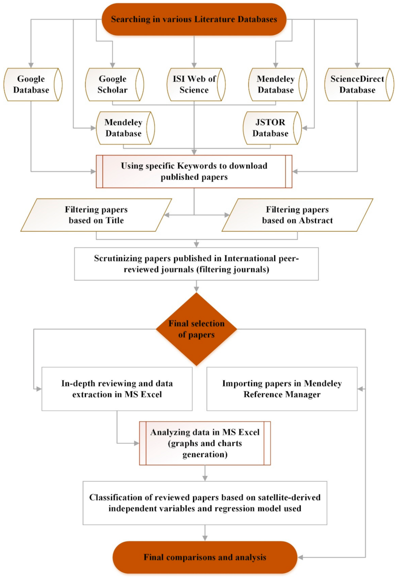
Along with these questions, the study also aimed to discuss and highlight the strengths and limitations of high-resolution optical satellite images in the context of global AGB dynamics.

2. Methodology

Figure 1 shows a detailed workflow of the literature review conducted. Based on specific keywords (see Table S2), the research papers were downloaded from well-known and famous literature databases, including Google Scholar, ISI Web of Science, Mendeley, ScienceDirect, Scopus, JSTOR, etc.
The downloaded papers were filtered after going through their titles, abstracts, and the journals in which they were published, as only peer-reviewed international journals were selected for the literature review. The papers that used optical high-resolution remotely sensed data, with or without combining them other remotely sensed datasets, that had a ≤5 m spatial resolution, were selected. After carefully selecting the final papers, the papers were classified based on (i) satellite-derived independent variables and (ii) the regression model used. An in-depth review followed, and the data were organized in Microsoft Excel software. Graphs and charts were generated that gave a clear overall picture of the frequency of the different regression models and satellite-derived independent variables used over time using high-resolution optical data. In order to achieve the objectives of the study, the extracted data (e.g., satellite-derived parameters, information about the sensor being used, the overall accuracy achieved, etc.) were further processed to compute sensor-wise estimated mean AGB and root mean square error (RMSE). Each study was analyzed and the overall accuracies of the estimated AGB were discussed. These accuracies were reported in the context of the satellite-derived variables and regression models used in each study. RMSE and AGB estimation accuracies helped us to identify the overall best performance of different sensors.

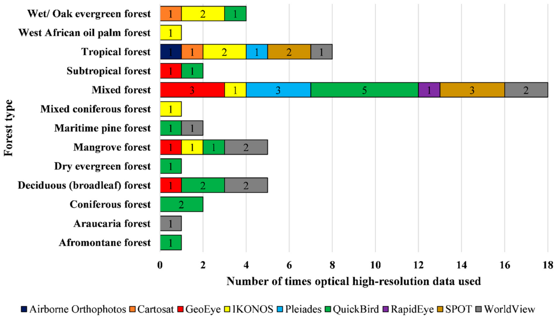
3. Geographical Areas

According to 44 peer-reviewed articles published in the 15 years (2004–2019), twenty-one studies were conducted in Asia, eight in North America and Africa, five in South America, and four in Europe (Figure S1). Among all the high-resolution optical satellites, QuickBird, WorldView, and IKONOS were mostly used for estimation and mapping forest biomass (Table 1).

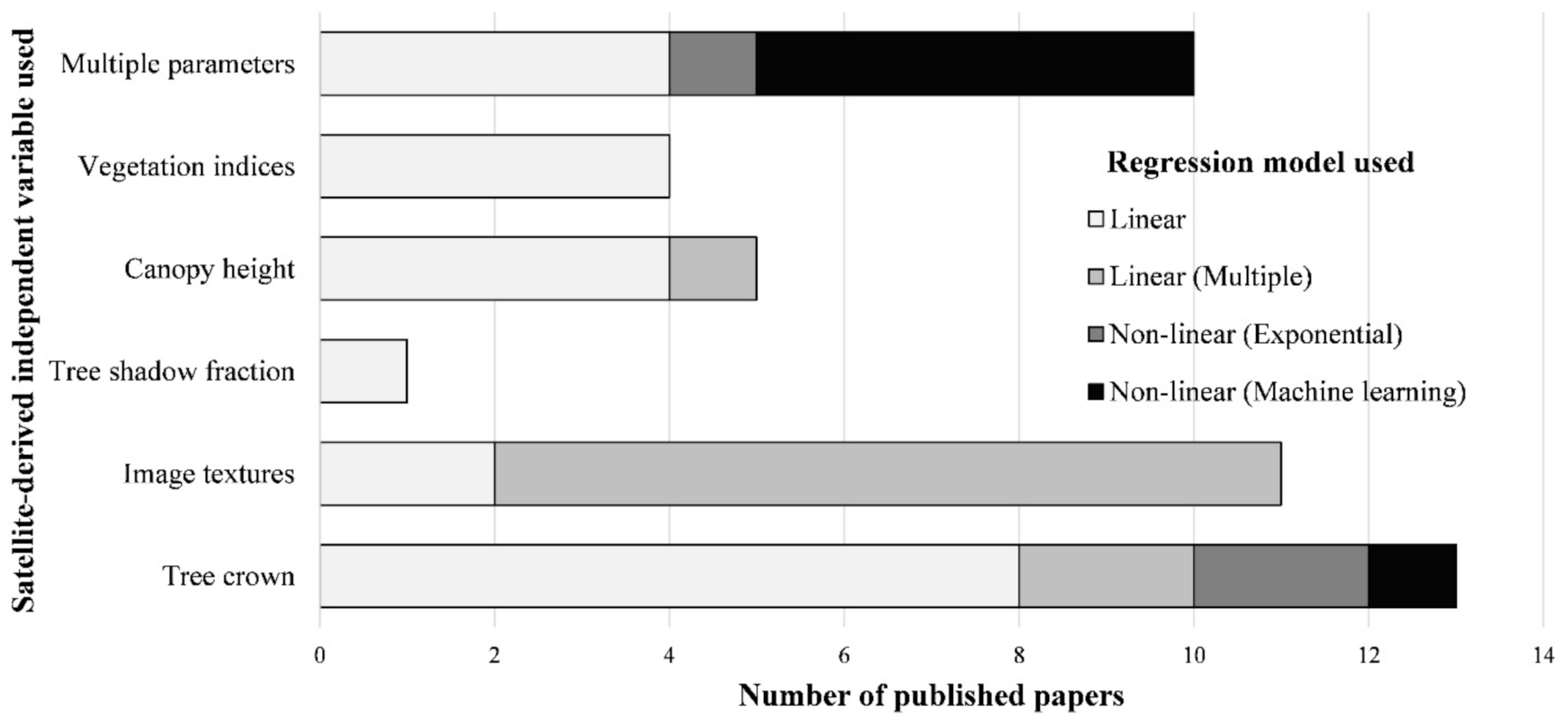
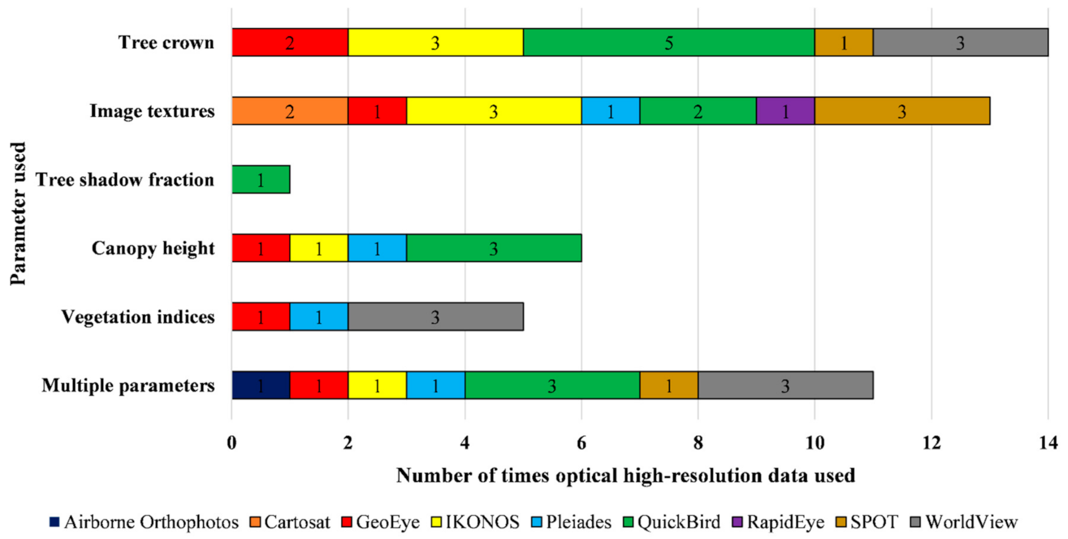
4. Satellite-Derived Independent Variables and Regression Techniques Used for AGB Modeling

Different satellite-derived independent variables were used to quantify and map AGB. According to the literature review, thirteen studies utilized tree crowns, eleven used image textures, five utilized canopy height, four utilized vegetation indices, ten utilized multiple variables, and only one utilized tree shadow fraction as the satellite-derived independent variable for the prediction of AGB using different regression models, including linear, linear (multiple), non-linear (exponential), and non-linear (machine learning) (Figure 2).

4.1. Tree Crown

Tree crown is a vital variable in developing allometric equations for AGB estimations and, in some cases, can explain more variations in estimating AGB than tree height [8]. Satellite-derived tree crown data can significantly affect AGB estimations using different regression models and the overall performance of those regression models [9]. The following studies used satellite-derived tree crown as a fundamental independent variable to map AGB using various regression models:

4.1.1. Linear Regression Models

The study by Clark et al. [10] in the tropical rain forest of Costa Rica using IKONOS satellite data with a linear regression model was based on basal area (BA) and AGB from the stem. They correlated the crown area measurement from the ground, and the crown area measured in the image, determining the tree’s size, location, mortality, and growth.
Likewise, Soenen et al. [11] conducted a study using a geometric optical canopy reflectance (CR) model in multiple forward mode (MFM) using SPOT-5 imagery in the mountainous terrain of the conifer and deciduous forests of Canada. The estimated tree crown dimensions and stem density for satellite image pixels were linked with plot-level AGB through linear modeling.
Moreover, Hirata et al. [12] conducted a study on the estimation of AGB in the mangrove forests in Thailand, wherein they examined the linear allometric relationship between the tree crown area derived from the QuickBird panchromatic data along with the multispectral data using the watershed method, an object-based image analysis (OBIA) technique, and stem diameter measured in the field for individual trees.
Additionally, Hussin et al. [7] evaluated an OBIA technique on GeoEye-1 high-resolution satellite images and 92 field sample plots for biomass estimation in Nepal’s hilly forests. The study used a linear regression model to develop a relationship between tree crown projection area (CPA) and field-based AGB values.
Similarly, Mbaabu et al. [13] conducted another study to compare two forest management regimes in Nepal’s Siwalik region. They used field data with fused GeoEye-1 satellite images and airborne LiDAR data in a linear regression model to estimate and map AGB. They developed the statistical relationship of LiDAR-derived canopy heights, GeoEye-1-derived CPA, and field-based AGB to map AGB for the entire study area.
Phua et al. [14] developed a linear regression model for tree density, based on field measured diameter at breast height (DBH) versus tree crown area delineated from IKONOS images. According to this study, the DBH allometric model explained that 74% of the data variance and extracted tree crown area strongly correlated with the field-measured DBH.
The study by Gonçalves et al. [15] studied allometric functions and temporally estimated AGB dynamics for Pinus pinaster using crown horizontal projection for a study area in Portugal. QuickBird (for the years 2004 and 2007) and WorldView-2 (for the year 2011) images were classified using OBIA to extract crown horizontal projections of pine stands and correlated these with field-based AGB. Out of six fitted models (four for forest field data and two for satellite image data), the best one estimated AGB as 32.3 tons h−1 in 2004, 16.3 tons h−1 in 2007, and 10.8 tons h−1 in 2011.
Phua et al. [16] assessed AGB using high-resolution optical imagery in an intact and degraded tropical rainforest in Malaysia. A simple linear regression model was generated as among the field-derived variables and satellite-based variables, DBH and crown dimensions correlated significantly (r = 0.87). Fifty square plots with trees of DBH > 10 cm were surveyed and, using IKONOS imagery, 1584 upper-canopy tree crowns were extracted from these plots to generate the model. The study concluded with a discussion on using published allometric equations to monitor and estimate AGB in intact and degraded tropical forests in the context of the UN-REDD+ program.

4.1.2. Linear (Multiple) Regression Models

Karna et al. [17] conducted a study to quantify and map carbon stocks at a tree species level using WorldView-2 satellite images, field data, and airborne LiDAR data using multiple linear models in the tropical forests of Nepal. The multiple linear regression was generated between the response variables (field-based carbon stock) and the explanatory variables (CPA and LiDAR-derived height).
The study in this regard by Mohd Zaki et al. [18] aimed to construct allometric equations for live AGB in Malaysia’s Selangor district. WorldView-3 imagery and LiDAR data were used to calculate the independent variables of tree height and tree crowns used in AGB calculations to be correlated with field-based variables of tree height, CPA, DBH, and AGB. Out of several of the best data-fitted multiple regression models, six were selected for further examination. Based on further investigations, field-only, field and satellite-based, and satellite-based-only models were discussed, in which predicted AGB ranged across about 0.72–13.56 tons tree−1 using the former model, 0.69–14.00 tons tree−1 using the middle model, and 0.77–16.31 tons tree−1 using the later model.

4.1.3. Non-Linear (Multiple and Exponential) Regression Models

Moreover, Hirata et al. [19] investigated the non-linear (exponential) relationship between DBH-based allometric models and crown area extracted from QuickBird panchromatic data for two tree species: (1) Cryptomeria japonica and (2) Chamaecyparis obtusa in the Nakatsugawa and Yoshikawa watersheds in the Shimanto River basin of Japan’s Shikoku Region.
Likewise, Gonzalez et al. [20] calculated forest carbon densities and uncertainties from QuickBird, LiDAR, and field measurements in California using a non-linear (exponential) model. This non-linear (exponential) model was developed from field-based aboveground live tree carbon density and LiDAR-derived heights and QuickBird-derived tree crown diameters.

4.1.4. Non-Linear (Machine Learning) Regression Models

Mora et al. [21] demonstrated a regression tree approach for modeling the average stand height and biomass of Canada’s mixed forests from QuickBird panchromatic imagery using the OBIA approach to develop homogenous segments for individual tree crowns. They used a regression tree to predict mean stand height from stand-level metrics (extracted from the images’ gray levels and within-stand objects relating to individual tree crown characteristics).

4.2. Image Textures

In recent years, scientists are leaning more towards using texture-based modeling of AGB estimation, as it provides more possibilities in various contexts [22]. The texture is an essential variable for estimating AGB, as it shows the high variance in tree crowns when using high-resolution satellite data [23]. The following studies used image texture as the primary/sole independent variable for estimating and mapping AGB using different regression models:

4.2.1. Linear Regression Models

Ouma and Tateishi [24] carried out a study in a mixed vegetation area of central Kenya, using QuickBird and Landsat Enhanced Thematic Mapper Plus (ETM+) satellite data and a linear model by optimization of second-order gray-level texture for estimating AGB. The study results illustrated that the integration of near infrared (NIR) spectral band entropy and second-moment texture measurements provided much better results. The study also concluded that in AGB estimation, the size (height), age, species, inherent spatial structure (natural or planted), and crown size of the vegetation tree species and texture types play an essential role in the estimation and mapping of AGB.
The study by Gascón et al. [23] estimated national-level AGB over Tanzania. They used generalized linear, non-linear exponential, and non-linear machine learning (random forest and support vector machine) methods to develop regressions among the input variables and AGB using RapidEye optical remote sensing satellite imagery. They extracted many textural and reflectance measurements, including simple ratios, band means, various vegetation indices, and other textural information to develop correlations among the field-based AGB measurements from plots and these variables. On the national level, they calculated a mean of 22.1 tons ha−1 AGB.

4.2.2. Linear (Multiple) Regression Models

Proisy et al. [25] performed a study in mangrove forests for AGB in French Guiana, Africa with linear (multiple regression) using IKONOS data through the Fourier-based textural ordination (FOTO) method, which computes the texture indices of tree canopy grain by performing a standardized principal component analysis (PCA). These textural indices were correlated with field-based biomass to predict AGB spatially in the entire study area.
Moreover, Nichol and Sarker [26] explored the potential of SPOT-5 and ALOS advanced visible and near infrared radiometer Type 2 (AVNIR-2) texture indices for quantification of biomass by developing multiple correlations with the biomass of 50 field plots. According to this study, they obtained significant improvements in biomass quantification while using the ratio of texture variables, among other texture indices.
Ploton et al. [27] assessed the AGB of the wet evergreen forests of the Western Ghats in India using Google Earth’s free IKONOS images in combination with the FOTO method, and field-observed stand structure parameters (including tree density, total BA, and AGB) using linear (multiple) relationships. The study results illustrated that the FOTO method provides better retrieval of AGB using Google Earth data, which can be replicable.
Bastin et al. [28] conducted a study in the Congo, Africa, wherein they acquired indices from two different sensors (GeoEye-1 and QuickBird) for calibrating a piecewise AGB inversion model from a sample collected from the heterogeneous forest area through the FOTO method. They developed multiple linear correlations between the main textural characteristics and AGB from field data. Their result showed a good agreement between predicted and observed AGB, which was confirmed by cross-validation.
Likewise, Singh et al. [29] conducted a study on the estimation of biomass of a mixed forest of a tropical oil palm forest in Sabah, Malaysian Borneo, using SPOT-5 with the FOTO method. They were able to retrieve high AGB values of various forest types correctly by developing multiple correlations with the field-based AGB values.
Ploton et al. [30] used Fourier and lacunarity canopy texture analysis for mapping the AGB of tropical forests using Pleiades images over four counties in three different continents. They introduced a new model developed using FOTO and lacunarity texture (FLE) indices to assess precision and accuracy in estimating forest AGB. They formed correlations among field-based variables (DBH, tree height, trunk height, and crown diameter) and satellite-derived variables (gap fraction, tree height, DBH, crown diameter, basal area, etc.) to map AGB across all the tropical forests under study.
The FOTO technique was used by Reddy et al. [31] for addressing the issue of saturation in high biomass ranges for predicting AGB in a wet evergreen forest in India. The study also discussed the impact of spatial resolutions in predicting AGB at large landscape scales using Cartosat-1 and IKONOS satellite imagery. In the context of satellite view geometry, the study showed the better performance of Cartosat-1 imageries (2.5 m), with a computed RMSE of 18%, compared with IKONOS (1 m), with 15% RMSE, in resolving texture information using the FOTO technique to predict AGB. They developed a multivariate correlation among field- and satellite-derived AGB for mapping AGB.
A similar study by Pargal et al. [32] addressed the saturation of remote sensing signals using Cartosat-1 imagery data in dry deciduous to evergreen forests in the Western Ghats of India. NDVI was used to calibrate texture–AGB models, which used complementary information to texture information while predicting AGB by correlating it to field-based measurements, including DBH, tree height, and AGB. A consistent texture–AGB relationship (R2 = 0.76) was obtained in this study compared with other tropical forests of the world using a solid FOTO technique, estimating AGB as exceeding 500 tons ha−1 in the study area.
Textural combination techniques were used by Hlatshwayo et al. [33] to estimate FAGB in a tropical, dry, reforested site located in South Africa, using pan-sharpened SPOT-6 imagery. They used random forests to estimate AGB using raw band textures, two-band textures, and three-band texture techniques by developing multiple correlations with field-observed AGB. For model formation, they used 63 out of 90 35 × 35 m field plots and were able to quantify 2962.90 tons ha−1 of mean AGB. This mean was extracted for two plantation periods between 2009–2011 and 2011–2013 in the study area.

4.3. Tree Shadow Fraction

Tree shadow fraction is another critical satellite-derived variable correlated with several forest structural characteristics [34]. In this review, we found only one study that primarily used the tree shadow approach to map AGB using linear regression model as follows:

Linear Regression Models

Leboeuf et al. [34] proposed a method over the northern boreal forest of eastern Canada for estimation and mapping the AGB of black spruce (Picea mariana) using 108 ground sample plots and QuickBird satellite data. They developed a linear regression between ground-based biomass values versus extracted tree shadow fraction (SF) as a predictive variable from the QuickBird images.

4.4. Canopy Height

Canopy height is a critical variable used to map AGB, as it directly correlates with biomass quantification and is a crucial satellite-derived variable for estimating AGB in dense forest structures [22]. Satellite-based canopy height calculation has aided several studies for precise AGB mapping as described below:

4.4.1. Linear Regression Models

St-Onge et al. [35] demonstrated the use of a combination of stereo IKONOS images and a LiDAR digital terrain model (DTM) to measure and map tree canopy height and biomass. For this, they generated a canopy height model (CHM), and plot-wise dominant height was extracted using this IKONOS-LiDAR CHM after validation by field data. The field data on AGB was linearly correlated with the CHM and used to generate an AGB map of the study area.
Moreover, Sousa et al. [36] developed a methodology to estimate AGB for Quercus rotundifolia in the evergreen oak forest in Portugal, using QuickBird satellite imagery. They adopted multi-resolution satellite imagery segmentation and an object-oriented classification method to calculate the area of the tree canopy’s horizontal projection from field-based AGB values in a linear regression model.
Koju et al. [37] used a linear regression model to develop a relationship between tree canopy cover (TCC) and forest aboveground biomass (FAGB) to extrapolate AGB using GeoEye-1 imagery along with Landsat-8 and Google Earth’s very high-resolution imagery. The extrapolation resulted in an estimated AGB over the entire study area (a subtropical forest in a watershed of Nepal). Before applying the extrapolation, they also used multivariate adaptive regression splines (MARS), a machine learning regression, to model the relationship between the forest AGB of Google Earth’s high-resolution imagery (virtual plots) and the predictive parameters of Landsat derivatives (bands, normalized difference vegetation index (NDVI), etc.). Out of 50 plots, 30 plots were utilized for model formation, while the remaining 20 were used for model validation. They calculated an average forest aboveground carbon (FAGC) of 260 tons ha−1 compared with a field-based average of 249 tons ha−1.
The latest study in this regard by Hosseini et al. [38] estimated dry and fresh AGB in a semi-arid region of Iran encompassing mixed forest types. Using CHM derived from Pleiades-1B stereo imagery, they linearly regressed field measurements using DBH, crown diameter, and stem length to map AGB in the entire study area. Their study proved that using stereo imagery pairs can effectively estimate AGB in semi-arid plantations around pollutant industrial areas for continuous monitoring.

4.4.2. Linear (Multiple) Regression Models

Hyde et al. [39] conducted a study for wildlife habitat analysis in a mixed coniferous forest using a multi-sensor (QuickBird, LiDAR, Landsat ETM+, and Synthetic Aperture Radar (SAR)/Interferometric Synthetic Aperture Radar (InSAR)) with linear (multiple regression) models in Northern America. The study concluded that for estimating tree canopy height and AGB, LiDAR data provided the best results as a single sensor and integrated with ETM+ metrics to evaluate the large tree structure. According to the findings of the study, QuickBird and SAR/InSAR are essentially redundant.

4.5. Vegetation Indices

By their ability to map vegetation density, vegetation indices produce strong correlations with AGB [40]. Several vegetation indices, sensitive to fluctuations in biomass, are available today, and comparative studies are being conducted in this regard to choose the best vegetation index for biomass mapping [41,42]. Out of all the models, researchers have only used linear and non-linear (machine learning) regression models for mapping AGB. The following are the details of the studies that used different vegetation indices to map AGB:

4.5.1. Linear Regression Models

Clerici et al. [43] developed an AGB estimation and mapping method for the secondary Andean forests near Bogotá, Colombia. They used six different vegetation indices derived from GeoEye-1 and Pleiades-1A satellite imagery and produced a linear correlation with field-measured AGB. According to their findings, the ratio vegetation index (RVI) had the most satisfactory AGB mapping results among all the indices.
The second study by Basso et al. [44] estimated the AGB of Araucaria angustifolia trees using vegetation indices extracted from WorldView-2 imagery. Vegetation indices including simple reason (SR), NDVI, and soil adjusted vegetation index (SAVI) were used, whereas NDVI showed the most promising results and correlation with AGB.

4.5.2. Non-Linear (Machine Learning) Regression Models

Mutanga et al. [45] explored the possibility of estimating biomass in densely vegetated mangroves in South Africa using NDVI (developed from all possible two-band combinations) computed from WorldView-2 and field-based fresh AGB through the random forest model.
Zhu et al. [46] used a backpropagation artificial neural network (BP ANN) for calculating six vegetation indices: NDVI, simple ratio index (SRI), difference vegetation index (DVI), etc. These vegetation indices used field-based AGB to model and map AGB in the entire study area.

4.6. Multiple Variables

Many reviewed studies used different independent variables for improving AGB mapping, including satellite-derived spectral bands, vegetation indices, textural indicators, etc. The details of these studies are as follows:

4.6.1. Linear (Multiple) Regression Models

A study was carried out by Fuchs et al. [47] on estimating and mapping aboveground carbon (AGC) stocks in the deciduous forest of the Siberian tundra by combining QuickBird, ASTER satellite data, and field inventory data with a multiple linear regression (MLR) model and the non-parametric K nearest neighbors (K-NN) classifier. They used Pearson’s correlation between field-observed AGC and satellite-derived variables, including the original satellite bands, vegetation indices, and texture metrics. Their results showed high spatial variability with carbon, reflecting the highly heterogamous conditions.
Castillo-Santiago et al. [48] explored a methodology of estimating the BA, tree volume, and biomass of the Lacandon rainforest in the Marqués de Comillas region in Chiapas, Mexico. SPOT-5 multispectral satellite images with 87 ground plots were used to provide sufficient information to develop a satisfactory regression model to predict tree canopy height, bole volume, and AGB. They also used Pearson correlations among 14 satellite-derived variables (including spectral bands, principal components, vegetation indices, and texture measures) and four field plot variables (BA, canopy height, bole volume, and AGB) to map AGB spatially over the entire study area.
Hirata et al. [49] performed tropical FAGB estimation using QuickBird satellite imagery and selective LiDAR measurements in a study area in Cambodia. They used multiple regression analysis in a two-step method in which first they correlated the AGB from LiDAR to field-based AGB values; secondly, they linked this model, as a dependent variable, to reflectance values from each band of the QuickBird satellite imagery.
The latest study in this regard by Reyes-Palomeque et al. [50] combined LiDAR data and Airborne Orthophotos (Vexcel UltraCam LP digital camera) to estimate AGB in tropical dry forests in Mexico. They estimated AGB in two different tropical dry forests, including semi-deciduous and semi-evergreen forests, using three multiple regression models. They used field-based variables, including DBH, height, and wood density, with the satellite-derived variables of tree height, forest canopy, vegetation indices, and spectral bands to develop MLR models. They used the results from LiDAR, airborne orthophotos and a combination of both. They concluded that both provided accurate results for AGB estimation, but this differed with forest type and its structural complexity. However, combining both datasets provided the best estimation for AGB in complex forest environments.

4.6.2. Non-Linear (Multiple and Exponential) Regression Models

Thenkabail et al. [51] conducted a study to estimate biomass and carbon stocks in the oil palm plantations of African-derived savannahs using IKONOS data and several models (including linear, multi-linear, and non-linear/exponential). The non-linear (exponential) model proved to be the best developed among the field-based dry biomass and IKONOS-based bands and indices (NDVI). They emphasized, through the results, the lack of additional spectral bands in the IKONOS sensor.

4.6.3. Non-Linear (Machine Learning) Regression Models

Similarly, Chen et al. [52] demonstrated the use of an OBIA framework through the support vector regression modeling technique to predict AGB from LiDAR transects, QuickBird imagery in Quebec, Canada. They used LiDAR data to estimate canopy height, QuickBird imagery to extract variables (mean spectral bands, image texture, and shadow fraction), and field measurements (canopy height, AGB, and volume) for modeling AGB in the entire study area using machine learning techniques).
Jachowski et al. [53] conducted a study to assess tree biomass and species diversity within the mangrove ecosystem on the Andaman Coast of Thailand using GeoEye-1 (variables including spectral bands, band ratios, and NDVI) combined with ASTER (for elevation) digital elevation models (DEM) and field-based tree biomass values. They found that support vector machines gave the best results among other Waikato Environment for Knowledge Analysis (WEKA) machine-learning algorithms.
Kattenborn et al. [54] applied the Random Forest model, generalized additive models (GAM), and two boosted algorithms: the generalized boosted regression model and the amplified version of the GAM. These machine learning techniques were used to model AGB in the entire study area using the spectral bands of remotely sensed data, principal components, vegetation indices, satellite-derived CHM, and field-based AGB.
Maack et al. [55] used spectral, textural, and photogrammetric information from stereo satellite data (Pleiades and WorldView-2) combined with field-based AGB to estimate forest biomass across two test sites located in Chile and Germany. They compared the Random Forest model performances of different predictor sets (spectral, textural, and photogrammetric), forest inventory designs, and filter sizes (texture information).
Machine learning regression algorithms (Random Forest and support vector machine) were applied by Dhanda et al. [56] for biomass estimation in tropical moist deciduous forests in India. They used spaceborne LiDAR (ICESat/Geoscience Laser Altimeter System (GLAS)) data along with WorldView-2 imagery to derive biomass estimation parameters from 40 (20 m) circular plots. The six most important variables (tree height, textures, spectral bands, etc.) derived from LiDAR and WorldView-2 satellite imagery combined with field-based height and biomass observations were utilized to model AGB using machine learning techniques. For comparison, they also used MLR for biomass estimation.
Among all the satellite-derived variables, the tree crown was the most used variable in all reviewed articles in this study (Figure 3). QuickBird was used in most of the studies (14) to extract this variable, while SPOT was used only once. It can also be observed that QuickBird satellite data were used to extract almost all the satellite-derived independent variables except vegetation indices, which were the least used after the tree shadow fraction variable. After tree crown, the most widely used variable was image textures, followed by multiple variables, canopy height, vegetation indices, and tree shadow fraction. Similarly, after QuickBird, the researchers used GeoEye satellite data to extract diverse satellite-based independent variables (five) but these were not used by most studies (only six). The second most used satellite data were from WorldView, which was used to extract three different satellite-derived variables for AGB estimation. It can be inferred that QuickBird is widely used (i.e., the number of studies) and has the most diversely used satellite data among all other sensors.
For estimating AGB, most of the published studies (18) were performed on mixed forest (coniferous and deciduous) types, followed by tropical forests (eight), mangrove forests (five), and deciduous forests (five), and fewer were performed on other types of forests (Figure 4). It can be noted that QuickBird satellite data were used in the most diverse types of forests (nine forest types), followed by WorldView (six forest types) and IKONOS (five forest types); the remaining satellite sensors were used in less than five distinctive forest types. Because only a few published studies used optical high-resolution satellite images to quantify AGB, it is difficult to infer that one specific satellite sensor is best for all forest types; instead, looking at the accuracy they produce could be more interesting.

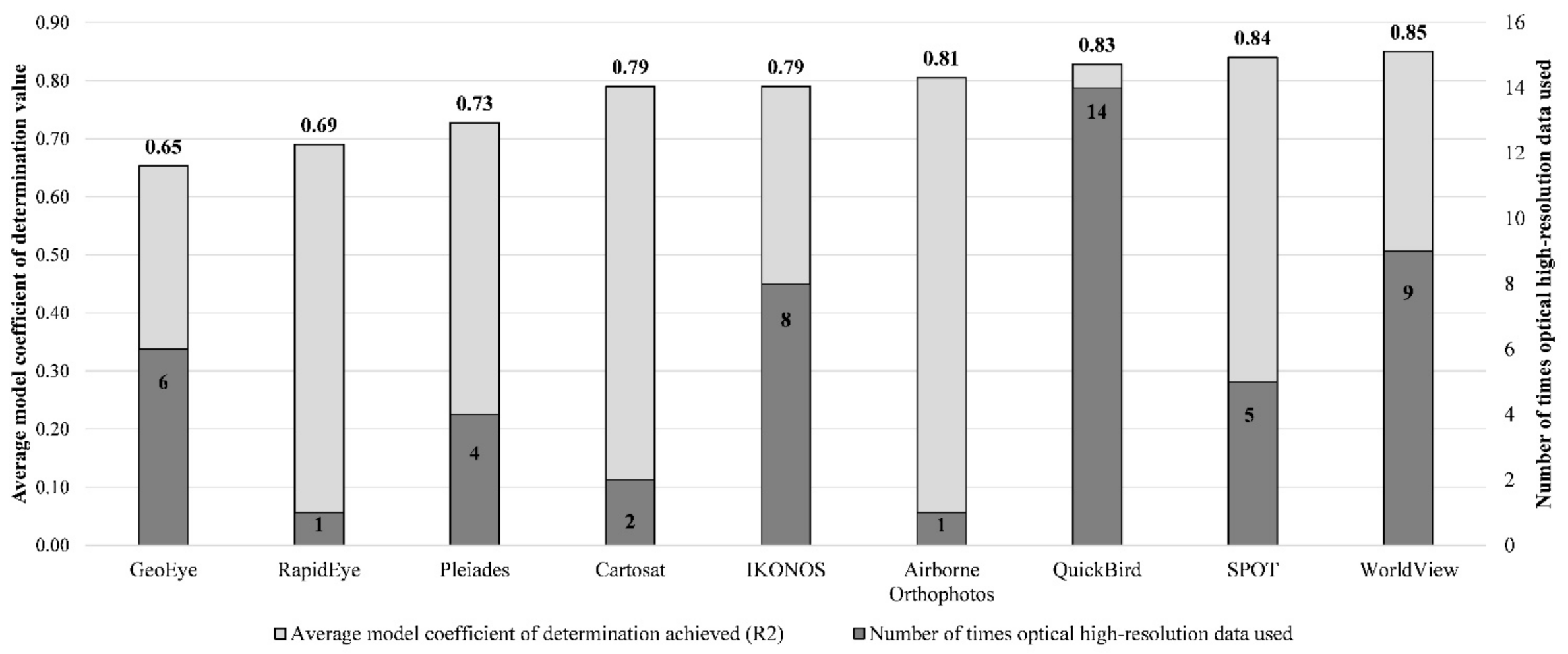
5. AGB Estimations and Reporting

Not all studies reported every parameter, including the biomass equation, the total number of samples for model formation, model accuracy, estimated mean AGB, etc., observed in this review.
A comparison of the cumulative estimated AGB (ton ha−1) against each sensor, as reviewed in this study, was carried out (Figure 5), and it showed that RapidEye exhibited the most negligible median value of 21.5 tons ha−1, while Pleiades presented a maximum median value of 359 tons ha−1.
Satellite imagery of IKONOS, QuickBird, and WorldView-2 was used to estimate AGB for at least four different continents in the world (Table S3). Other than these, Pleiades and SPOT-5 satellite data ranked second in spatial diversity to estimate AGB. It is noteworthy that no study was found in Australia and Oceania that used high-resolution (≤5 m spatial resolution) data for AGB estimation. As mentioned in Table 1, most of the studies took place in Asia and Africa (mostly in developing countries) compared with other continents. As developing countries are more concerned about the performance-based payment mechanisms under the REDD+ project, they tend to use the technologies and techniques transferred from the developed countries. This could be the reason why no or few studies were found in Australia and Oceania and other developed continents, as these developed regions tend to develop and use data fusion and integration techniques.

6. Accuracy Assessment of AGB Estimations

The coefficient of determination (R2) is universally used to determine and measure the variation in the dependent variable caused by the predictors used in different models [57]. Its value ranges from 0 to 1, with a higher value indicating more valid model results. This was the primary indicator reviewed for all the published studies and is described as follows:
Thenkabail et al. [51] obtained an overall accuracy of 88%–92% at the landscape level with 29.5 and 29.88 tons ha−1 of dry biomass of different age trees. Combining multi-sensors (LiDAR, Landsat ETM+, and SAR/InSAR) in the mixed coniferous forests produced a more accurate result (R2 = 0.83, RMSE = 66.6 tons ha−1) in comparison with the individual sensors used in the study by Hyde et al. [39]. Similarly, Ouma and Tateishi [24] carried out a study in Kenya with QuickBird and Landsat ETM+ satellite data and a linear model. They obtained 72% and 67.34% accuracy with the NIR and variance–texture bands, where the mean textures provided the best results in combination with NIR, presenting similar results (R2 = 0.684). In the study, contrast texture contributed good results (R2 = 0.753) as an independent variable for older pine trees, while for young pine trees, correlation texture offered good overall results (R2 = 0.741). Leboeuf et al. [34] estimated the biomass of 0.008 tons for young pine trees (3.5 years old) and 0.01 ton for older pine trees (6 years old). Models of stand height, volume, and biomass from Canada in combination with high-resolution images and in combination with LiDAR data were found to correlate with stand height (RMSE = 1.9 m), volume (RMSE = 9.9 m3 ha−1), and biomass (RMSE = 22.8 tons ha−1). Another study in North America’s California by Gonzalez et al. [20] compared and validated delineated tree crown diameters from QuickBird imagery against field measurements, with a significant correlation (R2 = 0.82). The study compared field-derived Lorey’s mean height with the stand-level LiDAR height metric and found a significant correlation for two study areas (Garcia–Mailliard: R2 = 0.94 and North Yuba: R2 = 0.89).
Furthermore, in Canada’s boreal forest, statistically, the QuickBird panchromatic imagery provided the best model results (R2 = 0.53 and RMSE = 2.84 m), with 84.6% falling within the acceptable error [34]. Moreover, Proisy et al. [25] studied how to develop FOTO indices from IKONOS imagery (2001 and 2003), with a good relationship between observed and predicted AGB (residual standard error-RSE¼ = 15%; R2¼ = 0.85) across a wide range of AGB levels from 26 tons ha−1 to 460 tons ha−1. AGB estimation with IKONOS by tree crown delineation in Borneo’s tropical forest showed 64% overall segmentation accuracy than the field observations, seeing a strong correlation between crown detection percent tree density. Meanwhile, the satellite-based crown area had the highest correlation with the field measured DBH. The DBH allometric model explained 74% of the data variance. Hussin et al. [7] conducted a study in the Ludhi Khola watershed, Gorkha district, Nepal, which assessed the accuracy of the region’s growth to be higher than that in the valley, following segmentation of 166 manually delineated reference tree crowns, and exhibited a segmentation accuracy of 68% and 58% gradually and overall, and 74% user and producer accuracy, with a 0.48 kappa statistic. Clerici et al. [43] attained model goodness of fit (R2 = 0.58, RMSE = 34.5 tons ha−1) for the best linear regression model through RVI (Table S2). The study of Ploton et al. [30] assessed the accuracy of Pleiades satellite images, with a significant relationship (R2 = 0.47) and reasonable error levels (<25% rRMSE) over 49 field plots with AGB 359 ± 98 tons ha−1. Phua et al. [16] used 25 plots for AGB validation and reached an accuracy of R2 = 0.812 and R2 = 0.7142 for intact and degraded forests, respectively. On the other hand, Pargal et al. [32] showed an accuracy of R2 = 0.76 with rRMSE = 17.1% while predicting AGB in the evergreen forests of the Western Ghats in India. Mohd Zaki et al. [18] showed a good accuracy of R2 = 0.914 for the best model among all other models used while predicting AGB in tropical lowland Dipterocarp forests in Malaysia. The study conducted by Dhanda et al. [56] explained 78.7% of the observed AGB. The study found that support vector machines (explained 88.7% of AGB) worked better when correlations among the subset of underlying variables and predicted variables existed. While, on the other hand, the Random Forests (explained 83.5% of AGB) regression algorithm worked better even if there was no correlation among the subset of underlying variables and predicted variables. Koju et al. [37] achieved a modeling-based coefficient of determination (R2) of 0.76, while this was 0.83 for the model validation. They used 30 (500 m2 circular) plots for model formation and 20 plots for model validation. Hirata et al. [49] established 57 field-based sample plots of either 30 m2 or 50 m2 to calculate AGB from the field to be used in the models. They found an overall accuracy of R2 of 0.90 (with an RMSE of 38.7 tons ha−1) and 0.73 (with an RMSE of 42.8 tons ha−1) for LiDAR measurements and QuickBird satellite imagery. Hlatshwayo et al. [33] used 27 (35 × 35 m) plots, out of 90, for model validation. Among all the textural band combination techniques, the three-band texture was able to yield the maximum overall predicted accuracy of R2 = 0.88. Random Forest regression outclassed multiple linear regression techniques in predicted accuracy (R2), ranging from 0.53 to 0.93 compared with 0.29 to 0.85. Reyes-Palomeque et al. [50] used 20 0.1 ha plots in the semi-deciduous forest and 28 plots in the semi-evergreen forest for AGB estimation in their study area. LiDAR and airborne orthophotos showed a regression (R2) fit of 0.82 and 0.70 in the semi-evergreen forest, and 0.88 and 0.91 in the semi-deciduous forest, respectively. Cross-validation results showed the accuracy (R2) of LiDAR and airborne orthophotos to be 0.62 (with RMSE = 35.5 tons ha−1) and 0.52 (with RMSE = 42.6 tons ha−1) in the semi-evergreen forest, and 0.85 (with RMSE = 14.4 tons ha−1) and 0.86 (with RMSE = 13.6 tons ha−1) in the semi-deciduous forest, respectively. Combining both datasets showed a better regression fit (R2) of 0.85 in a more complex forest structure with a validation accuracy (R2) of about 0.69 (with RMSE = 33.0 tons ha−1). Gascón et al. [23] used, after cleaning, readily available data from 500 plots to assess national level AGB in Tanzania. Using generalized linear regression, generalized exponential regression, Random Forest and support vector machine methods, they obtained accuracies of 0.39 (with RMSE = 41.81 tons ha−1), 0.32 (with RMSE = 44.55 tons ha−1), 0.69 (with RMSE = 30.00 tons ha−1), and 0.42 (with RMSE = 39.08 tons ha−1) respectively. All four methods produced a gain in the performance of the training dataset, with Random Forest having the best accuracy (R2 = 0.93, with RMSE = 15 tons ha−1) and were biased (overestimating low AGB, underestimating high AGB). Twenty-nine Araucaria angustifolia trees were sampled by Basso et al. [44], and, among all the vegetation indices they used, NDVI yielded the best results, with a 0.87 coefficient of determination and 38.56% relative error. The newest study by Hosseini et al. [38] used 48 field plots to estimate AGB in the semi-arid study area in Iran. They calculated total biomass and dry biomass with an overall coefficient of determination (R2) for all plantation types of 0.90 (RMSE = 24.92 tons ha−1) and 0.91 (RMSE = 12.74 tons ha−1), respectively.
Among the reported studies, QuickBird satellite data were not only used most frequently but also provided a high average model coefficient of determination (R2 > 0.8) (Figure 6). The highest cumulative model coefficient of determination (R2 > 0.9) was found for WorldView satellite data, even though it was used in only one study. The average model coefficient of determination of R2 > 0.8 was also observed for airborne orthophotos, IKONOS, and SPOT, among which, the former two were only used in one study, while the latter was used in four studies. All other sensors reported a cumulative model of coefficient of determination of R2 < 0.8. It may be noted that the figure presents only a rough estimation of the satellite sensors’ accuracy, as, without an assessment of the mean confidence interval, it cannot provide grounds for a statistical evaluation of the satellite sensors’ accuracy differences. This is because the number of published papers is too low to estimate the mean confidence interval.
Many studies use error budgeting methods to estimate output uncertainty and quantify the relative uncertainties of the model inputs [58]. It is imperative to assess the strength of models, as accuracy is essential in evaluating global carbon budgets [59]. However, none of the reviewed published papers in this study talked about the error budgeting factor, making it very difficult to rank a specific sensor or model for AGB estimations in complex forest environments.

7. Limitations and Challenges

In most high-resolution satellite images, the lack of spectral variation, the topography of the study area, and the shadows due to canopy and topography cause trouble in creating accurate and precise spatial AGB estimation models [3,60]. The impacts on AGB models due to reflectance caused by environmental conditions and shadows can be minimized through including vegetation indices as variables in the models. Even in complex vegetation stands, vegetation indices help us to understand the dynamic values and predict better AGB numbers. Geometric and/or ortho-rectification (especially in mountain areas) of the satellite images are vital to overcoming the distortions related to the sensor (e.g., jitter, view angle effects), the satellite (e.g., attitude deviations from nominal), and the Earth (e.g., rotation, curvature, relief) [4]. Most of the time, analysts prefer to rely on freely available DEM data to integrate rational polynomial coefficient (RPC) files due to the high cost of high-resolution DEMs.
A per-pixel-level representation of AGB and carbon stock values are rather difficult due to co-registration errors between satellite-derived independent biophysical variables and field collected biomass values. At the per-pixel level, registration errors between spatial and ground-measured variables can give a misleading accuracy measure of the AGB estimation [3,6]. For the conversion of measured forest inventory data to biomass, locally developed tree species-specific allometric equations are essential, but very often, researchers rely on some generalized globally available equation [61].
In some parts of the world, the limited number of studies quantifying aboveground biomass restricts the researchers to using only globally available allometric equations instead of species-specific local allometric equations that can produce more accurate and precise estimations [62]. Similarly, the absence of well-distributed field data, the incapability of optical sensors to present a strong correlation with forest AGB after tree canopy closure, and selection of the satellite sensors to be used for AGB estimations are among the other challenges and limitations [63].

8. Applications of High-Resolution AGB Estimations and Maps

The UN-REDD+ is an international framework designed by the United Nations (UN) to reduce deforestation and forest degradation emissions, support forest conservation practices, and enhance forest carbon stocks. Recent developments in Earth observation and the availability of high-resolution satellite imagery have boosted countries’ capacity, especially developing countries, to improve forest biomass estimations and other forest measurements [64]. Köhl [65] reported that the measurement, reporting, and verification (MRV) system for REDD+ requires high-resolution satellite data to precisely and accurately measure forest degradation and carbon emissions. NASA’s GEDI, NASA’s Ice Cloud and land Elevation Satellite (ICESat-2), and the NASA-Indian Space Research Organization (ISRO) Synthetic Aperture Radar (NISAR) are three upcoming active remote sensing products for estimating various forest structures and AGB as well [66]. The results produced by these products can be improved and validated using high-resolution optical data that, in turn, can improve the performance-based payment mechanism of the REDD+ program.
The literature review revealed that AGB estimation and mapping through high-resolution satellite data are being used for site-specific studies or small areas to produce accurate and reliable results. In most cases, in linear regression modeling, analysts’ biases prune the data back and forth to obtain accurate results based on the available sample plots and independent biophysical variables from satellite images. Thus, automatic machine learning models can provide better results using multiple variables but work as a black box. Based on the literature review, we realized that few studies talked about monitoring or quantification of AGB changes using high-resolution optical satellite images. In the future, this dimension needs to be explored using the same resolution of satellite data and methodology over the same areas.

9. Alternatives to Optical High-Resolution Satellite Data for AGB Estimations

High-resolution optical satellite data have been used along with other active (a system that uses its own radiation to illuminate the object under observation) and passive (a system that uses the naturally occurring radiation’s reflection) remotely sensed datasets. These datasets comprise low to medium (e.g., MODIS, Landsat, etc.), medium to high (e.g., aerial photographs, Sentinel, etc.), and high to very high (e.g., SAR, LiDAR, etc.) resolutions. The studies have suggested that the data collected through passive systems are usually less sensitive to vegetation structures because of their ability to capture only the reflected energy from the uppermost part of the vegetation, while the active systems like SAR and LiDAR have the ability to penetrate the vegetation to map the structures in detail, consequently producing better AGB estimates [67]. The review by Zolkos et al. [67] concluded that the airborne LiDAR metrics were more accurate than radar or other optical data, while the AGB models developed by incorporating multi-sensor data were even more accurate in estimating the AGB. Similarly, the review by Barbosa et al. [68] indicated the same issue of using optical-only data for estimating the AGB and using active system data to overcome this problem. Using airborne imagery and LiDAR is still a challenge in developing countries, as there are no spaceborne LiDAR data providing global coverage [69].
Similarly, the utilization of remotely sensed data from unmanned aerial vehicles (UAVs) depends on the area coverage and the operational costs involved [70]. Security concerns, licensing issues for using UAVs, and the lack of particular skill sets for processing and piloting the UAV missions are some of the hindrances to using airborne imagery for AGB estimations. The other options include medium- to high-resolution satellite imagery of the Landsat series (Landsat TM, Landsat ETM+, Landsat OLI, and the upcoming Landsat OLI2 in fall 2021 with a 30 m spatial resolution) and Sentinel-2 (with 10 m spatial resolution), which are being used by the researchers to overcome the cost and data processing issues of estimating AGB. The high-resolution optical data, which require relatively less expertise to process, are vital for AGB estimations and can be used in fusion or combination with other remotely sensed datasets to produce highly accurate AGB estimates.

10. Conclusions

Among the different satellite-derived independent variables, the tree crown was the most widely used variable, found by synthesizing 44 peer-reviewed articles, followed by the image textures and multiple parameters. Similarly, the most widely and diversely used regression model was linear regression, producing acceptable accuracies across different forest types. Linear regression was also the only regression model used against each satellite-derived independent variable, including the tree crown, image textures, tree shadow fraction, canopy height, vegetation indices, and multiple parameters. Keeping in view the complex forest environments, it is challenging to declare one specific sensor as the best among others, unanimously. However, QuickBird imagery, followed by WorldView and IKONOS imagery, was the most diversely used optical data and produced high R2 values in various forest types worldwide.
The spatial estimation of AGB is critical for many environmental, ecological, and forest studies, including the REDD+. In order to produce AGB estimations on various spatial scales, alternative options to optical high-resolution are available, including MODIS, Landsat, and Sentinel. Along with these, integrating optical data with active sensor data (LiDAR, radar, etc.) can also produce more accurate AGB estimations. Finally, the error budgeting of the estimated AGB is still an essential factor to be discussed in future studies.

Supplementary Materials

The following are available online at https://www.mdpi.com/article/10.3390/f12070914/s1. Figure S1: A catalog of 44 peer-reviewed published studies between 2004 to 2019 on forest AGB estimation and mapping through optical high-resolution satellite imagery (≤5 m spatial resolution). Table S1: A catalog of 44 peer-reviewed published studies between 2004 to 2019 on forest AGB estimation and mapping through optical high-resolution satellite imagery (≤5 m spatial resolution). Table S2: A list of keywords/terms used in searching for the literature. Table S3: A database of the methodology, accuracy, and average AGB values published in 44 peer-reviewed articles (2004–2019) for forest AGB estimation and mapping using high-resolution satellite imagery.

Author Contributions

Conceptualization, A.A. and H.G.; methodology, A.A., H.G. and S.R.A.; software, A.A.; validation, H.G. and S.R.A.; formal analysis, A.A.; investigation, A.A. and H.G.; writing—original draft preparation, A.A.; writing—review and editing, H.G. and S.R.A.; visualization, A.A.; supervision, H.G. and S.R.A.; project administration, S.R.A. All authors have read and agreed to the published version of the manuscript.

Funding

This research received no external funding.

Data Availability Statement

Data is contained within the article or Supplementary Material.

Acknowledgments

We would like to express our thanks to the management of the Institute of Space Technology (IST), the College of Earth and Environmental Sciences (CEES), and the Department of Geography, University of the Punjab for their support.

Conflicts of Interest

The authors declare no conflict of interest.

References

  1. Bindschadler, R.; Vornberger, P. Changes in the West Antarctic Ice Sheet since 1963 from declassified satellite photography. Science 1998, 279, 689–692. [Google Scholar] [CrossRef] [PubMed]
  2. Le Toan, T.; Quegan, S.; Davidson, M.W.J.; Balzter, H.; Paillou, P.; Papathanassiou, K.; Plummer, S.; Rocca, F.; Saatch, S.; Shugart, H.; et al. The BIOMASS Mission: Mapping global forest biomass to better understand the terrestrial carbon cycle. Remote Sens. Environ. 2011, 115, 2850–2860. [Google Scholar] [CrossRef] [Green Version]
  3. Lu, D. The potential and challenge of remote sensing-based biomass estimation. Int. J. Remote Sens. 2006, 27, 1297–1328. [Google Scholar] [CrossRef]
  4. Dowman, I.J.; Jacobsen, K.; Konecny, G.; Sandau, R. High Resolution Optical Satellite Imagery; Whittles Publishing: Scotland, UK, 2012; ISBN 978-184995-046-6. [Google Scholar]
  5. Song, C.; Dickinson, M.B. Extracting forest canopy structure from spatial information of high resolution optical imagery: Tree crown size versus leaf area index. Int. J. Remote Sens. 2008, 29, 5605–5622. [Google Scholar] [CrossRef]
  6. Gibbs, H.K.; Brown, S.; Niles, J.O.; Foley, J.A. Monitoring and estimating tropical forest carbon stocks: Making REDD a reality. Environ. Res. Lett. 2007, 2, 4. [Google Scholar] [CrossRef]
  7. Hussin, Y.A.; Gilani, H.; Van Leeuwen, L.; Murthy, M.S.R.; Shah, R.; Baral, S.; Tsendbazar, N.E.; Shrestha, S.; Shah, S.K.; Qamer, F.M. Evaluation of object-based image analysis techniques on very high-resolution satellite image for biomass estimation in a watershed of hilly forest of Nepal. Appl. Geomatics 2014, 6, 59–68. [Google Scholar] [CrossRef]
  8. Goodman, R.C.; Phillips, O.L.; Baker, T.R. The importance of crown dimensions to improve tropical tree biomass estimates. Ecol. Appl. 2014, 24, 680–698. [Google Scholar] [CrossRef] [Green Version]
  9. Li, C.; Li, Y.; Li, M. Improving forest aboveground biomass (AGB) estimation by incorporating crown density and using Landsat 8 OLI images of a subtropical forest in western Hunan in central China. Forests 2019, 10, 104. [Google Scholar] [CrossRef] [Green Version]
  10. Clark, D.B.; Read, J.M.; Clark, M.L.; Cruz, A.M.; Dotti, M.F.; Clark, D.A. Application of 1-m and 4-m resolution satellite data to ecological studies of tropical rain forests. Ecol. Appl. 2004, 14, 61–74. [Google Scholar] [CrossRef]
  11. Soenen, S.A.; Peddle, D.R.; Hall, R.J.; Coburn, C.A.; Hall, F.G. Estimating aboveground forest biomass from canopy reflectance model inversion in mountainous terrain. Remote Sens. Environ. 2010, 114, 1325–1337. [Google Scholar] [CrossRef]
  12. Hirata, Y.; Tabuchi, R.; Patanaponpaiboon, P.; Poungparn, S.; Yoneda, R.; Fujioka, Y. Estimation of aboveground biomass in mangrove forests using high-resolution satellite data. J. For. Res. 2014, 19, 34–41. [Google Scholar] [CrossRef]
  13. Mbaabu, P.R.; Hussin, Y.A.; Weir, M.; Gilani, H. Quantification of carbon stock to understand two different forest management regimes in Kayar Khola watershed, Chitwan, Nepal. J. Indian Soc. Remote Sens. 2014, 42, 745–754. [Google Scholar] [CrossRef]
  14. Phua, M.-H.; Ling, Z.-Y.; Wong, W.; Korom, A.; Ahmad, B.; Besar, N.A.; Tsuyuki, S.; Ioki, K.; Hoshimoto, K.; Hirata, Y.; et al. Estimation of Above-Ground Biomass of a Tropical Forest in Northern Borneo Using High-resolution Satellite Image. J. For. Environ. Sci. 2014, 30, 233–242. [Google Scholar] [CrossRef] [Green Version]
  15. Gonçalves, A.C.; Sousa, A.M.O.; Mesquita, P.G. Estimation and dynamics of above ground biomass with very high resolution satellite images in Pinus pinaster stands. Biomass Bioenergy 2017, 106, 146–154. [Google Scholar] [CrossRef] [Green Version]
  16. Phua, M.H.; Ling, Z.Y.; Coomes, D.A.; Wong, W.; Korom, A.; Tsuyuki, S.; Ioki, K.; Hirata, Y.; Saito, H.; Takao, G. Seeing trees from space: Above-ground biomass estimates of intact and degraded montane rainforests from high-resolution optical imagery. IForest 2017, 10, 625–634. [Google Scholar] [CrossRef] [Green Version]
  17. Karna, Y.K.; Hussin, Y.A.; Gilani, H.; Bronsveld, M.C.; Murthy, M.S.R.; Qamer, F.M.; Karky, B.S.; Bhattarai, T.; Aigong, X.; Baniya, C.B. Integration of WorldView-2 and airborne LiDAR data for tree species level carbon stock mapping in Kayar Khola watershed, Nepal. Int. J. Appl. Earth Obs. Geoinf. 2015, 38, 280–291. [Google Scholar] [CrossRef]
  18. Mohd Zaki, N.A.; Latif, Z.A.; Suratman, M.N. Modelling above-ground live trees biomass and carbon stock estimation of tropical lowland Dipterocarp forest: Integration of field-based and remotely sensed estimates. Int. J. Remote Sens. 2018, 39, 2312–2340. [Google Scholar] [CrossRef]
  19. Hirata, Y.; Tsubota, Y.; Sakai, A. Allometric models of DBH and crown area derived from QuickBird panchromatic data in Cryptomeria japonica and Chamaecyparis obtusa stands. Int. J. Remote Sens. 2009, 30, 5071–5088. [Google Scholar] [CrossRef]
  20. Gonzalez, P.; Asner, G.P.; Battles, J.J.; Lefsky, M.A.; Waring, K.M.; Palace, M. Forest carbon densities and uncertainties from Lidar, QuickBird, and field measurements in California. Remote Sens. Environ. 2010, 114, 1561–1575. [Google Scholar] [CrossRef]
  21. Mora, B.; Wulder, M.A.; White, J.C. Segment-constrained regression tree estimation of forest stand height from very high spatial resolution panchromatic imagery over a boreal environment. Remote Sens. Environ. 2010, 114, 2474–2484. [Google Scholar] [CrossRef]
  22. Abbas, S.; Wong, M.S.; Wu, J.; Shahzad, N.; Irteza, S.M. Approaches of satellite remote sensing for the assessment of above-ground biomass across tropical forests: Pan-tropical to national scales. Remote Sens. 2020, 12, 3351. [Google Scholar] [CrossRef]
  23. Gascón, L.H.; Ceccherini, G.; Haro, F.J.G.; Avitabile, V.; Eva, H. The potential of high resolution (5 m) RapidEye optical data to estimate above ground biomass at the national level over Tanzania. Forests 2019, 10, 107. [Google Scholar] [CrossRef] [Green Version]
  24. Ouma, Y.O.; Tateishi, R. Optimization of Second-Order Grey-Level Texture in High-Resolution Imagery for Statistical Estimation of Above-Ground Biomass. J. Environ. Inform. 2006, 8, 70–85. [Google Scholar] [CrossRef]
  25. Proisy, C.; Couteron, P.; Fromard, F. Predicting and mapping mangrove biomass from canopy grain analysis using Fourier-based textural ordination of IKONOS images. Remote Sens. Environ. 2007, 109, 379–392. [Google Scholar] [CrossRef]
  26. Nichol, J.E.; Sarker, M.L.R. Improved biomass estimation using the texture parameters of two high-resolution optical sensors. IEEE Trans. Geosci. Remote Sens. 2011, 49, 930–948. [Google Scholar] [CrossRef] [Green Version]
  27. Ploton, P.; Pélissier, R.; Proisy, C.; Flavenot, T.; Barbier, N.; Rai, S.N.; Couteron, P. Assessing aboveground tropical forest biomass using Google Earth canopy images. Ecol. Appl. 2012, 22, 993–1003. [Google Scholar] [CrossRef] [Green Version]
  28. Bastin, J.F.; Barbier, N.; Couteron, P.; Adams, B.; Shapiro, A.; Bogaert, J.; De Cannière, C. Aboveground biomass mapping of African forest mosaics using canopy texture analysis: Toward a regional approach. Ecol. Appl. 2014, 24, 1984–2001. [Google Scholar] [CrossRef]
  29. Singh, M.; Malhi, Y.; Bhagwat, S. Biomass estimation of mixed forest landscape using a Fourier transform texture-based approach on very-high-resolution optical satellite imagery. Int. J. Remote Sens. 2014, 35, 3331–3349. [Google Scholar] [CrossRef]
  30. Ploton, P.; Barbier, N.; Couteron, P.; Antin, C.M.; Ayyappan, N.; Balachandran, N.; Barathan, N.; Bastin, J.F.; Chuyong, G.; Dauby, G.; et al. Toward a general tropical forest biomass prediction model from very high resolution optical satellite images. Remote Sens. Environ. 2017, 200, 140–153. [Google Scholar] [CrossRef]
  31. Reddy, S.S.; Rajashekar, G.; Jha, C.S.; Dadhwal, V.K.; Pelissier, R.; Couteron, P. Estimation of Above Ground Biomass Using Texture Metrics Derived from IRS Cartosat-1 Panchromatic Data in Evergreen Forests of Western Ghats, India. J. Indian Soc. Remote Sens. 2017, 45, 657–665. [Google Scholar] [CrossRef]
  32. Pargal, S.; Fararoda, R.; Rajashekar, G.; Balachandran, N.; Réjou-Méchain, M.; Barbier, N.; Jha, C.S.; Pélissier, R.; Dadhwal, V.K.; Couteron, P. Inverting aboveground biomass-canopy texture relationships in a landscape of forest mosaic in the Western Ghats of India using very high resolution Cartosat imagery. Remote Sens. 2017, 9, 228. [Google Scholar] [CrossRef] [Green Version]
  33. Hlatshwayo, S.T.; Mutanga, O.; Lottering, R.T.; Kiala, Z.; Ismail, R. Mapping forest aboveground biomass in the reforested Buffelsdraai landfill site using texture combinations computed from SPOT-6 pan-sharpened imagery. Int. J. Appl. Earth Obs. Geoinf. 2019, 74, 65–77. [Google Scholar] [CrossRef]
  34. Leboeuf, A.; Beaudoin, A.; Fournier, R.A.; Guindon, L.; Luther, J.E.; Lambert, M.C. A shadow fraction method for mapping biomass of northern boreal black spruce forests using QuickBird imagery. Remote Sens. Environ. 2007, 110, 488–500. [Google Scholar] [CrossRef]
  35. St-Onge, B.; Hu, Y.; Vega, C. Mapping the height and above-ground biomass of a mixed forest using lidar and stereo Ikonos images. Int. J. Remote Sens. 2008, 29, 1277–1294. [Google Scholar] [CrossRef]
  36. Sousa, A.M.O.; Gonçalves, A.C.; Mesquita, P.; Marques da Silva, J.R. Biomass estimation with high resolution satellite images: A case study of Quercus rotundifolia. ISPRS J. Photogramm. Remote Sens. 2015, 101, 69–79. [Google Scholar] [CrossRef] [Green Version]
  37. Koju, U.A.; Zhang, J.; Maharjan, S.; Zhang, S.; Bai, Y.; Vijayakumar, D.B.I.P.; Yao, F. A two-scale approach for estimating forest aboveground biomass with optical remote sensing images in a subtropical forest of Nepal. J. For. Res. 2018, 30, 2119–2136. [Google Scholar] [CrossRef]
  38. Hosseini, Z.; Naghavi, H.; Latifi, H.; Bakhtiari, S.B. Estimating biomass and carbon sequestration of plantations around industrial areas using very high resolution stereo satellite imagery. IForest 2019, 12, 533–541. [Google Scholar] [CrossRef] [Green Version]
  39. Hyde, P.; Dubayah, R.; Walker, W.; Blair, J.B.; Hofton, M.; Hunsaker, C. Mapping forest structure for wildlife habitat analysis using multi-sensor (LiDAR, SAR/InSAR, ETM+, Quickbird) synergy. Remote Sens. Environ. 2006, 102, 63–73. [Google Scholar] [CrossRef]
  40. Purnamasari, E.; Kamal, M.; Wicaksono, P. Comparison of vegetation indices for estimating above-ground mangrove carbon stocks using PlanetScope image. Reg. Stud. Mar. Sci. 2021, 44, 101730. [Google Scholar] [CrossRef]
  41. Benseghir, L.; Bachari, N.E.I. Shortwave infrared vegetation index-based modelling for aboveground vegetation biomass assessment in the arid steppes of Algeria. African J. Range Forage Sci. 2021, 1–10. [Google Scholar] [CrossRef]
  42. Adamu, B.; Ibrahim, S.; Rasul, A.; Whanda, S.J.; Headboy, P.; Muhammed, I.; Maiha, I.A. Evaluating the accuracy of spectral indices from Sentinel-2 data for estimating forest biomass in urban areas of the tropical savanna. Remote Sens. Appl. Soc. Environ. 2021, 22, 100484. [Google Scholar] [CrossRef]
  43. Clerici, N.; Rubiano, K.; Abd-Elrahman, A.; Hoestettler, J.M.P.; Escobedo, F.J. Estimating aboveground biomass and carbon stocks in periurban Andean secondary forests using very high resolution imagery. Forests 2016, 7, 138. [Google Scholar] [CrossRef] [Green Version]
  44. Basso, L.C.P.; Pesck, V.A.; Roik, M.; Filho, A.F.; Stepka, T.F.; Lisboa, G. dos S.; Konkol, I.; Hess, A.F.; Brandalize, A.P. Aboveground Biomass Estimates of Araucaria angustifolia (Bertol.) Kuntze, Using Vegetation Indexes in Wolrdview-2 Image. J. Agric. Sci. 2019, 11, 93. [Google Scholar] [CrossRef]
  45. Mutanga, O.; Adam, E.; Cho, M.A. High density biomass estimation for wetland vegetation using worldview-2 imagery and random forest regression algorithm. Int. J. Appl. Earth Obs. Geoinf. 2012, 18, 399–406. [Google Scholar] [CrossRef]
  46. Zhu, Y.; Liu, K.; Liu, L.; Wang, S.; Liu, H. Retrieval of mangrove aboveground biomass at the individual species level with worldview-2 images. Remote Sens. 2015, 7, 12192–12214. [Google Scholar] [CrossRef] [Green Version]
  47. Fuchs, H.; Magdon, P.; Kleinn, C.; Flessa, H. Estimating aboveground carbon in a catchment of the Siberian forest tundra: Combining satellite imagery and field inventory. Remote Sens. Environ. 2009, 113, 518–531. [Google Scholar] [CrossRef]
  48. Castillo-Santiago, M.A.; Ricker, M.; De Jong, B.H.J. Estimation of tropical forest structure from spot-5 satellite images. Int. J. Remote Sens. 2010, 31, 2767–2782. [Google Scholar] [CrossRef]
  49. Hirata, Y.; Furuya, N.; Saito, H.; Pak, C.; Leng, C.; Sokh, H.; Ma, V.; Kajisa, T.; Ota, T.; Mizoue, N. Object-based mapping of aboveground biomass in tropical forests using LiDAR and very-high-spatial-resolution satellite data. Remote Sens. 2018, 10, 438. [Google Scholar] [CrossRef] [Green Version]
  50. Reyes-Palomeque, G.; Dupuy, J.M.; Johnson, K.D.; Castillo-Santiago, M.A.; Hernández-Stefanoni, J.L. Combining LiDAR data and airborne imagery of very high resolution to improve aboveground biomass estimates in tropical dry forests. For. An Int. J. For. Res. 2019, 92, 599–615. [Google Scholar] [CrossRef]
  51. Thenkabail, P.S.; Stucky, N.; Griscom, B.W.; Ashton, M.S.; Diels, J.; Van der Meer, B.; Enclona, E. Biomass estimations and carbon stock calculations in the oil palm plantations of African derived savannas using IKONOS data. Int. J. Remote Sens. 2004, 25, 5447–5472. [Google Scholar] [CrossRef]
  52. Chen, G.; Hay, G.J.; St-Onge, B. A GEOBIA framework to estimate forest parameters from lidar transects, Quickbird imagery and machine learning: A case study in Quebec, Canada. Int. J. Appl. Earth Obs. Geoinf. 2012, 15, 28–37. [Google Scholar] [CrossRef]
  53. Jachowski, N.R.A.; Quak, M.S.Y.; Friess, D.A.; Duangnamon, D.; Webb, E.L.; Ziegler, A.D. Mangrove biomass estimation in Southwest Thailand using machine learning. Appl. Geogr. 2013, 45, 311–321. [Google Scholar] [CrossRef]
  54. Kattenborn, T.; Maack, J.; Faßnacht, F.; Enßle, F.; Ermert, J.; Koch, B. Mapping forest biomass from space—Fusion of hyperspectralEO1-hyperion data and Tandem-X and WorldView-2 canopy heightmodels. Int. J. Appl. Earth Obs. Geoinf. 2015, 35, 359–367. [Google Scholar] [CrossRef]
  55. Maack, J.; Kattenborn, T.; Fassnacht, F.E.; Enßle, F.; Hernández, J.; Corvalán, P.; Koch, B. Modeling forest biomass using very-high-resolution data - combining textural, spectral and photogrammetric predictors derived from spaceborne stereo images. Eur. J. Remote Sens. 2015, 48, 245–261. [Google Scholar] [CrossRef] [Green Version]
  56. Dhanda, P.; Nandy, S.; Kushwaha, S.P.S.; Ghosh, S.; Murthy, Y.K.; Dadhwal, V.K. Optimizing spaceborne LiDAR and very high resolution optical sensor parameters for biomass estimation at ICESat/GLAS footprint level using regression algorithms. Prog. Phys. Geogr. 2017, 41, 247–267. [Google Scholar] [CrossRef]
  57. Piepho, H.P. A coefficient of determination (R2) for generalized linear mixed models. Biometrical J. 2019, 61, 860–872. [Google Scholar] [CrossRef] [PubMed]
  58. Wang, G.; Gertner, G.Z.; Fang, S.; Anderson, A.B. A methodology for spatial uncertainty analysis of remote sensing and GIS products. Photogramm. Eng. Remote Sensing 2005, 71, 1423–1432. [Google Scholar] [CrossRef]
  59. Clark, D.B.; Kellner, J.R. Tropical forest biomass estimation and the fallacy of misplaced concreteness. J. Veg. Sci. 2012, 23, 1191–1196. [Google Scholar] [CrossRef]
  60. Steininger, M.K. Satellite estimation of tropical secondary forest aboveground biomass data from Brazil and Bolivia. Int. J. Remote Sens. 2000, 21, 1139–1157. [Google Scholar] [CrossRef]
  61. Feldpausch, T.R.; Banin, L.; Phillips, O.L.; Baker, T.R.; Lewis, S.L.; Quesada, C.A.; Affum-Baffoe, K.; Arets, E.J.M.M.; Berry, N.J.; Bird, M.; et al. Height-diameter allometry of tropical forest trees. Biogeosciences 2011, 8, 1081–1106. [Google Scholar] [CrossRef] [Green Version]
  62. Timothy, D.; Onisimo, M.; Cletah, S.; Adelabu, S.; Tsitsi, B. Remote sensing of aboveground forest biomass: A review. Trop. Ecol. 2016, 57, 125–132. [Google Scholar]
  63. Rodríguez-Veiga, P.; Wheeler, J.; Louis, V.; Tansey, K.; Balzter, H. Quantifying Forest Biomass Carbon Stocks from Space. Curr. For. Reports 2017, 3, 1–18. [Google Scholar] [CrossRef] [Green Version]
  64. FAO. From Reference Levels to Results Reporting: REDD+ under the United Nations Framework Convention on Climate Change. 2019 Update; Food and Agriculture Organization of the United Nations: Rome, Italy, 2019; ISBN 9789251317907. [Google Scholar]
  65. Köhl, M.; Neupane, P.R.; Mundhenk, P. REDD+ measurement, reporting and verification – A cost trap? Implications for financing REDD+MRV costs by result-based payments. Ecol. Econ. 2020, 168, 106513. [Google Scholar] [CrossRef]
  66. Duncanson, L.; Neuenschwander, A.; Hancock, S.; Thomas, N.; Fatoyinbo, T.; Simard, M.; Silva, C.A.; Armston, J.; Luthcke, S.B.; Hofton, M.; et al. Biomass estimation from simulated GEDI, ICESat-2 and NISAR across environmental gradients in Sonoma County, California. Remote Sens. Environ. 2020, 242, 111779. [Google Scholar] [CrossRef]
  67. Zolkos, S.G.; Goetz, S.J.; Dubayah, R. A meta-analysis of terrestrial aboveground biomass estimation using lidar remote sensing. Remote Sens. Environ. 2013, 128, 289–298. [Google Scholar] [CrossRef]
  68. Barbosa, J.M.; Broadbent, E.N.; Bitencourt, M.D. Remote Sensing of Aboveground Biomass in Tropical Secondary Forests: A Review. Int. J. For. Res. 2014, 2014, 1–14. [Google Scholar] [CrossRef]
  69. DeFries, R.; Achard, F.; Brown, S.; Herold, M.; Murdiyarso, D.; Schlamadinger, B.; de Souza, C. Earth observations for estimating greenhouse gas emissions from deforestation in developing countries. Environ. Sci. Policy 2007, 10, 385–394. [Google Scholar] [CrossRef]
  70. Mlambo, R.; Woodhouse, I.H.; Gerard, F.; Anderson, K. Structure from motion (SfM) photogrammetry with drone data: A low cost method for monitoring greenhouse gas emissions from forests in developing countries. Forests 2017, 8, 68. [Google Scholar] [CrossRef] [Green Version]
Figure 1. Workflow of the literature review.
Forests 12 00914 g001
Figure 2. Summary of satellite-derived independent variables used, along with the regression model used, for the estimation and mapping of forest AGB using high-resolution optical satellite imagery published in 44 papers.
Forests 12 00914 g002
Figure 3. Satellite-derived independent variables for each satellite sensor used to calculate these specific variables.
Forests 12 00914 g003
Figure 4. Number of times high-resolution optical data were used for each distinctive forest type.
Forests 12 00914 g004
Figure 5. Boxplot for estimated mean AGB and RMSE (t ha−1) for each sensor reviewed in all reported studies.
Forests 12 00914 g005
Figure 6. Percentage of studies conducted per sensor vs. average model of coefficient of determination (R2).
Forests 12 00914 g006
Table 1. A synthesis of 30 published peer-reviewed articles (2004–2019) at continent level—optical high-resolution satellite data used for AGB estimation and mapping.
Satellite Sensor *AfricaAsiaEuropeNorth AmericaSouth AmericaTotal
GeoEye-1 3 3
GeoEye-1 and QuickBird11 2
IKONOS22 116
IKONOS-2 1 1
IKONOS and Cartosat-1 1 1
Pleiades12 14
Pleiades-1A and GeoEye-1 11
Pleiades-1A and WorldView-2 1 1
QuickBird1415 11
QuickBird and WorldView-2 1 1
SPOT-5 2 114
SPOT-61 1
Cartosat-1a 1 1
WorldView-2131 16
WorldView-3 1 1
Airborne Orthophotos 1 1
RapidEye1 1
Grand total82148546
* Apart from optical high-resolution as a primary data source, in some studies, other datasets were used (e.g., optical medium resolution, LiDAR, and SAR).
Publisher’s Note: MDPI stays neutral with regard to jurisdictional claims in published maps and institutional affiliations.

