
Quantifying the Representation of Plant Communities in the Protected Areas of the U.S.: An Analysis Based on the U.S. National Vegetation Classification Groups

Abstract
:1. Introduction
- (1)
- How well represented are the natural Groups in the existing conservation network?
- (2)
- What are the spatial patterns of representation?
- (3)
- Where are opportunities for increasing representation? In other words, where are natural types outside the current conservation network and where are ruderal and plantation vegetation that might be restored to natural conditions? And
- (4)
- Which agencies are currently managing most of the nation’s vegetation resources?
2. Materials and Methods
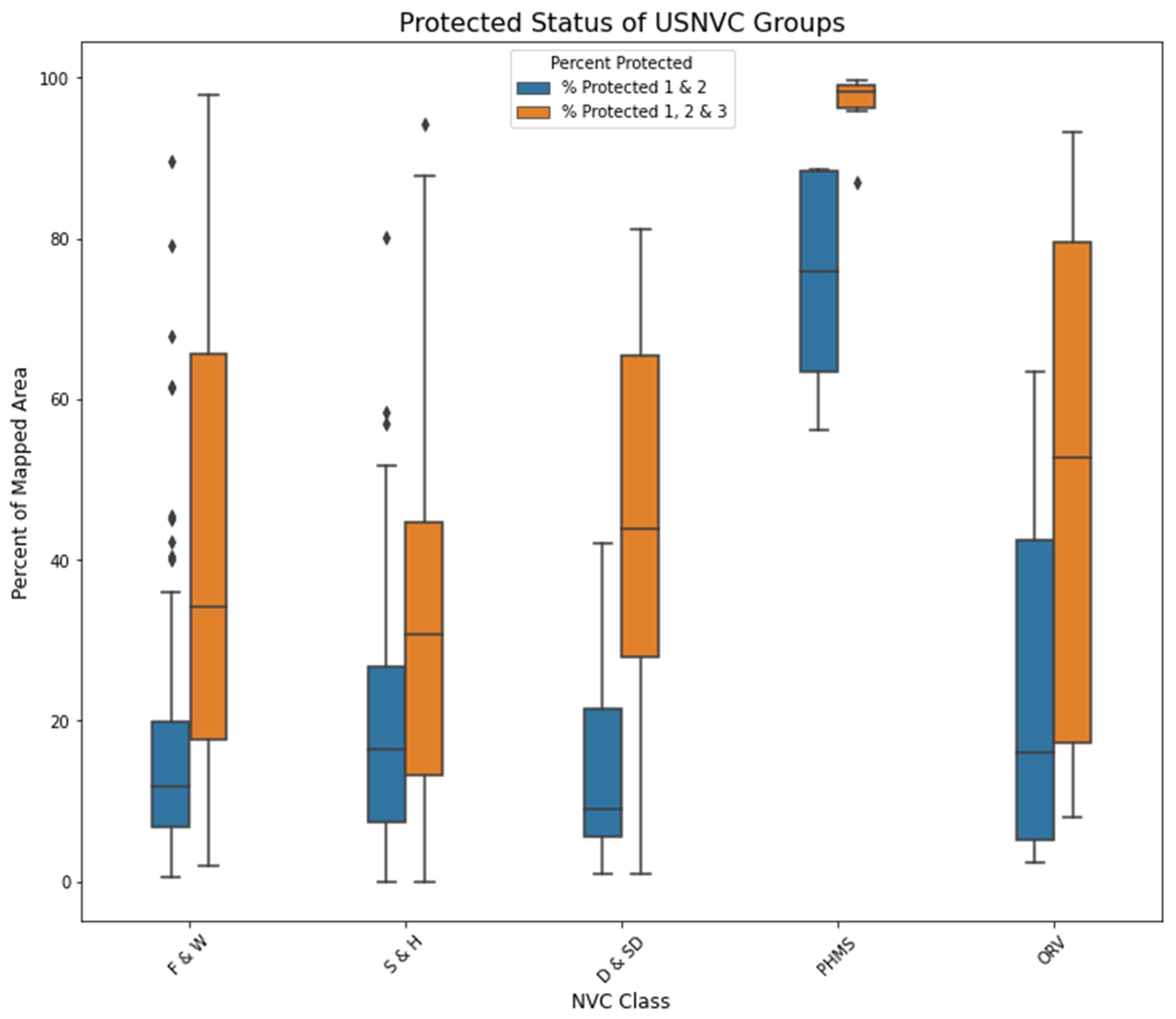
- Percent of mapped area designated protected (Status 1 & 2) and multiple use (Status 1, 2, & 3) for USNVC natural Groups across five USNVC Classes;
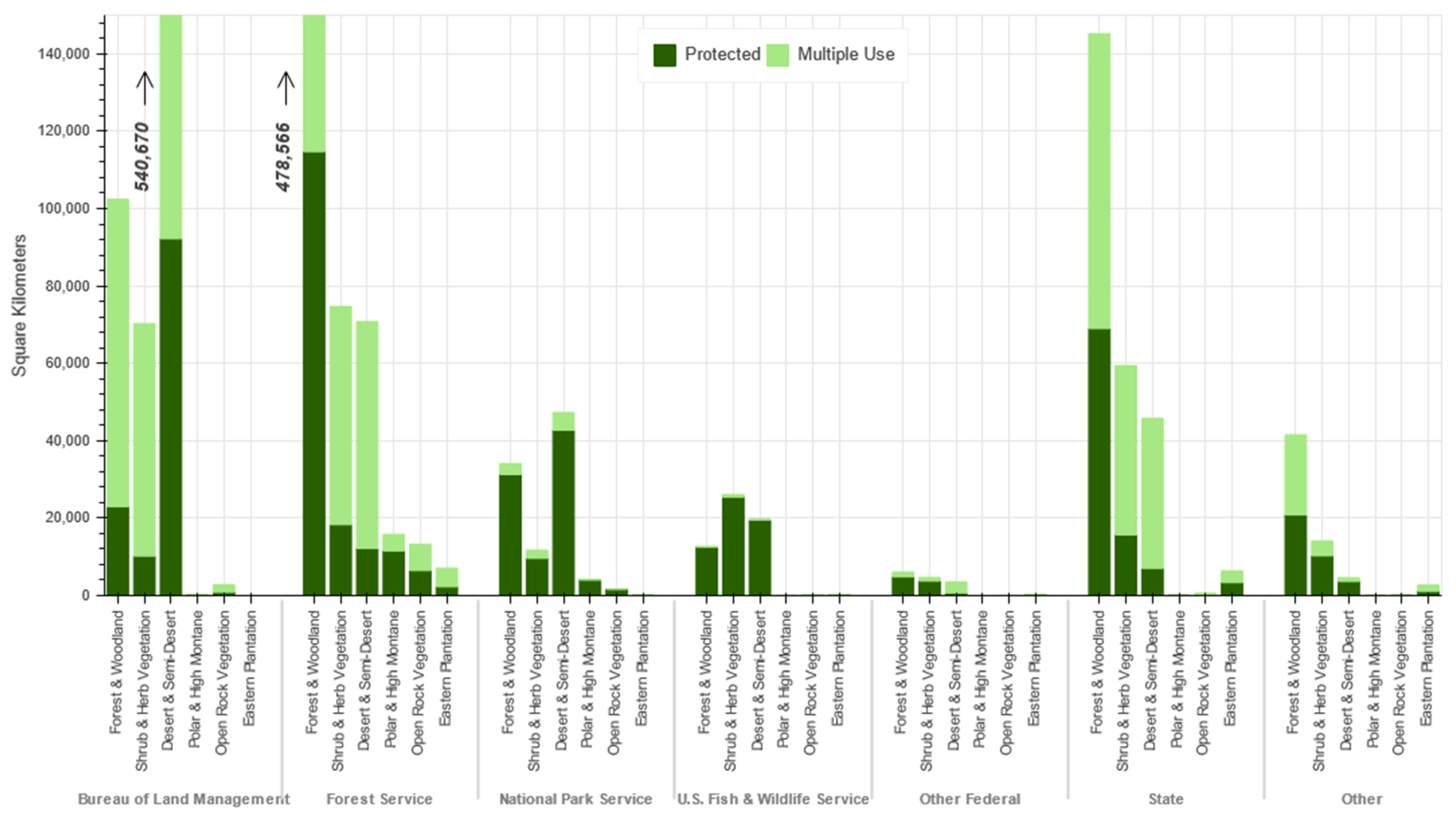
- Areal extent of protected (Status 1 & 2), and multiple use (Status 1, 2, & 3) of six USNVC Classes (natural, ruderal and plantation) by land manager (Bureau of Land Management, USDA Forest Service, National Park Service, US Fish & Wildlife Service, Other Federal, State, and Other); and
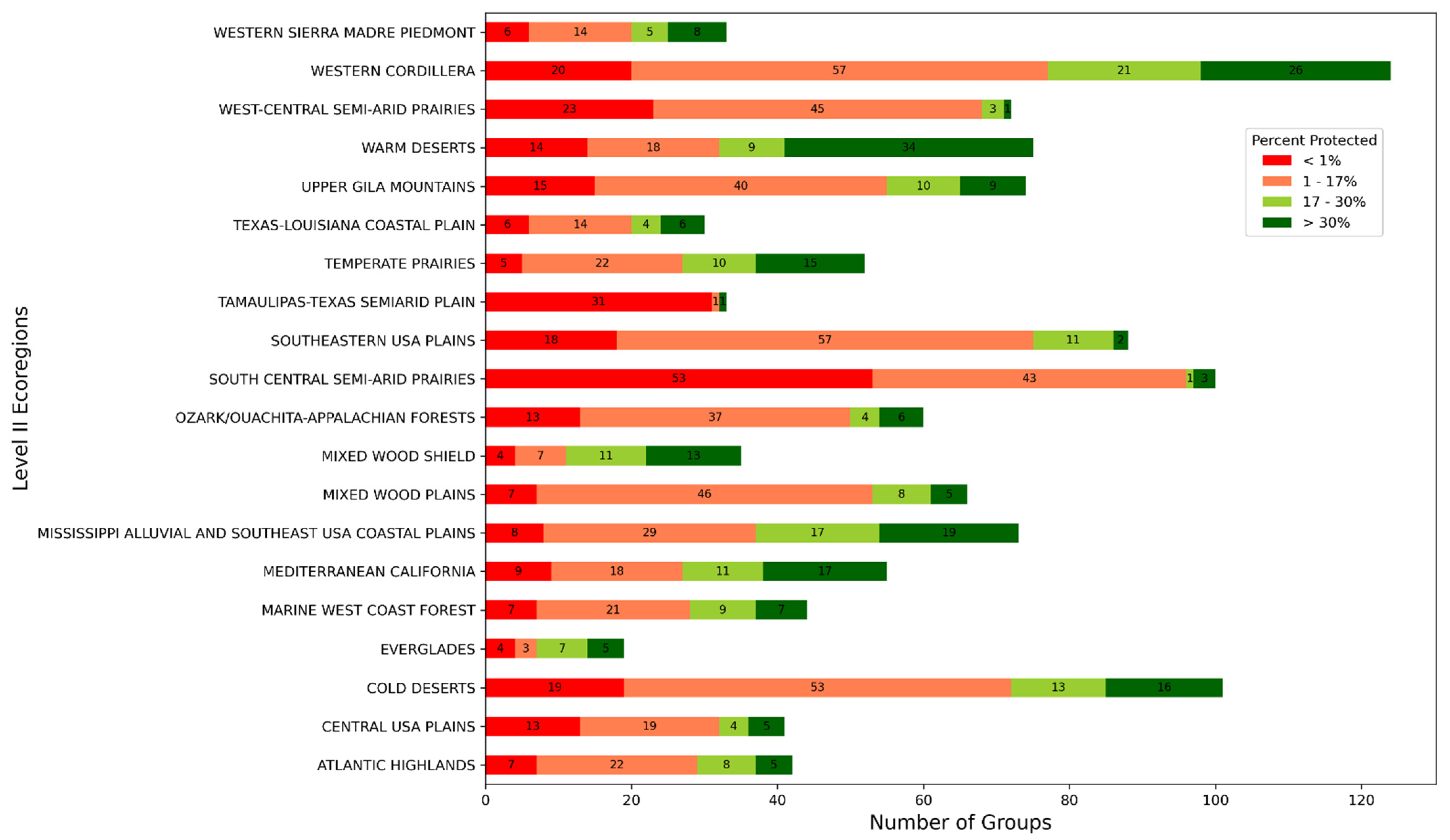
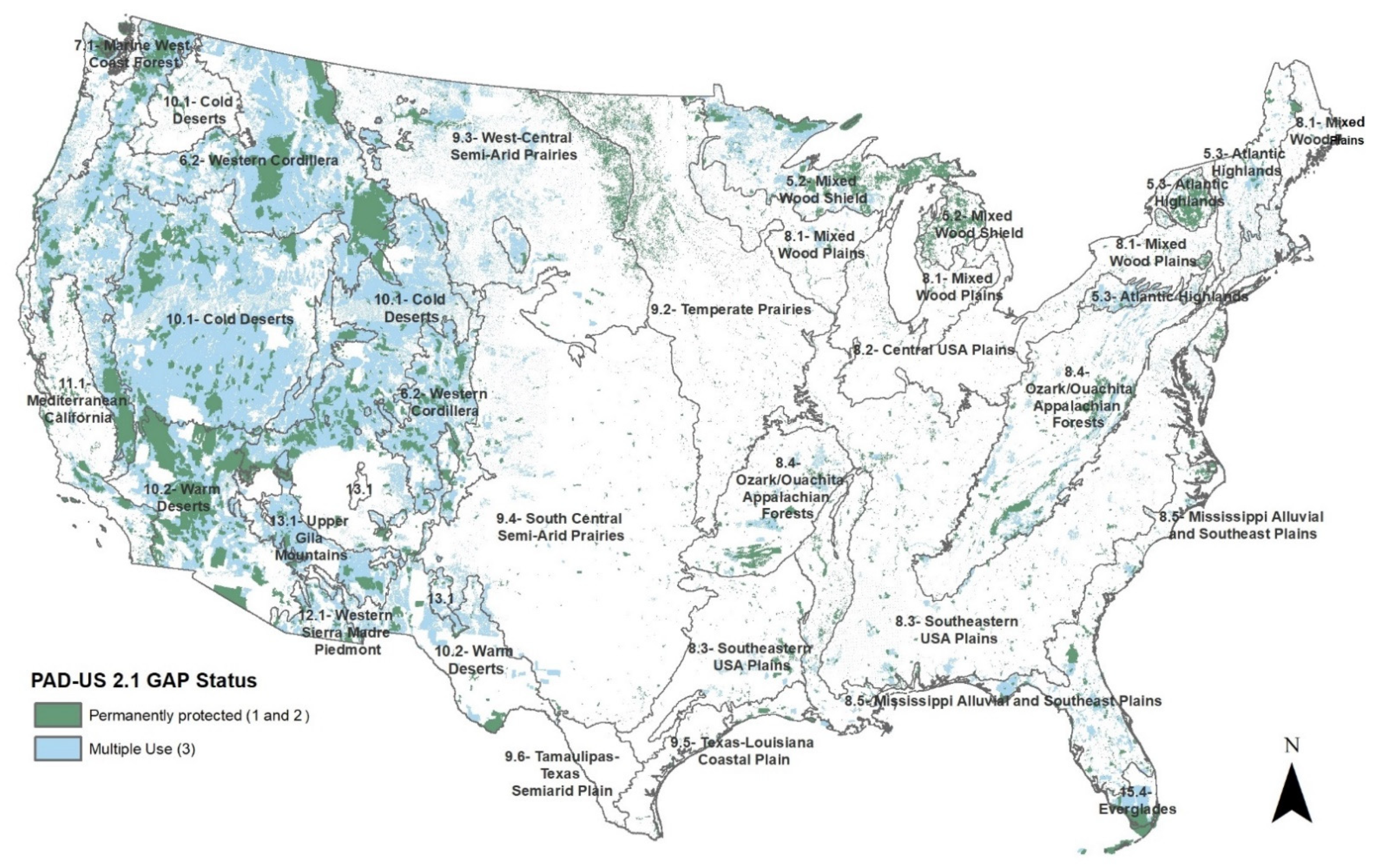
- Protection level (Status 1 & 2) of the natural USNVC Groups within four percentage categories (<1% Protected, 1–17% Protected, 17–30% Protected, >30% Protected) across Level II Ecoregions.
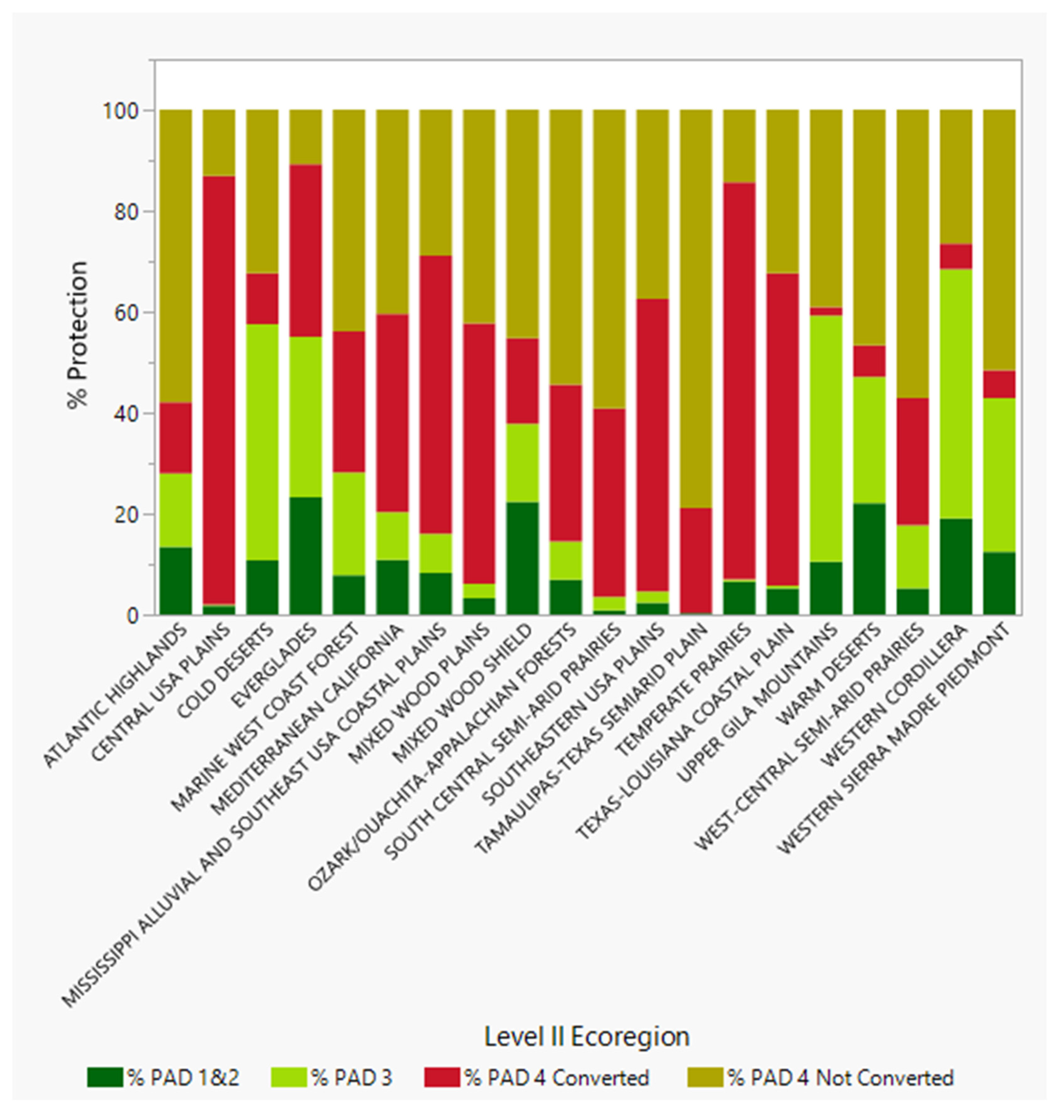
- Percentage of each Level II Ecoregion currently in Status 1 & 2 or 3 lands and the percentage Status 4 lands that has been converted to intensive uses (converted) or representing natural, ruderal or plantation vegetation (non-converted).
3. Results
3.1. Representation of Natural Groups in the Conservation Network
3.2. Spatial Patterns of Protection for USNVC Groups
3.3. Management by USNVC Class
3.4. Representation of USNVC Groups by Level II Ecoregion
3.5. Distribution of GAP Status Designation by Level II Ecoregion
4. Discussion
5. Conclusions
Supplementary Materials
Author Contributions
Funding
Data Availability Statement
Acknowledgments
Conflicts of Interest
References
- Soule, M.E. What is conservation biology? Bioscience 1985, 35, 727–734. Available online: https://www.jstor.org/stable/1310054 (accessed on 21 June 2021).
- Wu, J. Thirty years of Landscape Ecol. (1987–2017): Retrospects and prospects. Landsc. Ecol. 2017, 32, 2225–2239. [Google Scholar] [CrossRef] [Green Version]
- Myers, N. The biodiversity crisis and the future of evolution. Environmentalist 1996, 16, 37–47. [Google Scholar] [CrossRef]
- Pires, A.P.F.; Srivastava, D.S.; Marino, N.A.C.; MacDonald, A.A.M.; Figueiredo-Barros, M.P.; Farjalla, V.F. Interactive effects of climate change and biodiversity loss on ecosystem functioning. Ecology 2018, 99, 1203–1213. [Google Scholar] [CrossRef] [PubMed]
- Hooper, D.U.; Adair, E.C.; Cardinale, B.J.; Byrnes, J.E.K.; Hungate, B.A.; Matulich, K.L.; Gonzalez, A.; Duffy, J.E.; Gamfeldt, L.; O’Connor, M.I. A global synthesis reveals biodiversity loss as a major driver of ecosystem change. Nature 2012, 486, 105–108. [Google Scholar] [CrossRef]
- Trisos, C.H.; Merow, C.; Pigot, A.L. The projected timing of abrupt ecological disruption from climate change. Nature 2020, 580, 496–501. [Google Scholar] [CrossRef]
- Gotelli, N.J.; Colwell, R.K. Quantifying biodiversity: Procedures and pitfalls in the measurement and comparison of species richness. Ecol. Lett. 2001, 4, 379–391. [Google Scholar] [CrossRef] [Green Version]
- Orme, C.D.L.; Davies, R.G.; Burgess, M.; Eigenbrod, F.; Pickup, N.; Olson, V.A.; Webster, A.J.; Ding, T.-S.; Rasmussen, P.C.; Ridgely, R.S.; et al. Global hotspots of species richness are not congruent with endemism or threat. Nature 2005, 436, 1016–1019. [Google Scholar] [CrossRef]
- Laurance, W.F.; Lovejoy, T.E.; Vasconcelos, H.L.; Bruna, E.M.; Didham, R.K.; Stouffer, P.C.; Gascon, C.; Bierregaard, R.O.; Laurance, S.G.; Sampaio, E. Ecosystem decay of Amazonian forest fragments: A 22-Year Investigation. Conserv. Biol. 2002, 16, 605–618. [Google Scholar] [CrossRef] [Green Version]
- Thomas, C.D.; Cameron, A.; Green, R.E.; Bakkenes, M.; Beaumont, L.J.; Collingham, Y.C.; Erasmus, B.F.N.; de Siqueira, M.F.; Grainger, A.; Hannah, L.; et al. Extinction risk from climate change. Nature 2004, 427, 145–148. [Google Scholar] [CrossRef]
- McNeely, J. Invasive species: A costly catastrophe for native biodiversity. Land Use Water Resour. Res. 2001, 2, 1–10. [Google Scholar]
- Murray, K.A.; Retallick, R.W.R.; Puschendorf, R.; Skerratt, L.F.; Rosauer, D.; McCallum, H.I.; Berger, L.; Speare, R.; VanDerWal, J. Assessing spatial patterns of disease risk to biodiversity: Implications for the management of the amphibian pathogen, Batrachochytrium dendrobatidis. J. Appl. Ecol. 2011, 48, 163–173. [Google Scholar] [CrossRef]
- Mantyka-Pringle, C.S.; Visconti, P.; Di Marco, M.; Martin, T.G.; Rondinini, C.; Rhodes, J.R. Climate change modifies risk of global biodiversity loss due to land-cover change. Biol. Conserv. 2015, 187, 103–111. [Google Scholar] [CrossRef] [Green Version]
- Pardini, R.; Nichols, L.; Püttker, T. Biodiversity response to habitat loss and fragmentation. In Encyclopedia of the Anthropocene; DellaSalla, D., Goldstein, M., Eds.; Elsevier: Waltham, MA, USA, 2018; Volume 3, pp. 229–241. [Google Scholar] [CrossRef]
- Millennium Ecosystem Assessment. Ecosystems and Human Well-being: Biodiversity Synthesis; World Resources Institute: Washington, DC, USA, 2005; 100p. [Google Scholar]
- IUCN. Nature 2030: One Nature, One Future: A Programme for the Union 2021–2024; International Union for Conservation of Nature; World Conservation Congress: Gland, Switzerland, 2021; 24p. [Google Scholar]
- Convention on Biological Diversity. Strategic Plan for Biodiversity Including Aichi Biodiversity Targets 2011–2020; Convention on Biological Diversity: Montreal, QC, Canada, 2010. [Google Scholar]
- United States, Executive Office of the President. (Biden, J.R., Jr.). Executive Order 14008: Tackling the Climate Crisis at Home and Abroad; United States, Executive Office of the President: Washigton, DC, USA, 2021. [Google Scholar]
- National Climate Task Force. Conserving and Restoring America the Beautiful 2021. Available online: https://www.doi.gov/sites/doi.gov/files/report-conserving-and-restoring-america-the-beautiful-2021.pdf (accessed on 21 June 2021).
- Lawler, J.J.; Rinnan, D.S.; Michalak, J.L.; Withey, J.C.; Randels, C.R.; Possingham, H.P. Planning for climate change through additions to a national protected area network: Implications for cost and configuration. Philos. Trans. R. Soc. B 2020, 375, 20190117. [Google Scholar] [CrossRef] [Green Version]
- Anderson, M.G.; Ferree, C.E. Conserving the stage: Climate change and the geophysical underpinnings of species diversity. PLoS ONE 2010. [Google Scholar] [CrossRef]
- Belote, R.T.; Dietz, M.S.; Jenkins, C.N.; McKinley, P.S.; Irwin, G.H.; Fullman, T.J.; Leppi, J.C.; Aplet, G.H. Wild, connected, and diverse: Building a more resilient system of protected areas. Ecol. Appl. 2017, 27, 1050–1056. [Google Scholar] [CrossRef]
- Scott, J.M.; Davis, F.W.; McGhie, R.G.; Wright, R.G.; Groves, C.; Estes, J. Nature reserves: Do they capture the full range of america’s biological diversity? Ecol. Appl. 2001, 11, 999–1007. [Google Scholar] [CrossRef]
- Scott, J.M.; Davis, F.; Csuti, B.; Noss, R.; Butterfield, B.; Groves, C.; Anderson, H.; Caicco, S.; D’Erchia, F.; Edwards, T.C., Jr.; et al. Gap analysis: A geographic approach to protection of biological diversity. Wildl. Monogr. 1993, 123, 3–41. [Google Scholar]
- Davidson, A.; Dunn, L.; Gergely, K.; McKerrow, A.; Williams, S.; Case, M. Refining the coarse filter approach: Using habitat-based species models to identify rarity and vulnerabilities in the protection of U.S. biodiversity. Glob. Ecol. Conserv. 2021. [Google Scholar] [CrossRef]
- Gould, W.A.; Alarcón, C.; Fevold, B.; Jiménez, M.E.; Martinuzzi, S.; Potts, G.; Quiñones, M.; Solórzano, M.; Ventosa, E. The Puerto Rico Gap Analysis Project. Volume 1: Land Cover, Vertebrate Species Distributions, and Land Stewardship; Gen. Tech. Rep. IITF-GTR-39; U.S. Department of Agriculture, Forest Service, International Institute of Tropical Forestry: Río Piedras, Puerto Rico, 2008; 165p. [Google Scholar]
- Gon, S.M., III; Allison, A.; Cannarella, R.J.; Jacobi, J.D.; Kaneshiro, K.Y.; Kido, M.H.; Lane-Kamahele, M.; Miller, S.E. The Hawai‘i GAP Analysis Final Report; Report, U.S. Department of Interior, U.S. Geological Survey: Washigton, DC, USA, 2006; 162p. [Google Scholar]
- Boykin, K.G.; Stoner, L.L.; Lowry, J.H.; Schrupp, D.L.; Bradford, D.F.; O’Brien, L.; Thomas, K.A.; Drost, C.; Ernst, A.E.; Kepner, W.J.; et al. Analysis based on stewardship and management status. In Southwest Regional Gap Analysis Final Report; U.S. Geological Survey, Gap Analysis Program: Washington, DC, USA, 2007; Chapter 5. [Google Scholar]
- Aycrigg, J.L.; Davidson, A.; Svancara, L.K.; Gergely, K.J.; McKerrow, A.J.; Scott, J.M. Representation of ecological systems within the protected areas network of the continental United States. PLoS ONE 2013, 8, e54689. [Google Scholar] [CrossRef] [Green Version]
- Whittaker, R.H. Communities and Ecosystems, 2nd ed.; MacMillan: New York, NY, USA, 1975; p. 385. [Google Scholar]
- Franklin, J.F. Preserving Biodiversity: Species, Ecosystems, or Landscapes? Ecol. Appl. 1993, 3, 202–205. [Google Scholar] [CrossRef] [PubMed] [Green Version]
- Noss, R.F. Indicators for monitoring biodiversity: A hierarchical approach. Conserv. Biol. 1990, 4, 355–364. [Google Scholar] [CrossRef]
- Gergely, K.J.; Boykin, K.G.; McKerrow, A.J.; Rubino, M.J.; Tarr, N.M.; Williams, S.G. Gap Analysis Project (GAP) Terrestrial Vertebrate Species Richness Maps for the Conterminous U.S.; U.S. Geological Survey Scientific Investigations Report 2019–5034; Gap Analysis Program: Washington, DC, USA, 2019; 99p. [Google Scholar] [CrossRef] [Green Version]
- Franklin, S.; Faber-Langendoen, D.; Jenning, S.M.; Keeler-Wolf, T.; Loucks, O.; Peet, R.; Roberts, D.; McKerrow, A. Building the United States national vegetation classification. Ann. Bot. 2012, 2, 1–9. [Google Scholar]
- Eyre, F.H. Forest Cover Types of the United States and Canada; Society of American Foresters: Washington, DC, USA, 1980; p. 148. [Google Scholar]
- Cowardin, L.M.; Carter, V.; Golet, F.C.; LaRoe, E.T. Classification of Wetlands and Deepwater Habitats of the United States; FWS/OBS-79/31; U.S. Fish and Wildlife Service: Washington, DC, USA, 1979. [Google Scholar]
- Brown, D.E. Biotic Communities of the American Southwest-United States and Mexico. Desert Plants 1982, 4, 1–342. [Google Scholar]
- Madden, M.; Jones, D.; Vilchek, L. Photointerpretation key for the Everglades Vegetation Classification System. Photogramm. Eng. Remote Sens. 1999, 65, 171–177. [Google Scholar]
- Brown, D.E. A system for classifying cultivated and cultured lands within a systematic classification of natural ecosystems. J. Ariz. Nev. Acad. Sci. 1980, 15, 4853. Available online: https://www.jstor.org/stable/40024073 (accessed on 21 June 2021).
- Anderson, R.J.; Hardy, E.E.; Roach, J.T.; Witmer, R.E. A Land Use and Land Cover Classification System for Use with Remote Sensor Data; U.S. Geological Survey Professional Paper 964; U.S. Geological Survey: Washigton, DC, USA, 1976; 28p. [Google Scholar]
- Federal Geographic Data Committee. Vegetation Subcommittee. Vegetation Classification Standard; FGDC-STD-005; U.S. Geological Survey, Federal Geographic Data Committee, Vegetation Subcommittee: Reston, VA, USA, 1997. Available online: http://www.fgdc.gov/standards/documents/standards/vegetation/vegclass.pdf (accessed on 21 June 2021).
- Federal Geographic Data Committee. Vegetation Subcommittee. National Vegetation Classification Standard, Version 2; FGDC-STD-005-2008; Federal Geographic Data Committee, U.S. Geological Survey: Reston, VA, USA, 2008. Available online: http://www.fgdc.gov/standards/documents/standards/vegetation/vegclass.pdf (accessed on 21 June 2021).
- Faber-Langendoen, D.; Keeler-Wolf, T.; Meidinger, D.; Tart, D.; Hoagland, B.; Josse, C.; Navarro, G.; Ponomarenko, S.; Saucier, J.-P.; Weakley, A.; et al. EcoVeg: A new approach to vegetation description and classification. Ecol. Monogr. 2014, 84, 533–561. [Google Scholar] [CrossRef]
- Faber-Langendoen, D.; Keeler-Wolf, T.; Meidinger, D.; Josse, C.; Weakley, A.; Tart, D.; Navarro, G.; Hoagland, B.; Ponomarenko, S.; Fults, G.; et al. Classification and Description of World Formation Types; Gen. Tech. Rep. RMRS-GTR-346; U.S. Department of Agriculture, Forest Service, Rocky Mountain Research Station: Fort Collins, CO, USA, 2016; 222p. [Google Scholar]
- Comer, P.; Faber-Langendoen, D.; Evans, R.; Gawler, S.; Josse, C.; Kittel, G.; Menard, S.; Pyne, M.; Reid, M.; Schulz, K.; et al. Ecological Systems Of The United States: A Working Classification of U.S. Terrestrial Systems; NatureServe: Arlington, VA, USA, 2003. [Google Scholar]
- U.S. Geological Survey (USGS) Gap Analysis Project (GAP), 2020. Protected Areas Database of the United States (PAD-US) 2.1: U.S. Geological Survey Data Release. Available online: https://doi.org/10.5066/P92QM3NT (accessed on 21 June 2021).
- Picotte, J.J.; Dockter, D.; Long, J.; Tolk, B.; Davidson, A.; Peterson, B. LANDFIRE Remap Prototype Mapping Effort: Developing a New Framework for Mapping Vegetation Classification, Change, and Structure. Fire 2019, 2, 35. [Google Scholar] [CrossRef] [Green Version]
- Dockter, D.; Callahan, K.; Tolk, B.; Peterson, B. LANDFIRE Remap: Improvements in national ecosystem modeling and vegetation mapping. In Proceedings of the Ecological Society of America Annual Meeting, Virtual Meeting, 3–6 August 2020. [Google Scholar]
- Nelson, K.J.; Steinwand, D. A Landsat data tiling and compositing approach optimized for change detection in the conterminous United States. Photogramm. Eng. Remote Sens. 2015, 81, 13–26. [Google Scholar] [CrossRef]
- Yang, L.; Jin, S.; Danielson, P.; Homer, C.; Gass, L.; Bender, S.M.; Case, A.; Costello, C.; Dewitz, J.; Fry, J.; et al. A new generation of the United States National Land Cover Database: Requirements, research priorities, design, and implementation strategies. ISPRS J. Photogramm. Remote Sens. 2018, 146, 108–123. [Google Scholar] [CrossRef]
- Boryan, C.; Yang, Z.; Mueller, R.; Craig, M. Monitoring US agriculture: The US Department of Agriculture, National Agricultural Statistics Service, Cropland Data Layer Program. Geocarto Int. 2011, 26, 341–358. [Google Scholar] [CrossRef]
- Caratti, J.F. The LANDFIRE prototype project reference database. In The LANDFIRE Prototype Project: Nationally Consistent and Locally Relevant Geospatial Data for Wildland Fire Management; Rollins, M.G., Frame, C., Eds.; Gen. Tech. Rep. RMRS-GTR-175; Department of Agriculture, Forest Service Rocky Mountain Research Station: Fort Collins, CO, USA, 2006; pp. 69–98. [Google Scholar]
- LANDFIRE. USGS Earth Resources Observation and Science Center (EROS), U.S. Geological Survey. LANDFIRE Remap 2016 National Vegetation Classification (NVC) CONUS. 2020. Available online: https://www.landfire.gov (accessed on 24 February 2021).
- Environmental Systems Research Institute. ArcGIS 10.7 Spatial Analyst Toolbox. What is the ArcGIS Spatial Analyst Extension?—ArcGIS Help|Documentation. Available online: https://desktop.arcgis.com/en/arcmap/10.7/tools/spatial-analyst-toolbox/an-overview-of-the-spatial-analyst-toolbox.htm (accessed on 21 June 2021).
- Omernik, J.M.; Griffith, G.E. Ecoregions of the conterminous United States: Evolution of a hierarchical spatial framework. Environ. Manag. 2014, 54, 1249–1266. [Google Scholar] [CrossRef]
- Faber-Langendoen, D.; Baldwin, K.; Keeler-Wolf, T.; Meidinger, D.; Muldavin, E.; Peet, R.K.; Josse, C. The EcoVeg Approach in the Americas: U.S., Canadian, and International Vegetation Classifications. Phytocoenologia 2018, 48, 215–237. [Google Scholar] [CrossRef]
- Lea, C. Vegetation Classification Guidelines: National Park Service Vegetation Inventory, Version 2.0. 2001; Natural Resource Report NPS/NRPC/NRR—2011/374; National Park Service: Fort Collins, CO, USA, 2021. [Google Scholar]
- Hak, J.C.; Patrick, J.; Comer, P.J. Modeling landscape condition for biodiversity assessment—Application in temperate North America. Ecol. Ind. 2017, 82, 206–216. [Google Scholar] [CrossRef]
- Aycrigg, J.L.; Tricker, J.; Travis Belote, R.; Dietz, M.S.; Duarte, L.; Aplet, G.H. The Next 50 Years: Opportunities for Diversifying the Ecological Representation of the National Wilderness Preservation System within the Contiguous United States. J. For. 2016, 114, 396–404. [Google Scholar] [CrossRef]
- NatureServe. The Status of Biodiversity in the United States; NatureServe: Arlington, VA, USA, 2021. [Google Scholar]
- Jenkins, C.; Van Houtan, K.; Pimm, S.; Sexton, J. US protected lands mismatch biodiversity priorities. Proc. Natl. Acad. Sci. USA 2015, 112, 5081–5086. [Google Scholar] [CrossRef] [Green Version]


| NVC Level | Vegetation Criteria | Ecological Criteria | Scientific Name | Colloquial Name |
|---|---|---|---|---|
| UPPER LEVELS | PREDOMINANT PHYSIOGNOMY | |||
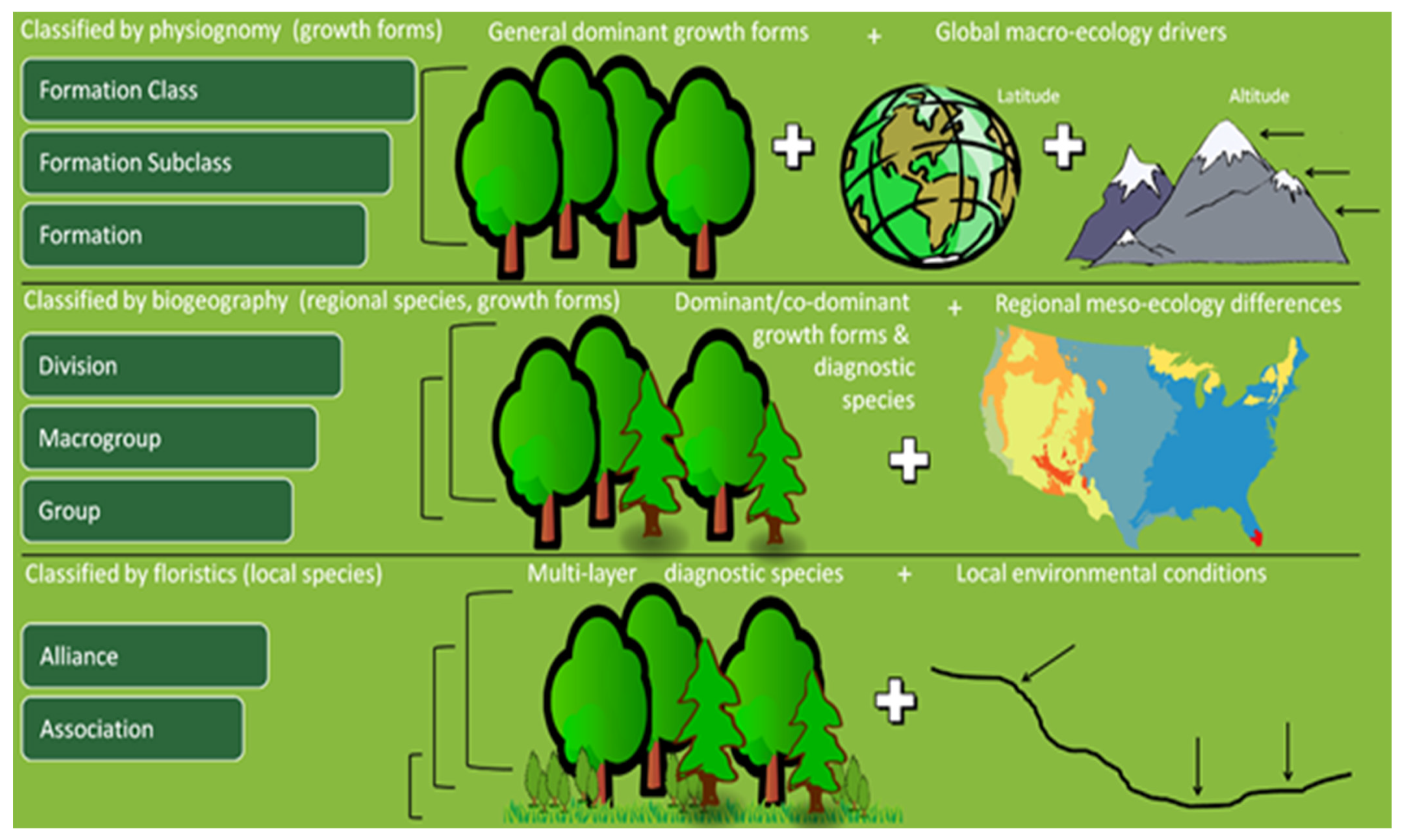
| 1 Formation Class | Broad combinations of general dominant growth forms | Basic temperature (energy budget), moisture and substrate/aquatic conditions. | Mesomorphic Tree Vegetation Class | Forest & Woodland |
| 2 Formation Subclass | Combinations of general dominant and diagnostic growth forms. | Global macroclimatic factors driven primarily by latitude and continental position or overriding substrate/aquatic conditions | Temperate & Boreal Forest & Woodland Subclass | Temperate & Boreal Forest & Woodland |
| 3 Formation | Combinations of dominant and diagnostic growth forms. | Global macroclimatic factors as modified by altitude, seasonality of precipitation, substrates and hydrologic conditions. | Cool Temperate Forest & Woodland Formation | Cool Temperate Forest & Woodland |
| MIDDLE LEVELS | PHYSIOGNOMY, BIOGEOGRAPHY AND FLORISTICS. | |||
| 4 Division | Combinations of dominant and diagnostic growth forms and a broad set of diagnostic plant species that reflect biogeographic differences. | Continental differences in mesoclimate, geology, substrates, hydrology and disturbance regimes. | Douglas-fir—Western Hemlock—Subalpine Fir Forest & Woodland Division | Rocky Mountain Forest & Woodland |
| 5 Macrogroup | Combinations of moderate sets of diagnostic plant species and diagnostic growth forms that reflect biogeographic differences. | Sub-continental to regional differences in mesoclimate, geology, substrates, hydrology, and disturbance regimes. | Subalpine Fir—Engelmann Spruce—Whitebark Pine Rocky Mountain Forest Macrogroup | Rocky Mountain Subalpine-High Montane Forest |
| 6 Group | Combinations of relatively narrow sets of diagnostic plant species, including dominants and co-dominants, broadly similar composition and diagnostic growth forms. | Regional mesoclimate, geology, substrates, hydrology and disturbance regimes. | Engelmann Spruce—Subalpine Fir—Mountain Hemlock Moist Forest & Woodland Group | Rocky Mountain Subalpine Moist Spruce—Fir Forest & Woodland |
| LOWER LEVELS | PREDOMINANTLY FLORISTICS | |||
| 7 Alliance | Diagnostic species, including some from the dominant growth form or layer, and moderately similar composition. | Regional to subregional climate, substrates, hydrology, moisture/nutrient factors and disturbance regimes. | Subalpine Fir—Quaking Aspen Rocky Mountain Moist Forest Alliance | Rocky Mountain Moist Subalpine Fir—Aspen Forest |
| 8 Association | Diagnostic species, usually from multiple growth forms or layers, and more narrowly similar composition. | Topo-edaphic climate, substrates, hydrology, and disturbance regimes. | Quaking Aspen— Subalpine Fir/Tall Forbs Forest | Quaking Aspen— Subalpine Fir/Tall Forbs Forest |
| Status | Criteria and Examples |
|---|---|
| 1 | An area having permanent protection from conversion of natural land cover and a mandated management plan in operation to maintain a natural state within which disturbance events (of natural type, frequency, intensity, and legacy) are allowed to proceed without interference or are mimicked through management. National Parks, Wilderness Areas |
| 2 | An area having permanent protection from conversion of natural land cover and a mandated management plan in operation to maintain a primarily natural state, but which may receive uses or management practices that degrade the quality of existing natural communities, including suppression of natural disturbance. National Wildlife Refuges, State Parks, The Nature Conservancy Preserves |
| 3 | An area having permanent protection from conversion of natural land cover for the majority of the area, but subject to extractive uses of either a broad, low-intensity type (e.g., logging, Off Highway Vehicle recreation) or localized intense type (e.g., mining). It also confers protection to federally listed endangered and threatened species throughout the area. National Forests, BLM Lands, State Forests, some State Parks |
| 4 | There are no known public or private institutional mandates or legally recognized easements or deed restrictions held by the managing entity to prevent conversion of natural habitat types to anthropogenic habitat types. The area generally allows conversion to unnatural land cover throughout or management intent is unknown. Unknown areas, private lands, developed or agriculture areas |
Publisher’s Note: MDPI stays neutral with regard to jurisdictional claims in published maps and institutional affiliations. |
© 2021 by the authors. Licensee MDPI, Basel, Switzerland. This article is an open access article distributed under the terms and conditions of the Creative Commons Attribution (CC BY) license (https://creativecommons.org/licenses/by/4.0/).
Share and Cite
McKerrow, A.; Davidson, A.; Rubino, M.; Faber-Langendoen, D.; Dockter, D. Quantifying the Representation of Plant Communities in the Protected Areas of the U.S.: An Analysis Based on the U.S. National Vegetation Classification Groups. Forests 2021, 12, 864. https://doi.org/10.3390/f12070864
McKerrow A, Davidson A, Rubino M, Faber-Langendoen D, Dockter D. Quantifying the Representation of Plant Communities in the Protected Areas of the U.S.: An Analysis Based on the U.S. National Vegetation Classification Groups. Forests. 2021; 12(7):864. https://doi.org/10.3390/f12070864
Chicago/Turabian StyleMcKerrow, Alexa, Anne Davidson, Matthew Rubino, Don Faber-Langendoen, and Daryn Dockter. 2021. "Quantifying the Representation of Plant Communities in the Protected Areas of the U.S.: An Analysis Based on the U.S. National Vegetation Classification Groups" Forests 12, no. 7: 864. https://doi.org/10.3390/f12070864
APA StyleMcKerrow, A., Davidson, A., Rubino, M., Faber-Langendoen, D., & Dockter, D. (2021). Quantifying the Representation of Plant Communities in the Protected Areas of the U.S.: An Analysis Based on the U.S. National Vegetation Classification Groups. Forests, 12(7), 864. https://doi.org/10.3390/f12070864