Article

New Representation of Plant Hydraulics Improves the Estimates of Transpiration in Land Surface Model

1
Southern Marine Science and Engineering Guangdong Laboratory (Zhuhai), Guangdong Province Key Laboratory for Climate Change and Natural Disaster Studies, School of Atmospheric Sciences, Sun Yat-sen University, Guangzhou 510275, China
2
Key Laboratory of Meteorological Disaster, Ministry of Education/International Joint Research Laboratory of Climate and Environment Change/Collaborative Innovation Center on Forecast and Evaluation of Meteorological Disasters, Nanjing University of Information Science & Technology (NUIST), Nanjing 210044, China
3
School of Atmospheric Sciences, Nanjing University of Information Science and Technology, Nanjing 210044, China
*
Author to whom correspondence should be addressed.
Forests 2021, 12(6), 722; https://doi.org/10.3390/f12060722
Submission received: 3 April 2021 / Revised: 19 May 2021 / Accepted: 25 May 2021 / Published: 1 June 2021
(This article belongs to the Section Forest Ecophysiology and Biology)

Abstract

:
Transpiration represents more than 30% of the global land–atmosphere water exchange but is highly uncertain. Plant hydraulics was ignored in traditional land surface modeling, but recently plant hydraulics has been found to play an essential role in transpiration simulation. A new physical-based representation of plant hydraulic schemes (PHS) was recently developed and implemented in the Common Land Model (CoLM). However, it is unclear to what extent PHS can reduce these uncertainties. Here, we evaluated the PHS against measurements obtained at 81 FLUXNET sites. The transpiration of each site was estimated using an empirical evapotranspiration partitioning approach. The metric scores defined by the International Land Model Benchmarking Project (ILAMB) were used to evaluate the model performance and compare it with that of the CoLM default scheme (soil moisture stress (SMS)). The bias score of transpiration in PHS was higher than SMS for most sites, and more significant improvements were found in semi-arid and arid sites where transpiration was limited by soil moisture. The hydraulic redistribution in PHS optimized the soil water supply and thus improved the transpiration estimates. In humid sites, no significant improvement in seasonal or interannual variability of transpiration was simulated by PHS, which can be explained by the insensitivity of transpiration demand coupled to the photosynthesis response to precipitation. In arid and semi-arid sites, seasonal or interannual variability of transpiration was better captured by PHS than SMS, which was interpreted by the improved drought sensitivity for transpiration. Arid land is widespread and is expected to expand due to climate change, thus there is an urgent need to couple PHS in land surface models.

1. Introduction

Globally, transpiration accounts for 30% of the land–atmosphere water exchange, or 60% (mean ± 1 standard deviation (s.d.)) of continental evapotranspiration [1,2]. The transpiration proportion of evapotranspiration is related to an important scientific question of how to dominate the biotic contribution in the land–atmosphere water exchange [3]. In recent decades, agriculturalists, ecologists, and climate change researchers have put great effort into understanding and improving the evapotranspiration partitioning estimates [4,5,6,7]. Several approaches have been developed to estimate evapotranspiration partitioning at large spatial scales. For example, isotope data have been used to estimate the percentage of transpiration in evapotranspiration [5]. Wei et al. [2] have built up empirical relationships between leaf area index (LAI) and transpiration for different vegetation types using satellite data and model estimation results. Both approaches have represented large-scale transpiration partitioning well with reliable technical theories.
Process-based models have been recently used to partition evapotranspiration as well. Land surface models, one of the most robust large-scale flux estimation tools so far, estimate transpiration, soil evaporation, and canopy interception based on plant physiological processes, canopy physical processes, and soil hydrological processes. However, many land surface models have been found to underestimate the transpiration component of evapotranspiration significantly. For instance, GSWP-2 (the Global Soil Wetness Project 2) estimates transpiration comprises 48% of evapotranspiration [8]. The global transpiration partitioning estimated by CLM (the Community Land Model) has a mean value of about 49% (CLM3: 41%, CLM3.5: 43%, CLM4CN: 56%, CLM4CNE: 56%, CLM4SP: 48%) [9,10]. Yoshimura et al. [11] attributed about 29% of land evapotranspiration (ET) to transpiration (T) based on Iso-Matsiro. Wang-Erlandsson et al. [12] reported that STEAM (Simple Terrestrial Evaporation to Atmosphere Model) estimates a mean global terrestrial evaporation of 73,900 km3 year−1, of which 59% is transpiration. Most of these fractions from process-based models are significantly lower than observations.
Previous studies have indicated that underestimating modeled transpiration maybe is not the only, but probably one of the most important reasons for the lower-than-expected transpiration fractions [10]. Soil water stress is the major constraint on modeled transpiration through stomatal behavior; however, most soil water stress schemes are empirically parameterized in land surface models [13]. The development of a plant hydraulic module improves the representation of the plant water transport in the model. The physically-based plant hydraulic stress (PHS) scheme replaces the empirically-based soil moisture stress (SMS) parameterization in describing the physiological response to drought [14]. The hydraulic redistribution (HR) scheme refers to the passive water movement via plant roots from relatively moist to dry soil. The HR schemes are supported by many field experiments and scientific literature [15,16,17]. Ryel et al. [18] has developed the soil layer connection model to represent HR, which calculates HR water flux according to soil water potential in separate layers. However, the flows within the root system are not considered in Ryel’s HR model. Amenu and Kumar [19] have incorporated radial water flow, and axial water flow into the root system and, therefore, represent more realistic HR processes. Community land Model Version 5 (CLM5) has incorporated PHS and represents HR as a natural consequence of Darcy’s Law implementation [14]. Much effort has been expended into developing HR models. However, the absence of direct measurements on transpiration prevents the comprehensive evaluation of the plant hydraulic module.
A global database of plant sap flow measurement, SAPFLUXNET, has been widely used to understand ecological factors driving plant transpiration and evaluate land surface models [20]. Although the SAPFLUXNET dataset provides direct measurements on transpiration from over 120 sites worldwide, the modeled transpiration at the stand level cannot be directly compared with the sap flow measurement of individual plants. Upscaling from the individual to the stand level may introduce additional uncertainties [20]. The FLUXNET dataset is the most frequently used for the analysis of stand-level measurements, including land-atmosphere flux measurements from more than 900 sites [21]. However, FLUXNET data only provide latent heat or evapotranspiration as the land-atmosphere water flux. Transpiration from the plant hydraulic module cannot be directly evaluated against FLUXNET data. Alternatively, the empirical evapotranspiration partitioning approach proposed by Wei et al. [2] has been well-validated, and is widely used in estimating large-scale, grid-based transpiration.
Here, we evaluated the modeled transpiration against the observation-based estimates of transpiration from 81 FLUXNET sites, and the specific information of each site is given in Table S1. We conducted Common Land Model (CoLM) simulations with the PHS scheme and the SMS scheme at each site, respectively. The simulated transpiration was compared with that derived from the empirical evapotranspiration partitioning approach [2]. Two metrics (the bias score and the root mean square error (RMSE) score) from the International Land Model Benchmarking (ILAMB) system were used to evaluate the overall average and the variability of the modeled transpiration. We aimed to answer whether or how much the plant hydraulic module in land surface models improves modeled transpiration. Can we identify what mechanisms the plant hydraulic module improves?

2. Materials and Methods

2.1. Model Description

We evaluate the transpiration modeled by CoLM PHS. The current release version CoLM2014 is developed from an initial version of CoLM [22]. CoLM is a process-based land surface model that includes soil thermal, soil hydrology, plant physiological, canopy radiation, turbulence, and other processes [23,24]. The CoLM PHS employs a fine representation of plant hydraulics. The root water potential is calculated at 10 different depths, equivalent to the number of soil layers. Meanwhile, the numerical scheme for plant water stress was significantly simplified. The new numerical scheme solves the stomatal conductance, plant water potential, and water stress within the same iteration, whereas CLM5 PHS solves them in three nested iterations; 86% of computational cost is saved by the new numerical scheme in the plant physiological module.
The CoLM PHS calculates transpiration based on the concept of the soil–plant–atmosphere continuum (SPAC). The plant water transport in the CoLM PHS is driven by the water potential gradient from soil to leaves. The above vegetation water potentials are solved at four aboveground vegetation nodes, including sunlit leaf, shaded leaf, stem, and root at the soil surface. The water transport between two adjacent nodes follows Darcy’s law, which is commonly used in plant hydraulic scheme of land surface models [14]:
q i j = k i j ( Ψ i Ψ j )
where q i j is water transport from j node to i node, and k i j is hydraulic conductance between j node and i node. Ψ i and Ψ j are water potential at i node and j node, respectively. Transpiration of the sun leaf and shaded leaf can be derived by q l e a f s t e m ( s u n l e a f , s h a l e a f ) . The vegetation water transport from belowground is divided into axial and radial solutions. In the radial solution, water is transferred between the soil and root.
The variation in plant and soil water potential in PHS is governed by three plant hydraulic processes: plant embolization, HR, and stomatal water response. The plant embolization process represents the reduction in hydraulic conductivity when plant water potential declines due to drought. A transpiration attenuation function, which represents the stomata response to water stress [25] and the vulnerability curve of hydraulic conductance [14], was introduced into PHS to depict the plant embolization process, which is missing in SMS.
The HR process describes the vertical water transport through the root system, and HR usually moves water downward during the wet season and lifts water upward during the dry season. In SMS, root water uptake of each layer only depends on the dimensionless ratio of each layer of the root. In PHS, the root water uptake is determined by the water potential difference between the soil and root in each layer so that the HR process can be represented.
The stomatal response process parameterizes the stomata conductance changes in response to drought. Leaf water potential as a physical-based variable is used to quantify the plant water stress on stomatal conductance. Plant water stress is described by a water stress factor, which constrains the water response in photosynthesis and transpiration. In SMS, the water stress factor is empirically determined by soil water potential, while in PHS, it depends on leaf water potential, which directly represents the relationship to stomata conductance reduction [25]. The specific solution of PHS is given in Appendix A and Appendix B.

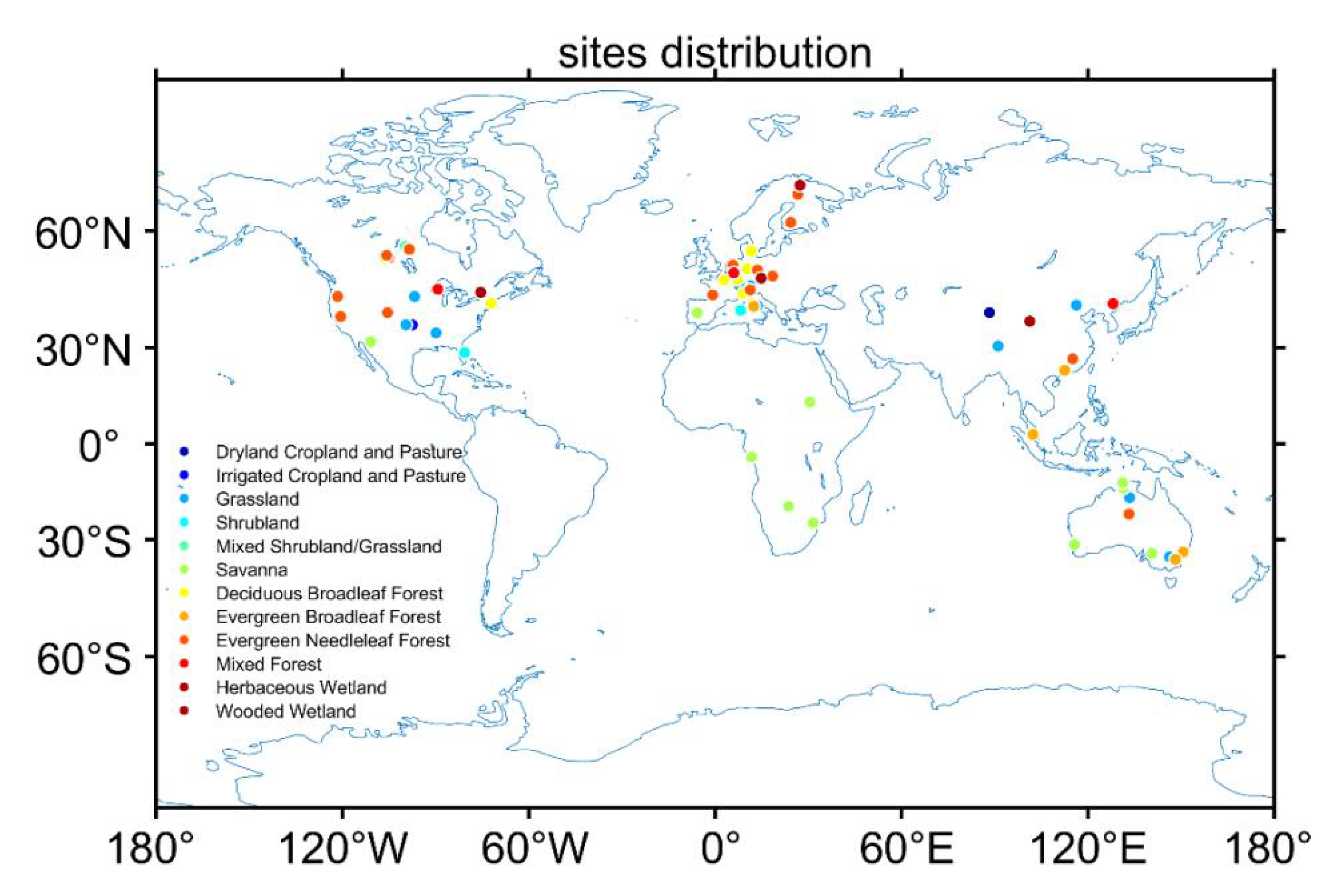
2.2. Forcing Data from FLUXNET Observations

We used half-hourly data for eight observed atmospheric forcing variables from the FLUXNET2015 Dataset (https://FLUXNET.fluxdata.org/data/FLUXNET2015-dataset/ (accessed on 21 May 2020)) as the model input, which included downward solar radiation at the surface (W m−2), downward longwave radiation (W m−2), precipitation (mm s−1), temperature at the reference height (K), wind speed (u, v) (m s−1), atmospheric pressure at the surface (Pa), and specific humidity at the reference height (kg kg−1).
To improve the accuracy of the evaluation, we use the quality control results of the latent heat flux. Quality control results from 56 sites were given by FLUXNET directly, and the missing data were filled using uncorrected latent heat flux. For the remaining sites for which the quality control results were not given directly, we used the following tuning equations to resolve the imbalance issue of the surface energy budgets [26]:
H L , c o r = A   H L , u = R n e t H G H S , u + H L , u H L , u
where the variables with the subscript cor indicate the corrected variables, and u means the uncorrected variables. HL,cor is the corrected latent heat flux, which we use as the quality control result. HL,u is the uncorrected latent heat flux. HS,u is the uncorrected sensible heat flux. Rnet and HG are the net solar radiation and ground heat flux, respectively. HG is a direct measurement in FLUXNET data. Among the 25 sites that need to be corrected, HG are available at 9 sites. When HG is missing, A is replaced by the alternative factor A*, expressed as A* = Rnet/(HS,u + HL,u) [27]. Uncorrected latent heat fluxes were utilized to replace the unrealistic values (too large) of corrected latent heat fluxes. We used the corrected latent heat fluxes for the FLUXNET observations and quality control results to validate the model in this study.
It is worth noting that this correction method ignores the energy storage terms, such as soil energy storage, biomass energy storage, and air energy storage, by assuming these terms are minimal and ignorable on a monthly scale.
A total of 81 sites were selected, including dryland cropland and pasture, irrigated cropland and pasture, grassland, shrubland, mixed shrubland/grassland, savanna, deciduous broadleaf forest, evergreen broadleaf forest, mixed forest, herbaceous wetland, and wooded wetland as described by the United States Geological Survey (USGS) land cover classification system (Figure 1). The specific information of each site is given in Table S1.
To test the performance of PHS between different moisture conditions and identify the mechanisms that the plant hydraulic module improved, the 81 stations were divided into four regions: humid (representing moist soil), dry (representing dry soil), high vapor pressure deficit (VPD) area (representing low atmospheric humidity), and low VPD area (representing high atmospheric humidity), which is based on the mean value of precipitation and the median of VPD. Humid and dry were utilized to evaluate the performance of PHS under different soil moisture conditions. High VPD area and low VPD area were used to test the effects of atmospheric moisture on the PHS performance.

2.3. Validation Datasets

In this study, gross primary productivity (GPP) and soil water content were obtained from the FLUXNET data directly. Soil moisture datasets are from Soil Moisture Visualizer (https://airmoss.ornl.gov/visualize/ (accessed on 15 May 2021)). Transpiration (T) is estimated in two ways: (1) sap flow data and (2) partitioning from eddy covariance water flux data.
Sap flow data was obtained from SAPFLUXNET (http://sapfluxnet.creaf.cat/ (accessed on 8 May 2021)). In order to obtain stand-level T, we normalized the sap flow of each tree to per area and averaged to each species in the datasets at first. Then we multiplied it with the basal area of each species. The total species basal area at each site in the datasets are more than 90% of the stand area. At the last, stand-level T could be calculated by summing species-level T [28]. All the data mentioned above can be found in the SAPFLUXNET.
Eddy covariance water flux data was obtained from FLUXNET. Evapotranspiration (ET) was computed by dividing the latent heat by vaporization constant. T was estimated based on a partitioning relationship from ET proposed by Wei et al. [2]:
T = ( E T I g ) a L A I b
where a and b are regression coefficients, relating to six vegetation cover types (Table 1). Since the canopy interception ( I g ) was unavailable in the FLUXNET dataset, we retrieved it from the global interception dataset provided by Wei et al. [2]. We also used the MODIS (Moderate-resolution Imaging Spectroradiometer) leaf area index products [29] for each site.
In the model evaluation, validation data was used to verify the modeled GPP, evapotranspiration and transpiration. Canopy processes in CoLM were based on two big leaf models [23]. All these three variables in CoLM represent stand-level fluxes. The modeled stand-level photosynthetic assimilation rate was compared with GPP from FLUXNET. Modeled total water flux including transpiration, soil evaporation, and canopy interception was compared with ET from FLUXNET. Modeled stand-level tree water use was compared with the T from the ET partitioning relationship based on Equation (3).

2.4. Model Benchmarching

We used two metrics from ILAMB, the bias score and RMSE, to evaluate the performance of the CoLM simulations [30]. The bias score indicates the overall performance, represented by the average over time. The RMSE indicates the seasonal or interannual variability.

2.4.1. Bias Score

First, the overall bias ( b i a s ) and the normalized bias ( ε b i a s ) were calculated by the difference between the averaged observation v o b s   ¯ and the averaged simulation v m o d ¯ over time:
b i a s = v m o d ¯ v o b s ¯
Second, the bias was normalized by the centralized RMS (crms):
c r m s = 1 n ( v o b s v o b s   ¯ ) 2 n
ε b i a s = | b i a s | c r m s
where v o b s is observation, n is the number of sample at different time. The bias score ( s b i a s ), ranging from 0 to 1, was measured by an exponential function of the normalized bias:
s b i a s = e ε b i a s
Higher scores indicate better model performance. The bias scores of vegetation transpiration (T) were provided.

2.4.2. Root Mean Square Error (RMSE) Score

The centralized RMSE (crmse) and normalized RMSE ( ε r m s e ) were calculated as:
c r m s e = 1 n ( ( v m o d v m o d   ¯ ) ( v o b s v o b s   ¯ ) ) 2 n
ε r m s e = c r m s e / c r m s
where v m o d is simulation. The RMSE score ( s r m s e ), ranging from 0 to 1, was measured by an exponential function of the normalized RMSE. e.
s r m s e = e ε r m s e
The RMSE scores indicates the performance of seasonal or interannual variability. The RMSE scores of T were provided.

3. Results

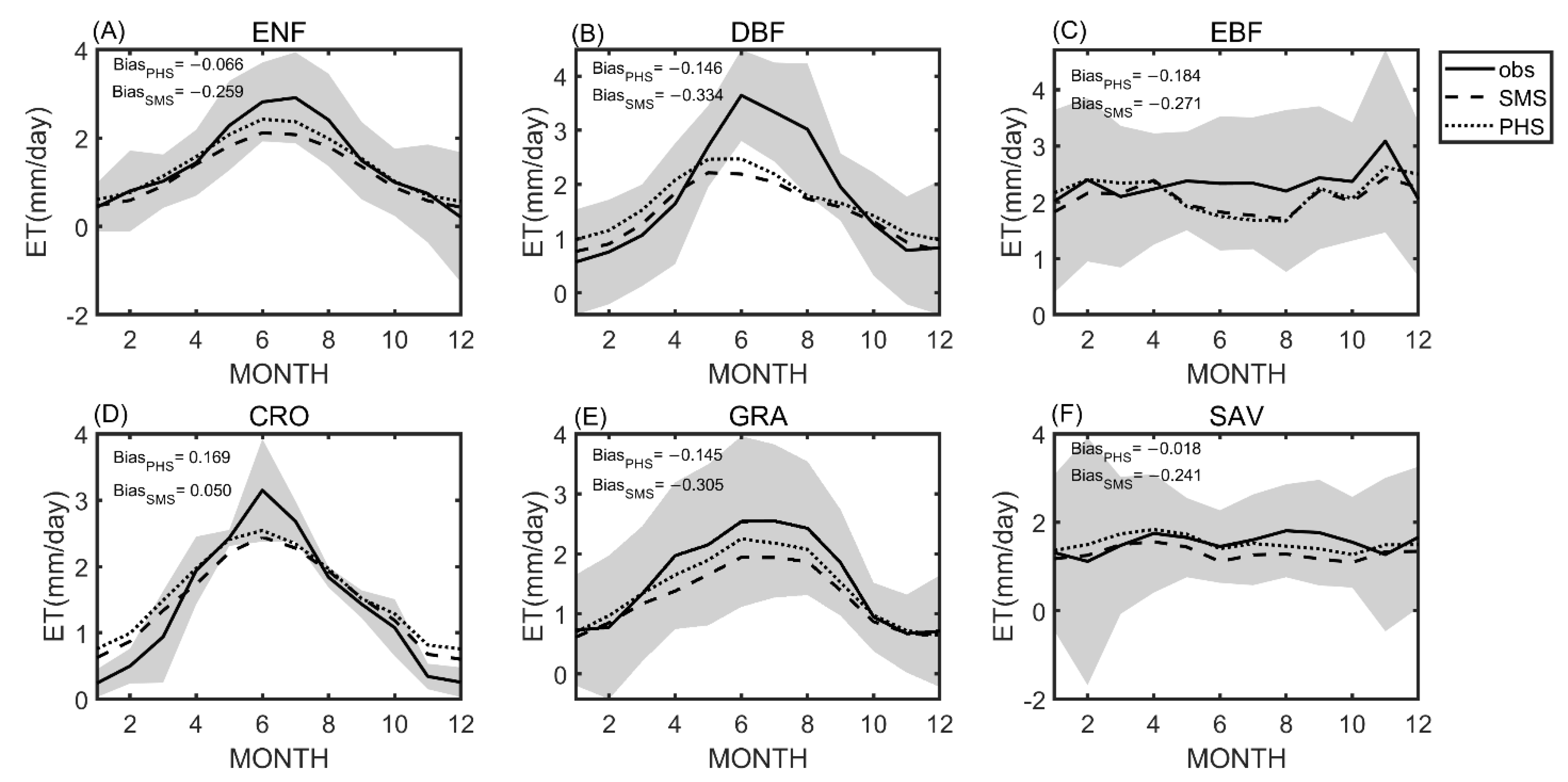
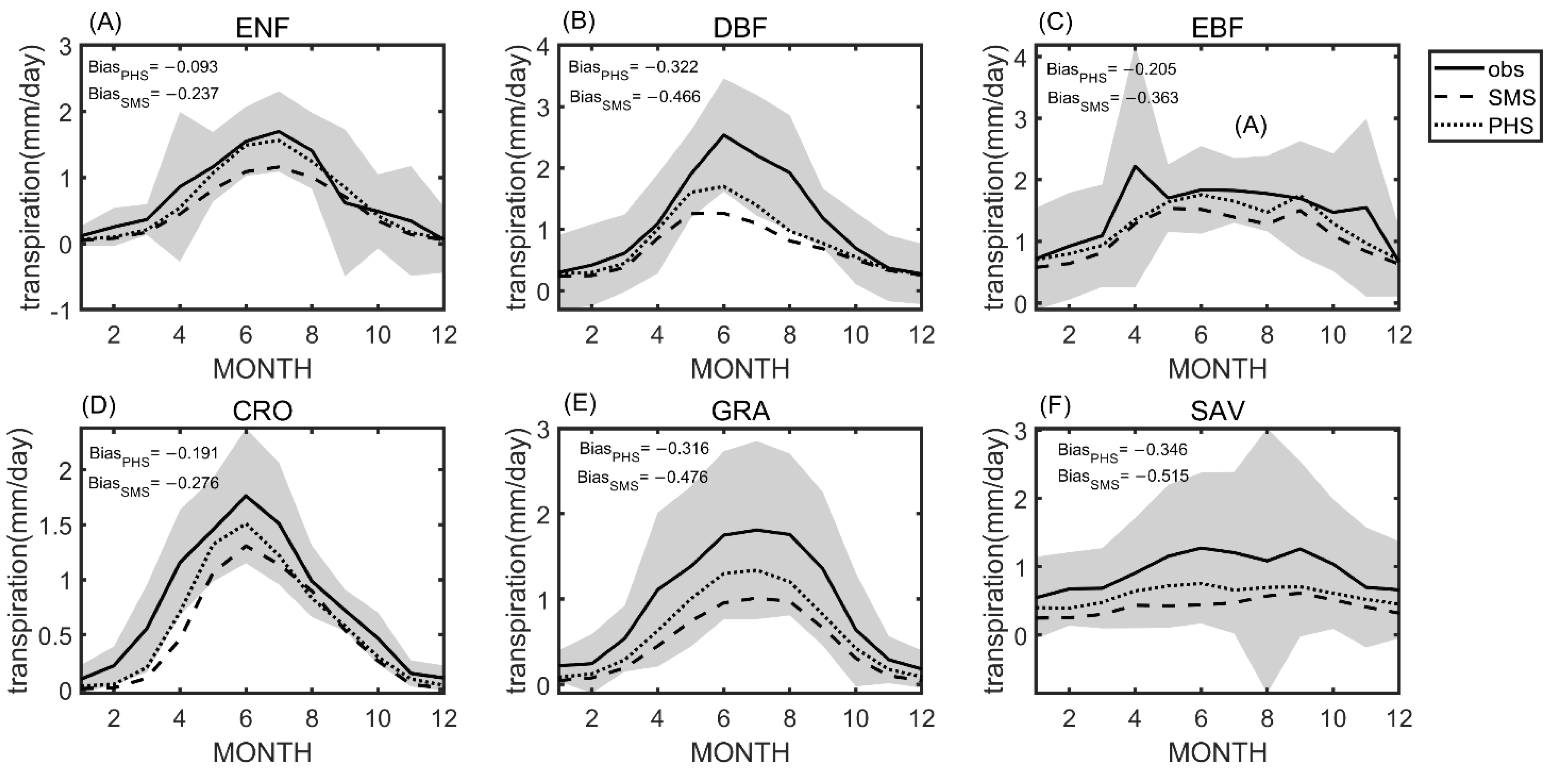
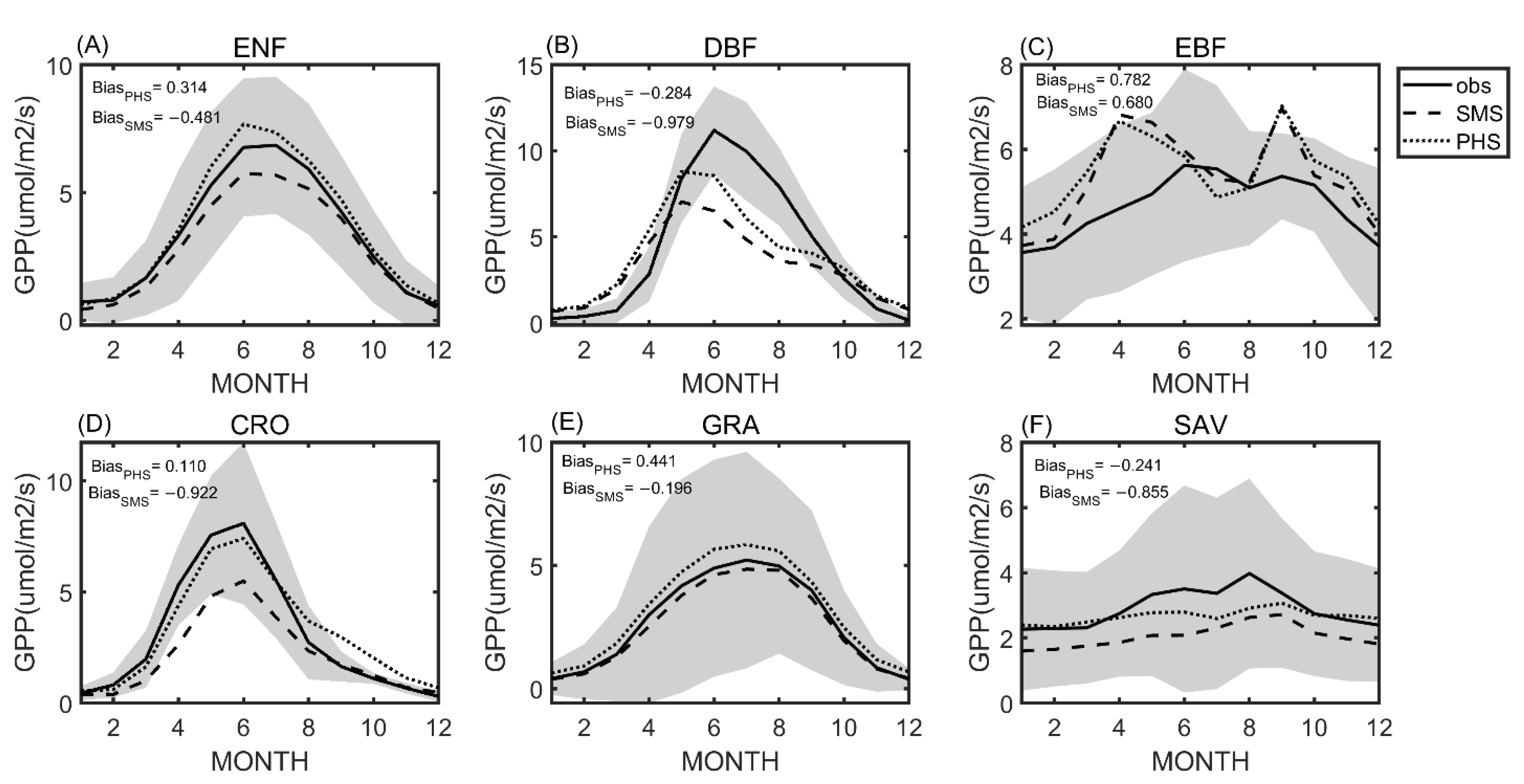
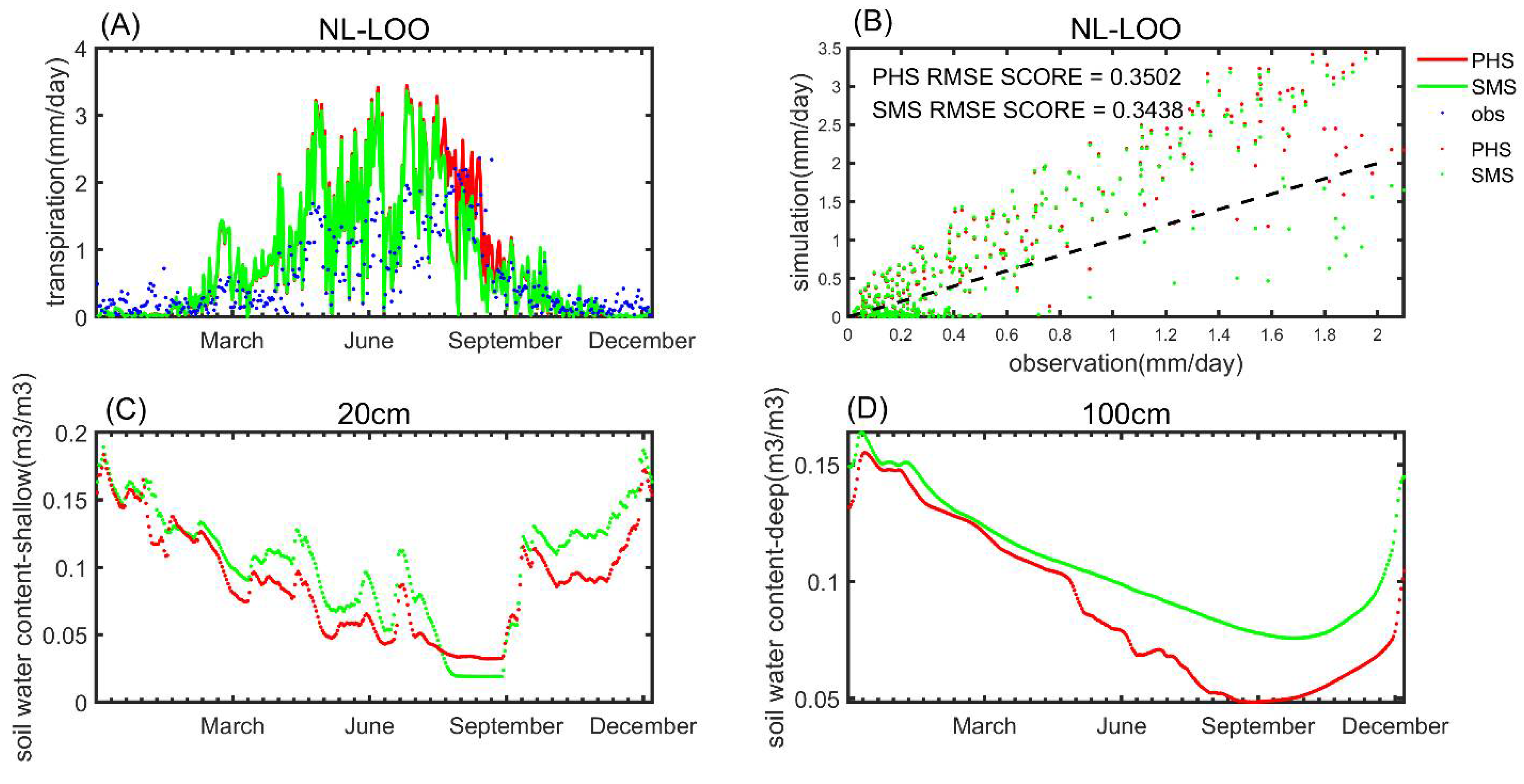
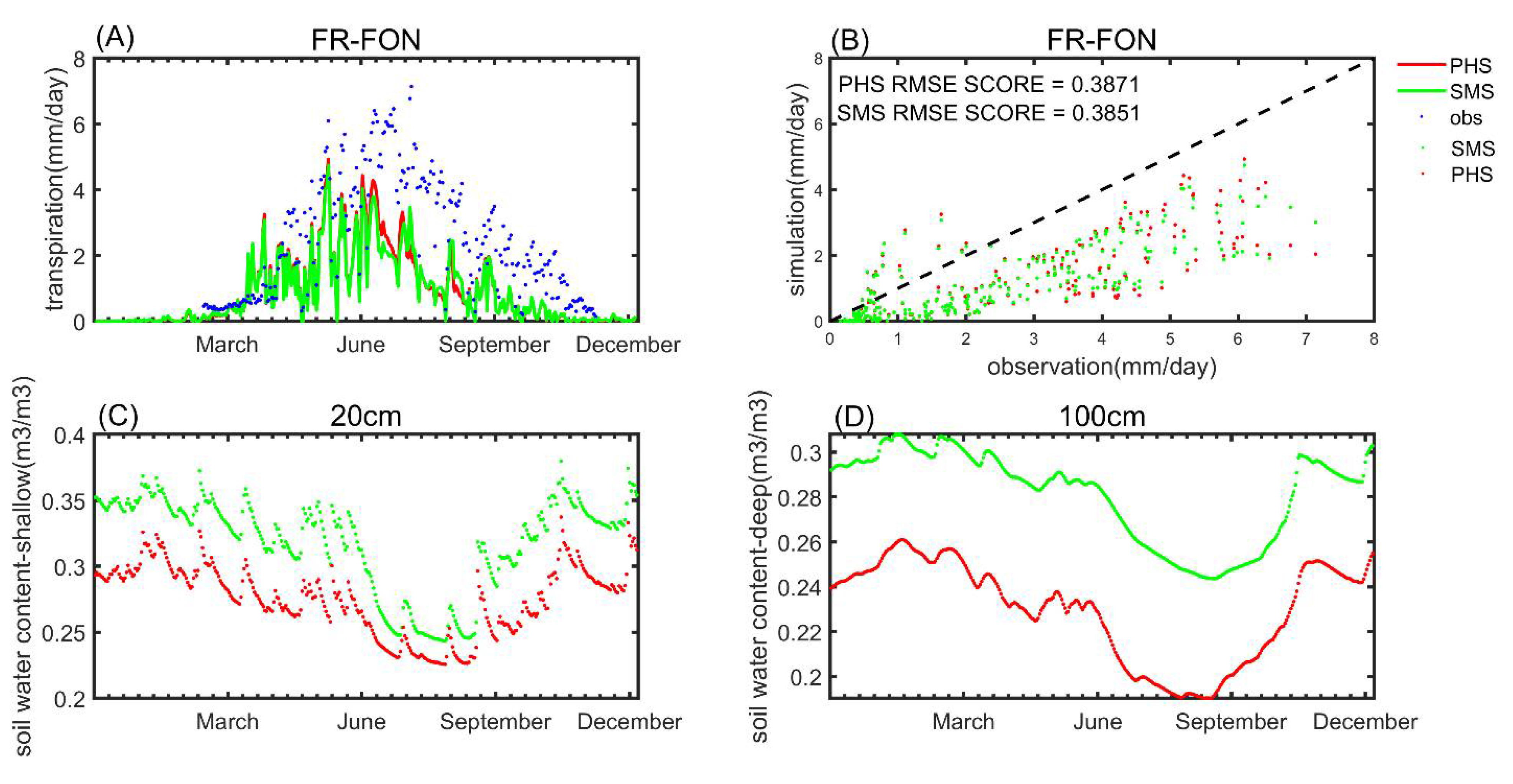
3.1. Seasonal Variation

Figure 2 compared modeled evapotranspiration with observational data. In all plant types, the seasonal variation of evapotranspiration for both PHS and SMS agreed well with the observations. Compared to the default SMS, the new scheme PHS evapotranspiration was significantly improved for the evergreen needle forest (ENF), grassland (GRA), and savanna (SAV), where the bias reduced by 74.5%, 52.5%, and 92.5%, respectively. In deciduous broadleaf forest (DBF) and cropland (CRO), the evapotranspiration only improved for the summer but was overestimated in the winter. The seasonal variation of evapotranspiration was small in evergreen broad forest (EBF) because most EBF sites were tropical. Slight improvements were found only from November to February for EBF.
Figure 3 compared transpiration simulated by PHS and SMS to observational data, separately. For all plant types, both PHS and SMS schemes captured the seasonal variation of transpiration, while the annual mean of transpiration in PHS was closer to the observed annual mean than those in SMS. The improvement in transpiration was much more significant than evapotranspiration. Most improvements occurred in summer when stomata regulation was dominated by soil water stress. For ENF, the transpiration in PHS was highly consistent with the observation, whereas for DBF, CRO, GRA, and SAV, the transpiration from the PHS scenario was slightly underestimated with significant improvement during the summer season. For EBF, there was no significant difference between PHS and SMS. Simultaneously, the climatological mean in the transpiration simulated by PHS fell inside the variation range of the observation, while those simulated by SMS fell outside the variation range for DBF in the summer and CRO in the spring.
Figure 4 compared gross primary productivity (GPP) simulated by PHS and SMS with observational data, separately. PHS for ENF, DBF, CRO, and SAV were less biased in GPP than those in SMS. In ENF, DBF, and CRO, GPP in PHS was improved in summer, whereas GPP in the SAV sites was improved in all seasons. In EBF, GPP in PHS did not differ much from SMS. In GRA, the GPP changed from slightly underestimated in SMS to slightly overestimated in PHS. Overall, the seasonal variation in GPP by PHS was reliable because the climatology means in PHS generally matched the observations. Since plant carbon and water flux were coupled through stomata behavior, the validation in GPP added credit to the transpiration evaluation.
Figure 5A,B compared the modeled transpiration from both PHS and SMS with SAPFLUXNET dataset at NL-LOO. PHS and SMS both captured the seasonal variation of transpiration. Modeled transpiration was higher than observation in summer, and matched well with observation in winter. The RMSE score of PHS (0.35) was slightly higher than SMS (0.34). The seasonal pattern of soil water content was opposite with transpiration. The soil water content in PHS was lower than SMS at both shallow and deep soil layers (Figure 5C,D). The difference is more significant in the deep soil layer than shallow soil layer with more substantial seasonal variation.
Figure 6A,B compared the modeled transpiration from both PHS and SMS with SAPFLUXNET dataset at FR-FON. Modeled transpiration was significantly lower than the sap flow data in summer. The difference of RMSE between PHS and SMS was small. Both shallow and deep soil water content in PHS were significantly lower than SMS. The difference was much smaller in summer than in winter at surface soil (Figure 6C) but with no significant seasonal variation at deep soil (Figure 6D).
Figure 7 illustrated that the root water uptake changed at different soil depths. Positive values indicate water flow from soil to root, while negative values represented the water flow from root to soil. In all cases, the root water uptake was high in the shallow soil layers due to the rich distribution of roots near the surface. At wet sites, both SMS and PHS modeled higher root water uptake in the shallow layers than the deep layers because the soil water was primarily stored in the upper layers due to precipitation. At dry sites, SMS and PHS modeled a monotonical decrease in root water uptake with soil depth, because of fewer roots in the deep soil. However, PHS root water uptake slightly increased in the deep soil because the deep soil moisture was high. PHS relied on the water potential gradient between soil and root more than SMS in modeling root water uptake. The root water uptake of PHS was higher than that of SMS in deep soil, which was at depths between 1.3 and 3.8 m. The root water uptake of PHS was lower than that of SMS in superficial layers, at depths between 0.1 and 1 m (Figure 7A). Root water uptake in wet sites was much higher than in dry sites. In PHS, a higher fraction of water was taken from the deep soil layer in dry sites than in wet sites, whereas in SMS we found no significant differences in the proportion between deep and shallow soil water uptake (Figure 7A).
Seasonal differences (Figure 7B) in root water uptake were much more significant than the site differences (Figure 7A). The root water uptake in the mid and deep soil was much higher in dry seasons than in rainy seasons (Figure 7B). However, the seasonal differences were much weaker in SMS. There were no significant differences in the root water uptake in the shallow layers between PHS and SMS. Therefore, PHS simulated overall higher transpiration than SMS due to the differences in deep root water uptake in dry seasons.
At drier sites (Figure 7C), PHS root water uptake during the rainy season can be even negative at a depth of 0.8–2.0 m, which indicated soil water was transferred to these middle soil layers during the rainy season. Such flow through the root system from shallow to deep can be referred to as the so-called “hydraulic descent”. Similarly, during the dry season in PHS, roots drew most water from deep layers instead of shallow layers. Negative soil water uptake existed at every surface layer. Such flows from deep to shallow were referred to as the “hydraulic lift”. In wetter sites (Figure 7D), although there was no negative root water uptake simulated by PHS, the differences between PHS and SMS were greater in dry seasons than in rainy seasons, especially for deep soil. These patterns indicated that strong HR is simulated by PHS, while the root system played a critical role.
Figure 8 compared the modeled soil water content with observation at 3 FLUXNET sites. PHS and SMS mostly captured the seasonal variation in soil water content, but were just slightly lower than the observation in both shallow and deep soil layer. At US-Var, soil water content in PHS and SMS matched with observation extremely well in shallow soil. Although both PHS and SMS overestimated the deep soil water content in summer, soil water content was slightly improved by PHS. At US-Wkg, the shallow soil water content peaked in summer, when the rainy season came. This seasonal pattern was well captured by both modules, although the deep soil water content was overestimated in winter and underestimated in summer. Overall, both shallow and deep soil water content in PHS and SMS was reasonable at these 3 FLUXNET sites.

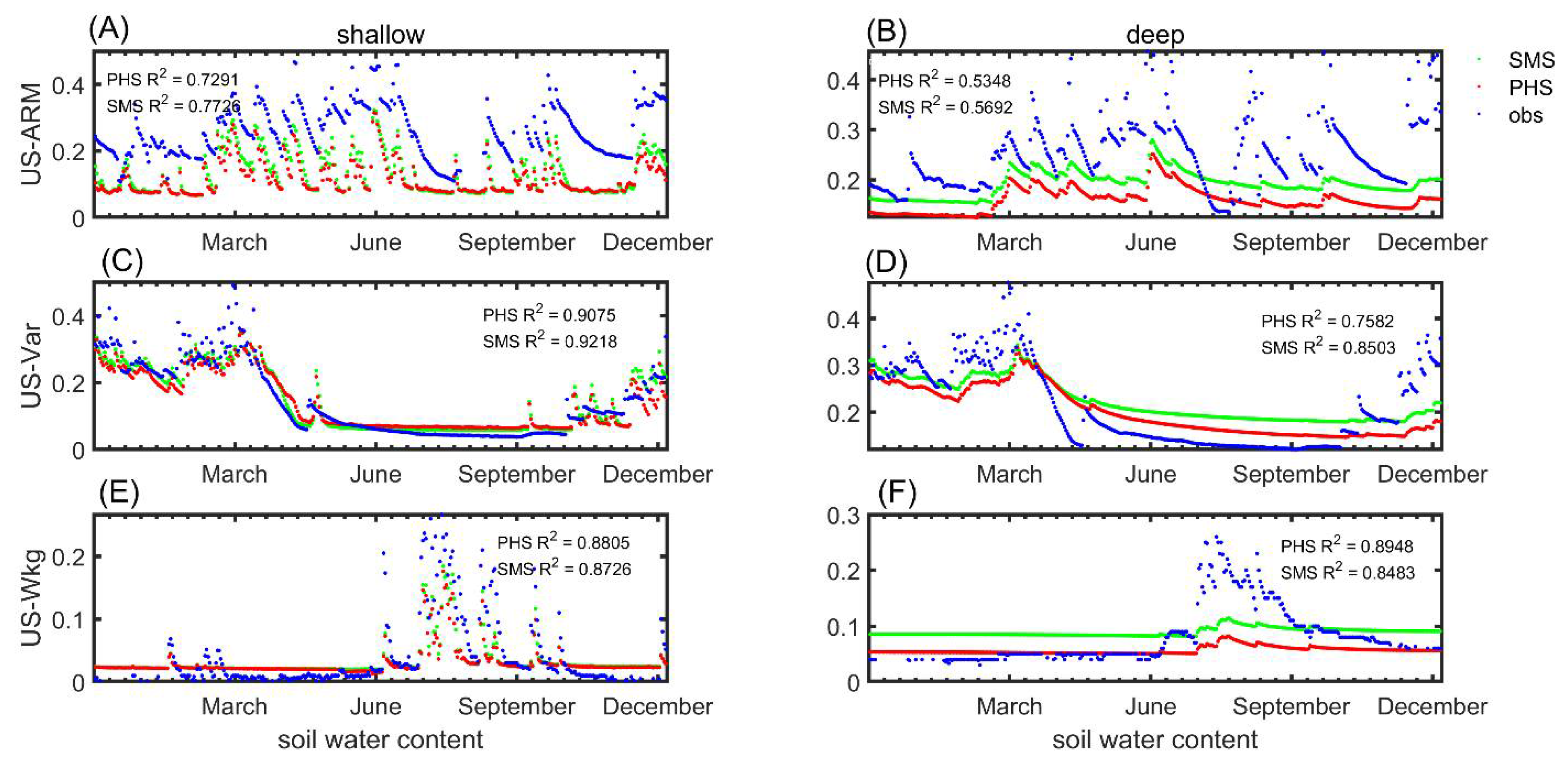
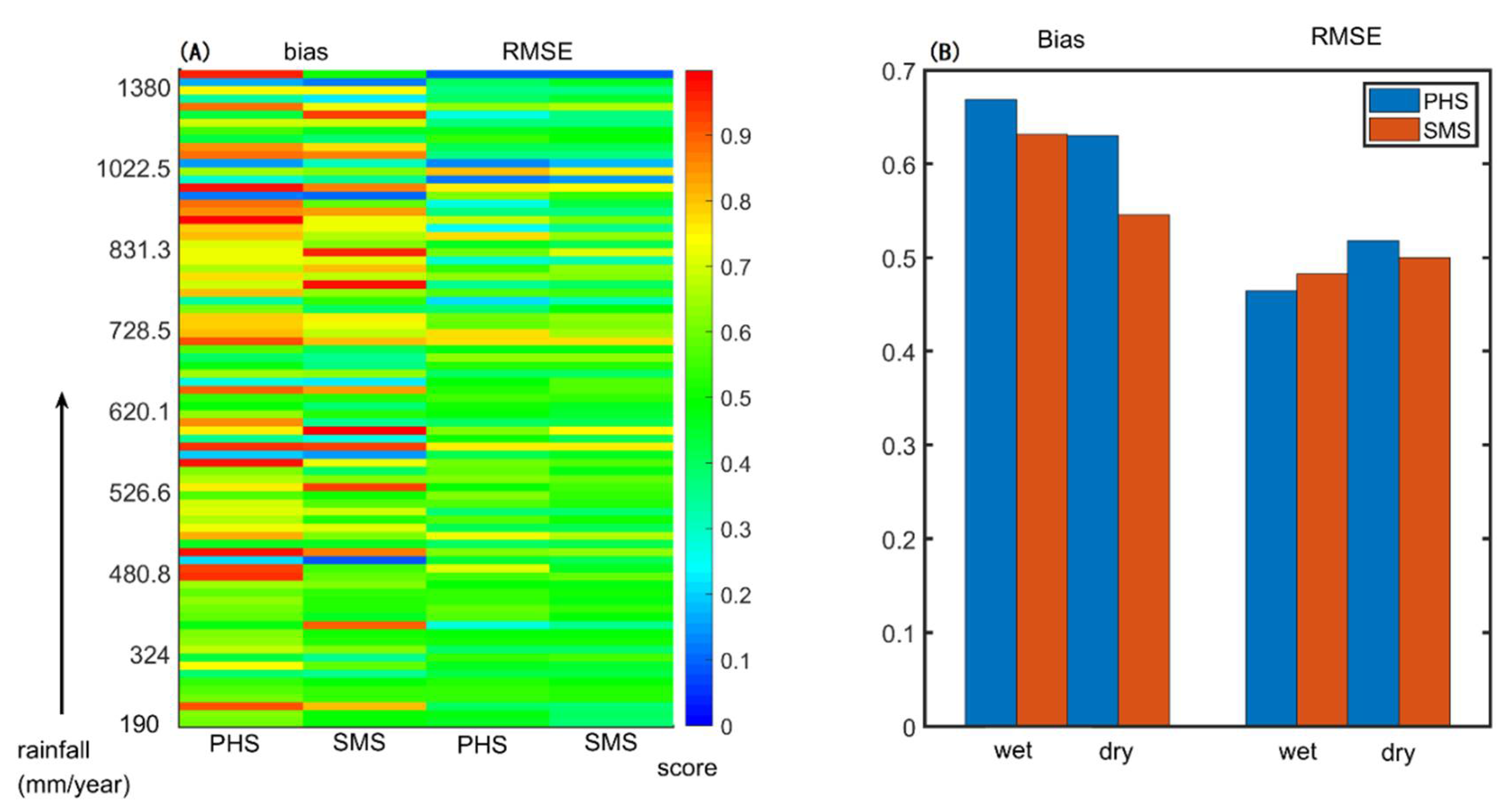
3.2. Benchmarking Analysis

Figure 9 showed that the bias and RMSE score for 81 sites represented by different colors was sorted by the precipitation from wet at the top to dry at the bottom. Wet sites were separated from dry sites by a precipitation threshold, 728 mm, which was the median of all sites. The bias score represented the bias in the temporal average (see details in Section 2.4). The mean bias score was higher for wet sites than the dry sites for both PHS and SMS, which indicated that the CoLM transpiration simulation at dry regions had a considerable potential to improve. At dry sites, the bias score was significantly higher in PHS than SMS. The mean in PHS was 0.63, while the mean in SMS was 0.55. However, at wet sites, the bias score was only slightly higher in PHS than SMS. The mean was 0.66 in PHS and 0.63 in SMS.
The RMSE score represented the bias in the seasonal variability (see details in Section 2.4). The RMSE scores for transpiration at most sites were both between 0.4 and 0.8. The differences between PHS and SMS in RMSE scores were less significant than the bias score. The RMSE score indicated that the PHS modeled seasonal variability in transpiration better than SMS at dry sites, but slightly worse seasonal variability than SMS at wet sites.

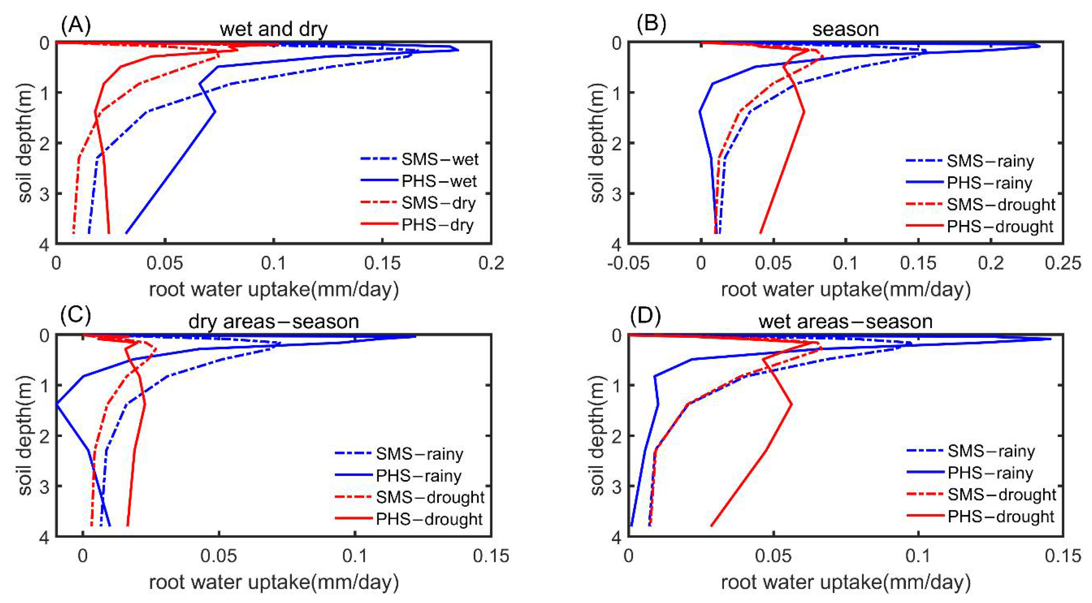
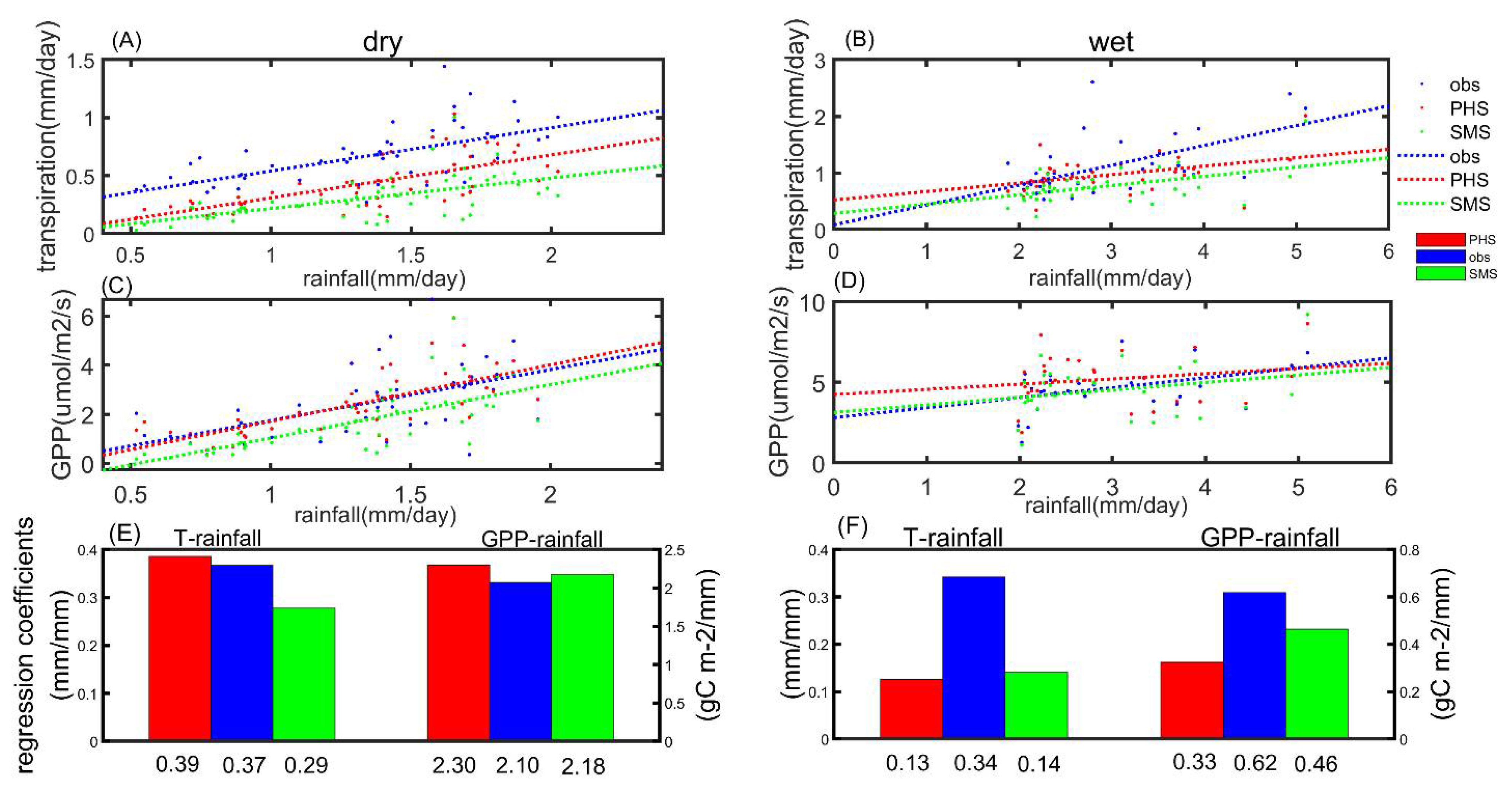
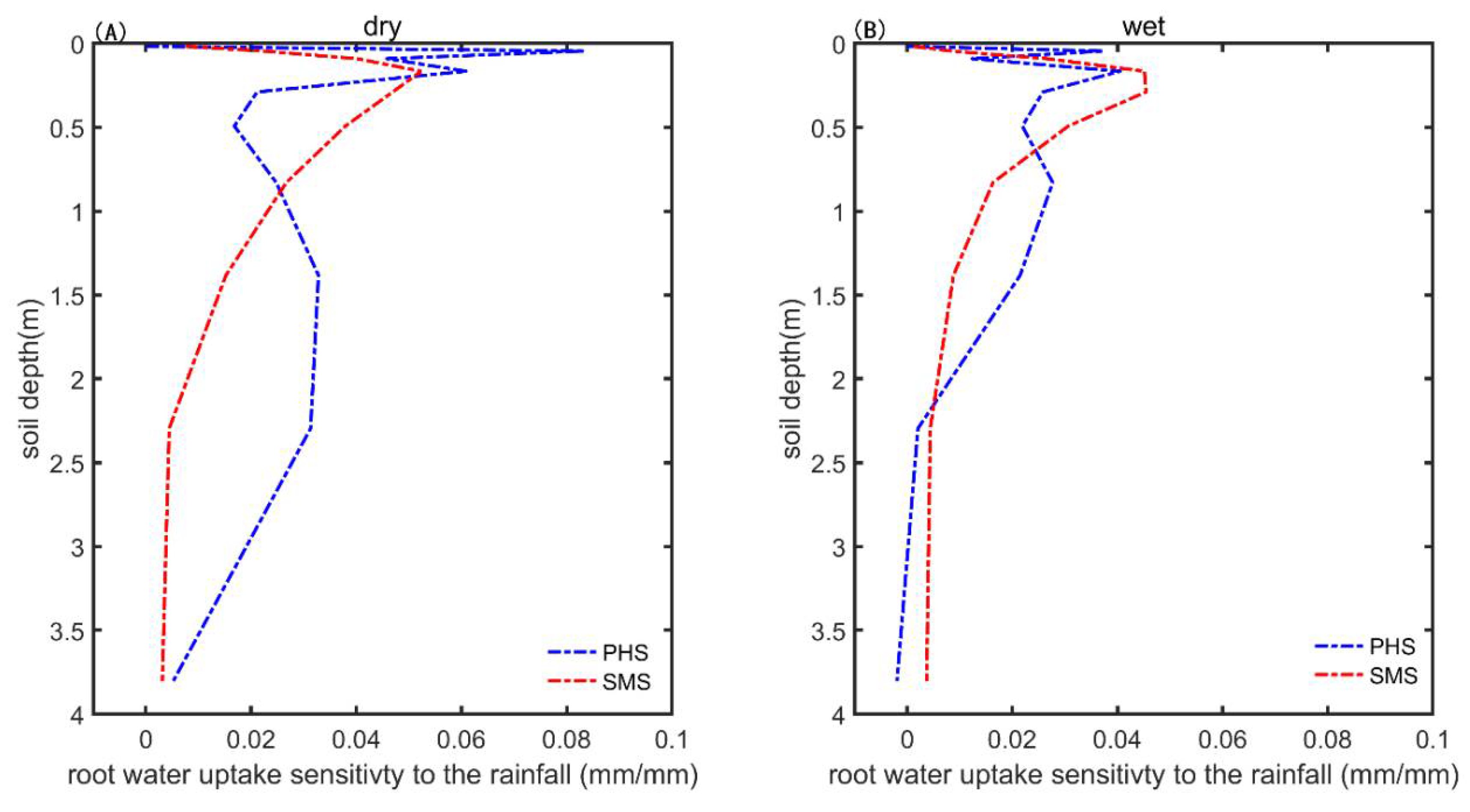
3.3. The Drought Sensitivity

Precipitation was the most dominant meteorological determinant of annual transpiration, which explained over 90% variation in transpiration among various sites (Figure S1). Based on the importance of precipitation, we defined “drought sensitivity” as the slope of the linear regression of transpiration or GPP as a function of precipitation (Figure 10). Among the arid and semi-arid sites, the drought sensitivity for transpiration in PHS (0.39 mm/mm) better matched the observation (0.37 mm/mm) than in SMS (0.28 mm/mm) (Figure 10E). The improvement in drought sensitivity for transpiration may explain the increase in RMSE at arid and semi-arid sites. At humid sites, both PHS and SMS substantially underestimated the drought sensitivity for transpiration, which were 0.13, 0.14, and 0.34 mm/mm for PHS, SMS, and observations, respectively (Figure 10F). The poorly modeled drought sensitivity at wet sites by PHS may account for the lower RMSE in Figure 6.
At arid and semi-arid sites, drought sensitivity for GPP from models well matched that from observations, which were 2.2, 2.1, and 2.0 g·C m−2 mm−1 for PHS, SMS, and observation, respectively (Figure 10E). At humid sites, the drought sensitivity for GPP from the models was significantly lower than those from observation, which were 0.3 g·C m−2 mm−1 and 0.45 g·C m−2 mm−1 for PHS and SMS, and 0.6 for observation, respectively. Due to the coupling between photosynthesis and transpiration through the stomata, underestimating drought sensitivity for GPP may explain the lower drought sensitivity for transpiration.
Plant transpiration was supplied by the uptake of water by roots, which was the major limitation in arid regions. The more pronounced response in PHS transpiration at dry sites compared to SMS was mainly contributed to by deep soil water uptake, which ranged from 0.9 to 3.8 m (Figure 11A). Although the response in shallow root water uptake was slightly weaker in PHS than SMS at depths from 0.2 to 0.9 m, the magnitude was much less than the response in deep water uptake. Overall, HR, which enabled the function of the deep root water uptake, provided a clear response in transpiration to the precipitation. At wet sites, the modeled response to the rainfall is much weaker. Water supply was no longer the limit of the transpiration. Water demand driven by photosynthesis became the primary limit. Due to the underestimates of the photosynthesis response to the precipitation, the PHS root water uptake only positively responded to the precipitation at the depth from 0.7 to 2.2 m, the magnitude of which was very modest.

4. Discussion

4.1. Benchmarking Analysis on Transpiration

Our conclusion that PHS improves transpiration modeling was based on the benchmarking analysis framework. Metrics and benchmarks were two essential components in benchmarking analysis [31]. In our study, we used the bias score to evaluate annual mean transpiration, and we used RMSE score to assess the seasonal variability in transpiration. Both metrics were adopted from the ILAMB project. These benchmarks quantified the model performances and allowed for model comparisons and for comparisons of different regions. For example, the bias score helped us identify that mean transpiration was slightly better modeled by PHS for wet sites than dry sites; the bias scores were 0.66 and 0.63 on average for wet and dry sites, respectively. But the improvements were more significant for dry sites, where the bias score improved from 0.55 by SMS to 0.63 by PHS. Without these metrics, the performance of the models was challenging to infer.
Benchmarks in our study defined the evapotranspiration, transpiration, GPP, and their responses to the precipitation, and aimed to evaluate the performance and attribute the bias of the transpiration simulation. Since direct measurement of transpiration at the stand level was not available, we partitioned the evapotranspiration from FLUXNET into transpiration based on its empirical relationship to LAI. This benchmark was data-derived and contained some degrees of error. Nevertheless, the uncertainties were reduced by using the ensemble mean of different FLUXNET sites distributed worldwide. Moreover, the simulated evapotranspiration agreed well with the direct measurement of latent heat from FLUXNET sites (Figure 2), which enhanced the credibility of the transpiration observation from the evapotranspiration partitioning method. In addition to transpiration and evapotranspiration, we also included GPP as a benchmark. Since transpiration and photosynthesis were usually coupled through the stomata, the inclusion of GPP as one of the benchmarks would help evaluate the stomatal controls on transpiration.
To evaluate mechanistic processes in models, we evaluated modeled responses to precipitation. The response of transpiration or GPP was measured using the slope of the regression of all FLUXNET sites, which was between transpiration and precipitation, or between GPP and precipitation (Figure 10). The slopes represented process-oriented responses. For example, the slopes for GPP in Figure 10C,D indicated how stomata responded to precipitation. The benchmarking on these process-oriented responses was essential, and provided practical and fundamental information about the models.

4.2. Plant Hydraulic Schemes (PHS) Improved the Evapotranspiration Partitioning

Benchmarking analysis on transpiration provided critical information on water cycle modeling and thus improved the modeled interaction between transpiration and the environment. Our results have identified higher modeled transpiration by PHS than SMS. The bias score suggested significant improvements for most FLUXNET sites, especially at the dry sites. The increase in transpiration by PHS has important implications on the evapotranspiration partitioning since most models have underestimated transpiration, including an earlier version of the CLM [10]. Although other factors, such as overestimated soil evaporation, unconstrained vegetation traits, bias in soil hydrology, could contribute to the underestimated evapotranspiration partitioning into transpiration, the absence of the plant hydraulic scheme is at least one of the most important contributing factors. PHS included the HR process that helped root more efficiently absorb deep soil water and, therefore, increased plant transpiration, especially in arid regions.
Recent benchmarking analysis on CLM5 was consistent with our conclusions that the plant hydraulic scheme significantly increased the fraction of transpiration in evapotranspiration in semi-arid regions, especially in the southern hemisphere [14]. The increased evapotranspiration partitioning into transpiration by PHS indicated that plant physiology should have played a more important role in future terrestrial water cycle models. The dominance of the biotic impact on the land–atmosphere water exchange would be more accurately captured by land surface models with PHS.
Overestimates in soil evaporation are possible another reason to explain the underestimate in transpiration fraction in evapotranspiration [10], because soil evaporation competes with transpiration in available soil water content. Overestimated in soil evaporation from the surface soil might further lead to increase in moisture stress and, therefore, further reduce the transpiration fraction. However, PHS plays a vital role in weakening the impact of soil evaporation bias on transpiration fraction. The competition between transpiration and evaporation was significantly reduced in PHS. Soil evaporation primarily uses the water from surface soil. Plant water uptake, which contributes to the transpiration, is mostly from deep soil layers in PHS, while it was initially from shallow soil layers in SMS (Figure 7). Meanwhile, HR in PHS also supplements surface soil water from deep soil layers. Therefore, transpiration and soil evaporation are able to use soil water more efficient in PHS, which enhances the transpiration fraction as well.

4.3. Hydraulic Redistribution (HR) Implementation and the Implication

HR is one of the major processes developed in CoLM PHS. HR, as a widespread phenomenon, has been well documented [32,33]. In recent decades, HR models have successfully simulated “hydraulic lift” in the dry season and “hydraulic decent” in the wet season. The non-negligible impact of HR on climate change modeling has been implied. For example, HR indirectly influences the carbon cycle. More frequent wildfires might be a vital climate change consequence in the future carbon cycle. HR-lifted water from deep soil moisturizes the soil surface and suppresses fire [34]. HR also indirectly impacts the nitrogen cycle. When HR strongly modulates N mineralization, immobilization, and plant N uptake in the dry season, soil nitrogen decomposition and soil nitrate concentration will be significantly decreased. N2O emission is thus reduced [35]. Moreover, HR affects the land–atmosphere water exchange and further feedbacks on the climate. However, the modeled HR magnitude is usually higher than those from the empirical literature. The empirical literature proposed that the HR magnitude ranged from 0.04 to 1.3 mm H2O d−1, whereas the modeled HR magnitude ranged from 0.1 to 3.23 mm H2O d−1 [36]. The lack of data constraints is a major issue in the current development of HR models.
On the one hand, the absence of water flow and water potential measurements in the root system prevents simulations from being more accurate. On the other hand, the unrealistic or simplified HR model structures prevent models from representing the observed counterpart. Regarding the second issue, the more realistic model structure in CoLM PHS might open up a new opportunity for the data constraint on the HR modeling. The PHS in this paper combined the CLM5 PHS model and the HR model by Amenu and Kumar [37]. The root water potential in the new PHS scheme is vertically resolved. Incorporating the vertically resolved water potential into models will allow better data constraints on both root water flow and root water potential. When more individual measurements are available, HR modeling could be improved significantly.
To further improve HR modeling in land surface models, the optimization of soil moisture prediction will provide a more accurate water supply environment for root water uptake modeling. The implementation of HR we introduced was a complicated but more realistic representation of water movement between the soil and roots. Compared to SMS, the deep soil water uptake simulated by PHS with HR was much more sensitive to changes in precipitation (Figure 11). The high quality of the deep soil moisture modeling offers a solid foundation for further improvement in HR modeling. Deep soil moisture is strongly related to the soil water table. Most previous land surface models simulate the water table diagnostically, based on either pressure head profile or a parameterization scheme [38,39]. A numerical framework, which explicitly tracks the soil water table, has opened a novel avenue for soil hydrology modeling [39] and, therefore, improved the quality of the deep soil moisture modeling. Also, the representation of soil hydrology process, soil hydraulic parameters and soil thermal parameters introduce uncertainties in soil moisture prediction [39,40,41,42,43,44]. Soil hydraulic and thermal parameters in land surface models are constrained by soil property datasets and the pedotransfer function (PTF). To minimize the individual bias, Dai et al. [45] used ensemble PTFs to develop global high-resolution and high-quality data for soil hydraulic and thermal parameters. The development in soil hydrology model structure and parameterization and the increasing soil property dataset will reduce the uncertainties in soil moisture prediction and thus improve HR modeling in the future.

4.4. PHS Improved the Transpiration Modeling in Arid or Semi-Arid Regions

Our results suggested that the new plant hydraulic scheme will result in higher transpiration and photosynthesis during dry seasons or in arid regions due to the hydraulic redistribution. Our findings offer an important insight for future climate change modeling. Extreme events, such as drought, are likely to be more frequent in the future [46,47,48,49]. Simulations by coupled climate-carbon-cycle models indicate that an Amazon rainforest dieback could cause more than 100 GtC vegetation carbon loss due to a future drying climate [50,51]. The great vulnerability of the tropical rainforest has been a broad concern [52]. However, stronger transpiration and photosynthesis in arid sites stimulated by PHS suggested that the vegetation should be more tolerant to drought than traditional models using the SMS scheme have suggested. Plants were able to utilize more deep soil water and, therefore, experienced less water stress in our PHS simulations. Thus, PHS simulations suggest that rainforest dieback will be less likely due to the higher water use efficiency.
The improvement in the RMSE (Figure 9) and the drought sensitivity for transpiration (Figure 10A,E) indicated that PHS better simulated plant responses to precipitation. PHS increased the drought sensitivity for transpiration by 33% compared to SMS (Figure 7E) and better matched the observations. The increased drought sensitivity was mainly contributed to by deep soil water uptake (Figure 11A). The deep soil water content depends more on the long-term soil water budget than surface soil. It means annual rainfall is more critical for the deep soil water content than the surface soil, where soil evaporation takes control. Since SMS water uptake is mainly from surface water content, PHS is more sensitive to the annual rainfall than SMS. However, such improvement was only found at dry sites. For humid sites, the RMSE for transpiration was lower for PHS than SMS (Figure 9B). The drought sensitivity for both transpiration and GPP poorly matched the observation (Figure 10F). Both transpiration and GPP were less sensitive than observations. The GPP may be attributed to the insensitivity of transpiration at wet sites (Figure 10D,F), because photosynthesis and transpiration are strongly coupled through stomata. To improve the drought sensitivity for transpiration, we need to understand how GPP responds to precipitation in the models. In current land surface models, the responses to precipitation for GPP were controlled by (1) parameterizations in water stress, (2) stomatal response to VPD, and (3) soil hydrology processes. The improvement in the above processes is essential for future plant hydraulic model development.

4.5. Uncertainties Sources

The LAI derived from MODIS datasets may introduce some additional uncertainties. Due to lack of field observation, it is unable to validate and correct that from the satellite-observed LAI. Although MODIS LAI products have been used in various studies, it is well known that the magnitudes and temporal variations of satellite-derived LAI are somewhat different from those of the field measurements [2]. Meanwhile, we utilized LAI based on empirical regression to obtain observational transpiration. However, there is not a distinction between overstory and understory vegetation in the LAI dataset. In our model, the transpiration of understory was ignored, even though some studies have pointed out that the understory vegetation may contribute 10% to 50% of the evapotranspiration at a stand, and this contribution was related to LAI [53,54]. It is essential to consider the understory impact in model development. Moreover, the data of Wei et al. [2] employed in the development of the regression equations showed a wide variation in transpiration fraction, due to various measurement methods (such as isotopic and non-isotopic) involved. It is well known that different methods showed significant discrepancies among different methods. The inherent errors in FLUXNET and SAPFLUXNET products may also not be negligible. For example, it was found that the energy imbalance problem exists in most sites in the FLUXNET dataset, and scaling single point of sap flow to ecosystem level includes great uncertainties.

5. Conclusions

Here, we evaluated modeled transpiration using CoLM PHS and SMS against FLUXNET data, in which transpiration was separated from evapotranspiration based on an empirical relationship to LAI. The bias score was significantly higher for PHS than SMS at dry sites, which suggested that the improvement of PHS was most significant in dry regions. Generally, the improvement can be interpreted by an increase in transpiration.
Specifically, the increase in transpiration includes two major implications. First, the increase in transpiration results in a better estimate in evapotranspiration partitioning by land surface models. PHS, including the HR scheme, enhances deep-water use. Thus, plants play a more important role in land–atmosphere water exchange. Second, the increase in transpiration, especially in dry regions, indicated that plants in land surface models should have been more tolerant to drought than in previous simulations. The deep-water use relieved plant water stress, and maintained photosynthesis by allowing the stomata to remain open. The plant mortality under more frequent drought in the future should be lower than previously predicted. Future developments in land surface models need to incorporate PHS to improve water cycle modeling, especially in dry regions.
Our benchmarking analysis also identified issues in PHS. The sensitivity of transpiration to the precipitation in wet sites was much lower than the observations. The insensitivity of transpiration can be explained by the underestimate of the sensitivity of GPP, if we assume that photosynthesis covaries with plant water demand by sharing the same mass exchange pathway, the stomata. To better simulate the emergent relationship between transpiration and precipitation, further developments in land surface models may consider improving the parameterization of the plant water stress, soil hydrology processes, or estimates in canopy VPD.

Supplementary Materials

The following are available online at https://www.mdpi.com/article/10.3390/f12060722/s1, Figure S1: The variance explained of rainfall, VPD and radiation to transpiration, respectively. Table S1: FLUXNET site descriptions (Lat and Lon represent latitude and longitude, LAI is annual averaged leaf area index obtained from MODIS datasets, T is mean temperature, P is precipitation, Years is the period with observation, Land cover types are defined by USGS classification.).

Author Contributions

Conceptualization, H.L., X.L. and Z.W.; methodology, X.L. and Z.W.; investigation, H.L.; writing—original draft preparation, H.L.; writing—review and editing, X.L., Z.W., S.Z. (Siguang Zhu), N.W., S.Z. (Shupeng Zhang), H.Y., W.S., S.L., S.Z. (Shulei Zhang), J.H. and Y.D.; visualization, H.L. All authors have read and agreed to the published version of the manuscript.

Funding

This research was funded by the National Key Research and Development Program of China under grants 2017YFA0604300 and 2016YFB0200801, and the Natural Science Foundation of China under grants 41575072, 41730962, 41905075, 42075158 and U1811464.

Data Availability Statement

The data presented in this study are available on request from the corresponding author.

Conflicts of Interest

The authors declare no conflict of interest.

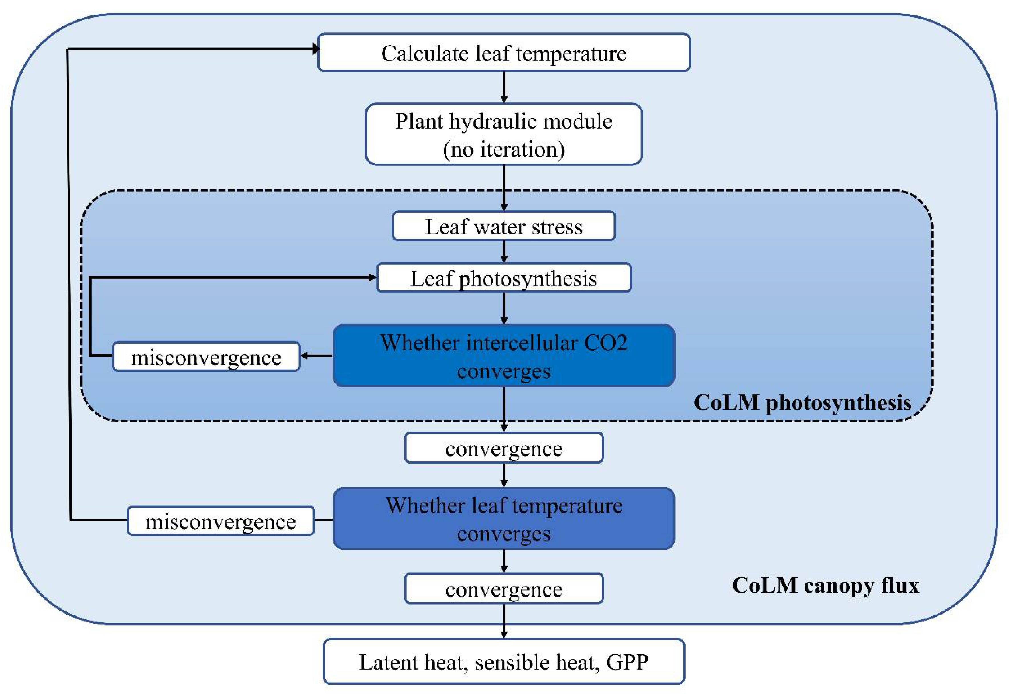
Appendix A. Processes and Parameterizations in the Plant Hydraulic Module

Vegetation water potential is the most fundamental variable for those key processes in PHS. The vegetation water potentials are solved at four aboveground vegetation nodes, and n belowground root nodes. The four aboveground vegetation nodes are sunlit leaf, shaded leaf, stem, and root at the soil surface. By assuming the root system to be a big single root, belowground root nodes represent roots located at different soil depths.
The solution of vegetation water potential depends on stomata conductance and environmental conditions such as atmosphere vapor pressure and soil water matrix potential. The water potential ( Ψ s u n l e a f ,   Ψ s h a l e a f ,   Ψ s t e m , Ψ r o o t , 0 ) at the four aboveground nodes and water flows between them follow the Darcy’s law:
q s u n s t e m = k s u n s t e m ( Ψ s u n l e a f Ψ s t e m )
q s h a s t e m = k s h a s t e m ( Ψ s h a l e a f Ψ s t e m )
q s t e m r o o t = k s t e m r o o t ( Ψ s t e m Ψ r o o t , 0 )
k s u n s t e m , k s h a s t e m and k s t e m r o o t represent hydraulic conductance from stem to sun leaf, stem to shade leaf, and root to stem, respectively. Hydraulic conductance loses with the decline of the water potential. The surface root water potential Ψ r o o t , 0 is solved by coupling Amenu and Kumar’s HR model [19]. The inputs of the HR model include the soil water potential Ψ s o i l , i at each soil layer and the total root water uptake q r o o t , 0 :
Ψ r o o t , 0 = R ( Ψ s o i l , i , q r o o t , 0 )
q s u n s t e m , q s h a s t e m , q s t e m r o o t represents the water flow from stem to sun leaf, from stem to shade leaf, and from root to stem, respectively. The water flow at each node is water conserved due to the assumption that no water is stored in plant organics:
E s u n = q s u n s t e m
E s h a = q s h a s t e m
q s u n s t e m + q s h a s t e m = q s t e m r o o t
q s t e m r o o t = q r o o t , 0
E s u n and E s h a denote transpiration rate of sunlit leaves and shaded leaves. They are products of non-stress transpiration ( E s u n , m a x ,   E s h a , m a x ) and transpiration attenuation function. The non-stress transpiration is simulated by PHS without water stress ( β s u n = 1 ; β s h a = 1 ) . Transpiration attenuation function represents the stomata response to the water stress, which is empirically related to leaf water potential according to a previous experimental study [25]. The attenuation function of transpiration rate varying with leaf water potential ( Ψ s u n l e a f ,   Ψ s h a l e a f ) was introduced into the CoLM plant hydraulic model [14]:
E s u n = E s u n , m a x × 2 ( Ψ s u n l e a f p 50 ) c k
E s h a = E s h a , m a x × 2 ( Ψ s h a l e a f p 50 ) c k
Plant embolization causing serious water transmission capacity loss has also been incorporated. The vulnerability curve [55,56,57,58,59] of the hydraulic conductance, k i j declines with water potential:
k i j = k m a x × 2 ( Ψ j p 50 ) c k
where k m a x is the maximum hydraulic conductance (s−1), i represents the destination node of the flow, and j represents the source node of the flow. Ψ j is the water potential of the source node j (Pa), and p50 is the water potential when the hydraulic conductance is lost by 50% (Pa), and ck is the shape parameter of the fragility curve.
HR in CoLM PHS adopts Amenu and Kumar’s HR model [19]. The hydraulic conductivity in the root system contains axial hydraulic conductivity and radial hydraulic conductivity. The axial hydraulic conductivity is expressed by Darcy’s law:
k a x , i ( Ψ r , i Ψ r , i + 1 ) = q a x , i
where k a x , i is the axial hydraulic conductivity from the root node at (i + 1) th layer to the ith layer, q a x , i is the water flow in ith layer, Ψ r , i is the water potential of the root node at the ith layer. i is from 1 to n − 1, and n represents the total number of soil layers.
Radial hydraulic conduction equation:
k r a d , i ( Ψ s o i l , i Ψ r , i ) = q r a d , i
where k r a d , i is the radial hydraulic conductivity, q r a d , i is the water flow from soil to root, Ψ s o i l , i is the soil water potential at the ith layer. The water balance equation is:
q a x , i + q r a d , i = q a x , i 1
where i is from 2 to n. Thus, Equation (A14) represents n − 1 equations. In addition, from the water balance equation at the surface layer, we can obtain:
q a x , 1 + q r a d , 1 = q r o o t , 0
By combining Equations (A12) and (A13) into (A14) and (A15), we obtain n sets of linear equations about Ψ r , i . These equations describe water flows in the root system, and represent the hydraulic redistribution process as a natural consequence. To solve these equations, Equation (A4) can be explicitly formulated.
The plant water stress is described by water stress factors ( β ) , which constrains the water response in photosynthesis and transpiration. In SMS, the soil water potential ( Ψ i ) determines the water stress factor (β), which is normalized by minimum water potential ( Ψ m i n ) and saturated water potential ( Ψ s a t ):
β = i = 1 n f r o o t i β i
β i = Ψ m a x Ψ i Ψ m a x Ψ s a t
While in PHS, the water stress is supposed to function through stomata closure:
β s u n = g s , s u n g s , s u n , m a x
β s h a = g s , s h a g s , s h a , m a x
where g s , s u n and g s , s h a respectively represent the actual stomatal conductance of the sunny and shaded leaves, and g s , s u n , m a x and g s , s h a , m a x , respectively, represent the maximum stomatal conductance on the sunny and shaded leaves. The solution of water stress requires coupling of the surface canopy turbulence parameterization scheme, Farquhar photosynthesis model, and Ball–Berry stomatal model. The Ball–Berry stomatal model describes the relationship between stomata conductance ( g s ) and photosynthetic rate ( f p h o t o ) , which is modulated by the water stress factors on both sunlit leaf and shaded leaf:
g s u n = g ( f p h o t o ( β s u n ) )
g s h a = g ( f p h o t o ( β s h a ) )
The maximum or actual transpiration rate is calculated from maximum or actual stomata conductance by a latent heat parameterization method similar to CLM5 (See CLM5 technique note, Equation (5.114) [60]:
E s u n , m a x = E ( g s , s u n , m a x )
E s h a , m a x = E ( g s , s h a , m a x )
E s u n = E ( g s , s u n )
E s h a = E ( g s , s h a )
By combining the above equations, the unknowns including plant water potentials Ψ s u n l e a f ,   Ψ s h a l e a f ,   Ψ s t e m , Ψ r o o t , 0 ,   Ψ r , i , and water flows between vegetation nodes, q s u n s t e m ,   q s h a s t e m ,   q s t e m r o o t , q r o o t , 0 , q a x , i , q r a d , i ,   E s u n , m a x , E s h a , m a x ,   E s u n ,   E s h a and stomata conductance g s , s u n , m a x ,   g s , s h a , m a x ,   g s , s u n ,   g s , s h a can be solved numerically.

Appendix B. PHS Solution

To solve plant water potential, water stress, stomatal conductance, and leaf transpiration rate, plant hydraulic module need to be coupled with the photosynthetic stomatal model and surface canopy parameterization scheme. The aim is to solve 18 unknowns from 18 equations in Appendix A. The 18 unknowns include four plant aboveground water potentials ( Ψ s u n l e a f ,   Ψ s h a l e a f ,   Ψ s t e m ,   Ψ r o o t , 0 ), eight water transmission rates ( q s u n s t e m , q s h a s t e m , q s t e m r o o t , q r o o t , 0 , E s u n , m a x , E s h a , m a x ,   E s u n ,   E s h a ), four stomatal conductances ( E s u n , m a x , E s h a , m a x , E s u n ,   E s h a ), and two water stresses ( β s u n , β s h a ). However, since implicit equations were involved, we employed numerical solution to solve the problem. Figure A1 showed the flow chart of PHS solution, and Table A1 showed the parameters in PHS. The numerical solution includes:
(1)
calculate the leaf temperature based on canopy model ( T l , s u m , T l , s h a ).
(2)
calculate the maximum stomatal conductance based on photosynthetic stomata model ( g s , s u n , m a x and g s , s u n , m a x ).
(3)
calculate the maximum leaf transpiration rate according to the maximum stomatal conductance ( E s u n , m a x and E s u n , m a x ).
(4)
calculate the water stress ( β s u n ,   β s h a ).
(5)
update the water stress in the photosynthetic stomata model, and check whether the intercellular carbon dioxide concentration is converged. If it converges, go to step (6); Otherwise, repeat step (5).
(6)
update the stomata conductance, and check whether the water stress converges. If it converges, go to step (7); otherwise, go back to step (2);
(7)
update the plant water potential and leaf transpiration, and check whether the leaf temperatemperature based on canopy model n the plant hydraulic model are solved. Otherwise, go back to step (1).
Figure A1. The flow chart of the PHS solution.
Forests 12 00722 g0a1
Table A1. The values of important parameters in PHS.
Plant Hydraulic ParameterParameter NameDescriptionLand Surface Cover TypeValuesUnits
P50Water potential at 50% loss of leaf tissue conductanceEvergreen Needleleaf Forest−465,000.0mmH2O
Deciduous Broadleaf Forest−270,000.0
Evergreen Broadleaf Forest−260,000.0
Cropland−340,000.0
Grassland−340,000.0
Savanna−340,000.0
hCanopy topEvergreen Needleleaf Forest17.0m
Deciduous Broadleaf Forest19.3
Evergreen Broadleaf Forest35.0
Cropland0.5
Grassland0.5
Savanna0.5
KmaxMaximum hydraulic conductanceALL2.0 × 10−8s−1
CkShape-fitting parameter for vulnerability curveALL3.95
Stomatal Conductance ParameterParameter nameDescriptionPlant typeValuesUnits
G0Conductance-photosynthesis interceptionC39.0
C44.0
α1Conductance-photosynthesis slope parameterC30.01mol CO2·m−2·s−1
C40.04

References

  1. Good, S.P.; Noone, D.; Bowen, G. Hydrologic connectivity constrains partitioning of global terrestrial water fluxes. Science 2015, 349, 175–177. [Google Scholar] [CrossRef] [PubMed] [Green Version]
  2. Wei, Z.; Yoshimura, K.; Wang, L.; Miralles, D.G.; Jasechko, S.; Lee, X. Revisiting the contribution of transpiration to global terrestrial evapotranspiration. Geophys. Res. Lett. 2017, 44, 2792–2801. [Google Scholar] [CrossRef] [Green Version]
  3. Sutanto, S.J.; Wenninger, J.; Coenders-Gerrits, A.M.J.; Uhlenbrook, S. Partitioning of evaporation into transpiration, soil evaporation and interception: A comparison between isotope measurements and a HYDRUS-1D model. Hydrol. Earth Syst. Sci. 2012, 16, 2605–2616. [Google Scholar] [CrossRef] [Green Version]
  4. Coenders-Gerrits, A.M.J.; Van Der Ent, R.J.; Bogaard, T.A.; Wang-Erlandsson, L.; Hrachowitz, M.; Savenije, H.H.G. Uncertainties in transpiration estimates. Nature 2014, 506, E1–E2. [Google Scholar] [CrossRef] [PubMed]
  5. Jasechko, S.; Sharp, Z.D.; Gibson, J.J.; Birks, S.J.; Yi, Y.; Fawcett, P.J. Terrestrial water fluxes dominated by transpiration. Nature 2013, 496, 347–350. [Google Scholar] [CrossRef] [PubMed]
  6. Maxwell, R.M.; Condon, L.E. Connections between groundwater flow and transpiration partitioning. Science 2016, 353, 377–380. [Google Scholar] [CrossRef] [Green Version]
  7. Miralles, D.G.; Jiménez, C.; Jung, M.; Michel, D.; Ershadi, A.; McCabe, M.F.; Hirschi, M.; Martens, B.; Dolman, A.J.; Fisher, J.B.; et al. The WACMOS-ET project–Part 2: Evaluation of global terrestrial evaporation data sets. Hydrol. Earth Syst. Sci. 2016, 20, 823–842. [Google Scholar] [CrossRef] [Green Version]
  8. Dirmeyer, P.A.; Gao, X.; Zhao, M.; Guo, Z.; Oki, T.; Hanasaki, N. GSWP-2: Multimodel analysis and implications for our perception of the land surface. Bull. Am. Meteorol. Soc. 2006, 87, 1381–1397. [Google Scholar] [CrossRef] [Green Version]
  9. Lawrence, D.M.; Oleson, K.W.; Flanner, M.G.; Thornton, P.E.; Swenson, S.C.; Lawrence, P.J.; Zeng, X.; Yang, Z.-L.; Levis, S.; Sakaguchi, K.; et al. Parameterization improvements and functional and structural advances in Version 4 of the Community Land Model. J. Adv. Model. Earth Syst. 2011, 3, 1–27. [Google Scholar]
  10. Lawrence, D.M.; Thornton, P.E.; Oleson, K.W.; Bonan, G.B. The Partitioning of Evapotranspiration into Transpiration, Soil Evaporation, and Canopy Evaporation in a GCM: Impacts on Land?Atmosphere Interaction. J. Hydrometeorol. 2007, 8, 862–880. [Google Scholar] [CrossRef]
  11. Yoshimura, K.; Miyazaki, S.; Kanae, S.; Oki, T. Iso-MATSIRO, a land surface model that incorporates stable water isotopes. Glob. Planet. Chang. 2006, 51, 90–107. [Google Scholar] [CrossRef]
  12. Wang-Erlandsson, L.; Van Der Ent, R.J.; Gordon, L.J.; Savenije, H.H.G. Contrasting roles of interception and transpiration in the hydrological cycle-Part 1: Temporal characteristics over land. Earth Syst. Dyn. 2014, 5, 441–469. [Google Scholar] [CrossRef] [Green Version]
  13. Oleson, K.W.; Lawrence, D.M.; Bonan, G.B.; Drewniak, B.; Huang, M.; Charles, D.; Levis, S.; Li, F.; Riley, W.J.; Zachary, M.; et al. Technical Description of Version 4.5 of the Community Land Model (CLM); NCAR Technical Note NCAR: Boulder, CO, USA, 2013. [Google Scholar]
  14. Kennedy, D.; Swenson, S.; Oleson, K.W.; Lawrence, D.M.; Fisher, R.; Lola da Costa, A.C.; Gentine, P. Implementing Plant Hydraulics in the Community Land Model, Version 5. J. Adv. Model. Earth Syst. 2019, 11, 485–513. [Google Scholar] [CrossRef]
  15. Klein, T.; Rotenberg, E.; Cohen-Hilaleh, E.; Raz-Yaseef, N.; Tatarinov, F.; Preisler, Y.; Ogée, J.; Cohen, S.; Yakir, D. Quantifying transpirable soil water and its relations to tree water use dynamics in a water-limited pine forest. Ecohydrology 2014, 7, 409–419. [Google Scholar] [CrossRef]
  16. Nadezhdina, N.; David, T.S.; David, J.S.; Ferreira, M.I.; Dohnal, M.; Tesař, M.; Gartner, K.; Leitgeb, E.; Nadezhdin, V.; Cermak, J.; et al. Trees never rest: The multiple facets of hydraulic redistribution. Ecohydrology 2010, 3, 431–444. [Google Scholar] [CrossRef]
  17. Schulze, E.D.; Caldwell, M.M.; Canadell, J.; Mooney, H.A.; Jackson, R.B.; Parson, D.; Scholes, R.; Sala, O.E.; Trimborn, P. Downward flux of water through roots (i.e., inverse hydraulic lift) in dry Kalahari sands. Oecologia 1998, 115, 460–462. [Google Scholar] [CrossRef] [PubMed]
  18. Ryel, R.J.; Caldwell, M.M.; Yoder, C.K.; Or, D.; Leffler, A.J. Hydraulic redistribution in a stand of Artemisia tridentata: Evaluation of benefits to transpiration assessed with a simulation model. Oecologia 2002, 130, 173–184. [Google Scholar] [CrossRef]
  19. Amenu, G.G.; Kumar, P. A model for hydraulic redistribution incorporating coupled soil-root moisture transport. Hydrol. Earth Syst. Sci. 2008, 12, 55–74. [Google Scholar] [CrossRef] [Green Version]
  20. Poyatos, R.; Granda, V.; Flo, V.; Adams, M.A.; Oliveira, R.S. Global transpiration data from sap flow measurements: The SAPFLUXNET database. Earth Syst. Sci. Data Discuss. 2020, 1–57. [Google Scholar] [CrossRef]
  21. Pastorello, G.; Trotta, C.; Canfora, E.; Chu, H.; Christianson, D.; Cheah, Y.-W.; Poindexter, C.; Chen, J.; Elbashandy, A.; Humphrey, M.; et al. The FLUXNET2015 dataset and the ONEFlux processing pipeline for eddy covariance data. Sci. Data 2020, 7, 225. [Google Scholar] [CrossRef]
  22. Bonan, G.B. Land Surface Model (LSM Version 1.0) for Ecological, Hydrological, and Atmospheric Studies: Technical Description and User’s Guide; Technical note; Climate and Global Dynamics Division; National Center for Atmospheric Research: Boulder, CO, USA, 1996. [Google Scholar]
  23. Dai, Y.; Dickinson, R.E.; Wang, Y.-P. A Two-Big-Leaf Model for Canopy Temperature, Photosynthesis, and Stomatal Conductance. J. Clim. 2004, 17, 2281–2299. [Google Scholar] [CrossRef]
  24. Dai, Y.; Zeng, X.; Dickinson, R.E.; Baker, I.; Bonan, G.B.; Bosilovich, M.G.; Denning, A.S.; Dirmeyer, P.A.; Houser, P.R.; Niu, G.; et al. The common land model. Bull. Am. Meteorol. Soc. 2003, 84, 1013–1023. [Google Scholar] [CrossRef] [Green Version]
  25. Klein, T. The variability of stomatal sensitivity to leaf water potential across tree species indicates a continuum between isohydric and anisohydric behaviours. Funct. Ecol. 2014, 28, 1313–1320. [Google Scholar] [CrossRef]
  26. Wilson, K.; Goldstein, A.; Falge, E.; Aubinet, M.; Verma, S. Energy balance closure at FLUXNET sites. Agric. Meteorol. 2002, 113, 223–243. [Google Scholar] [CrossRef] [Green Version]
  27. Zhang, X.; Dai, Y.; Cui, H.; Dickinson, R.E.; Zhu, S.; Wei, N.; Yan, B.; Yuan, H.; Shangguan, W.; Wang, L.; et al. Evaluating common land model energy fluxes using FLUXNET data. Adv. Atmos. Sci. 2017, 34, 1035–1046. [Google Scholar] [CrossRef]
  28. Nelson, J.A.; Pérez-Priego, O.; Zhou, S.; Poyatos, R.; Zhang, Y.; Blanken, P.D.; Gimeno, T.E.; Wohlfahrt, G.; Desai, A.R.; Gioli, B. Ecosystem transpiration and evaporation: Insights from three water flux partitioning methods across FLUXNET sites. Glob. Chang. Biol. 2020, 26, 6916–6930. [Google Scholar] [CrossRef]
  29. Yuan, H.; Dai, Y.; Xiao, Z.; Ji, D.; Shangguan, W. Reprocessing the MODIS Leaf Area Index products for land surface and climate modelling. Remote Sens. Environ. 2011, 115, 1171–1187. [Google Scholar] [CrossRef]
  30. Collier, N.; Hoffman, F.M.; Lawrence, D.M.; Keppel-Aleks, G.; Koven, C.D.; Riley, W.J.; Mu, M.; Randerson, J.T. The International Land Model Benchmarking (ILAMB) System: Design, Theory, and Implementation. J. Adv. Model. Earth Syst. 2018, 10, 2731–2754. [Google Scholar] [CrossRef] [Green Version]
  31. Luo, Y.Q.; Randerson, J.T.; Abramowitz, G.; Bacour, C.; Blyth, E.; Carvalhais, N.; Ciais, P.; Dalmonech, D.; Fisher, J.B.; Fisher, R.; et al. A framework for benchmarking land models. In Biogeosciences; Copernicus Publications: Göttingen, Germany, 2012; Volumn 9, pp. 3857–3874. [Google Scholar]
  32. Caldwell, M.M.; Dawson, T.E.; Richards, J.H. Hydraulic lift: Consequences of water efflux from the roots of plants. Oecologia 1998, 113, 151–161. [Google Scholar] [CrossRef] [PubMed]
  33. Jackson, R.B.; Sperry, J.S.; Dawson, T.E. Root water uptake and transport: Using physiological processes in global predictions. Trends Plant Sci. 2000, 5, 482–488. [Google Scholar] [CrossRef]
  34. Fu, C.; Wang, G.; Bible, K.; Goulden, M.L.; Saleska, S.R.; Scott, R.L.; Cardon, Z.G. Hydraulic redistribution affects modeled carbon cycling via soil microbial activity and suppressed fire. Glob. Chang. Biol. 2018, 24, 3472–3485. [Google Scholar] [CrossRef]
  35. Fu, C.; Lee, X.; Griffis, T.J.; Wang, G.; Wei, Z. Influences of Root Hydraulic Redistribution on N2O Emissions at AmeriFlux Sites. Geophys. Res. Lett. 2018, 45, 5135–5143. [Google Scholar] [CrossRef]
  36. Neumann, R.B.; Cardon, Z.G. The magnitude of hydraulic redistribution by plant roots: A review and synthesis of empirical and modeling studies. New Phytol. 2012, 194, 337–352. [Google Scholar] [CrossRef]
  37. Zhu, S.; Chen, H.; Zhang, X.; Wei, N.; Shangguan, W.; Yuan, H.; Zhang, S.; Wang, L.; Zhou, L.; Dai, Y. Incorporating root hydraulic redistribution and compensatory water uptake in the common land model: Effects on site level and global land modeling. J. Geophys. Res. 2017, 122, 7308–7322. [Google Scholar] [CrossRef]
  38. Lawrence, D.; Fisher, R.; Koven, C.; Oleson, K.; Swenson, S.; Vertenstein, M. CLM5 Documentation; NCAR Technical Note NCAR: Boulder, CO, USA, 2018. [Google Scholar]
  39. Bisht, G.; Riley, W.J.; Hammond, G.E.; Lorenzetti, D.M. Development and evaluation of a variably saturated flow model in the global E3SM Land Model (ELM) version 1.0. Geosci. Model. Dev. 2018, 11, 4085–4102. [Google Scholar] [CrossRef] [Green Version]
  40. Dai, Y.; Wei, N.; Yuan, H.; Zhang, S.; Shangguan, W.; Liu, S.; Lu, X.; Xin, Y. Evaluation of soil thermal conductivity schemes for use in land surface modeling. J. Adv. Modeling Earth Syst. 2019, 11, 3454–3473. [Google Scholar] [CrossRef]
  41. Baroni, G.; Facchi, A.; Gandolfi, C.; Ortuani, B.; Horeschi, D.; Van Dam, J.C. Uncertainty in the determination of soil hydraulic parameters and its influence on the performance of two hydrological models of different complexity. Hydrol. Earth Syst. Sci. Discuss. 2009, 6, 4065–4105. [Google Scholar]
  42. Christiaens, K.; Feyen, J. Analysis of uncertainties associated with different methods to determine soil hydraulic properties and their propagation in the distributed hydrological MIKE SHE model. J. Hydrol. 2001, 246, 63–81. [Google Scholar] [CrossRef]
  43. Freer, J.; Beven, K.; Ambroise, B. Bayesian Estimation of Uncertainty in Runoff Prediction and the Value of Data: An Application of the GLUE Approach. Water Resour. Res. 1996, 32, 2161–2173. [Google Scholar] [CrossRef]
  44. Walker, J.P.; Willgoose, G.R.; Kalma, J.D. In situ measurement of soil moisture: A comparison of techniques. J. Hydrol. 2004, 293, 85–99. [Google Scholar] [CrossRef]
  45. Dai, Y.; Xin, Q.; Wei, N.; Zhang, Y.; Shangguan, W.; Yuan, H.; Zhang, S.; Liu, S.; Lu, X. A global high-resolution data set of soil hydraulic and thermal properties for land surface modeling. J. Adv. Modeling Earth Syst. 2019, 11, 2996–3023. [Google Scholar] [CrossRef] [Green Version]
  46. Cai, W.; Wang, G.; Santoso, A.; Mcphaden, M.J.; Wu, L.; Jin, F.F.; Timmermann, A.; Collins, M.; Vecchi, G.; Lengaigne, M.; et al. Increased frequency of extreme La Niña events under greenhouse warming. Nat. Clim. Chang. 2015, 5, 132–137. [Google Scholar] [CrossRef]
  47. Jiménez-Muñoz, J.C.; Mattar, C.; Barichivich, J.; Santamaría-Artigas, A.; Takahashi, K.; Malhi, Y.; Sobrino, J.A.; Schrier, G. van der Record-breaking warming and extreme drought in the Amazon rainforest during the course of El Niño 2015–2016. Sci. Rep. 2016, 6, 33130. [Google Scholar] [CrossRef] [Green Version]
  48. Spinoni, J.; Vogt, J.V.; Naumann, G.; Barbosa, P.; Dosio, A. Will drought events become more frequent and severe in Europe? Int. J. Clim. 2018, 38, 1718–1736. [Google Scholar] [CrossRef] [Green Version]
  49. Zhang, M.; He, J.; Wang, B.; Wang, S.; Li, S.; Liu, W.; Ma, X. Extreme drought changes in Southwest China from 1960 to 2009. J. Geogr. Sci. 2013, 23, 3–16. [Google Scholar] [CrossRef]
  50. Cox, P.M.; Betts, R.A.; Jones, C.D.; Spall, S.A.; Totterdell, I.J. Acceleration of global warming due to carbon-cycle feedbacks in a coupled climate model. Nature 2000, 408, 184–187. [Google Scholar] [CrossRef]
  51. Cox, P.M.; Betts, R.A.; Collins, M.; Harris, P.P.; Huntingford, C.; Jones, C.D. Amazonian forest dieback under climate-carbon cycle projections for the 21st century. Appl. Clim. 2004, 78, 137–156. [Google Scholar] [CrossRef]
  52. Feeley, K.J.; Rehm, E.M. Amazon’s vulnerability to climate change heightened by deforestation and man-made dispersal barriers. Glob. Chang. Biol. 2012, 18, 3606–3614. [Google Scholar] [CrossRef]
  53. Wilson, K.B.; Hanson, P.J.; Baldocchi, D.D. Factors controlling evaporation and energy partitioning beneath a deciduous forest over an annual cycle. Agric. For. Meteorol. 2000, 102, 83–103. [Google Scholar]
  54. Kelliher, F.M.; Hollinger, D.Y.; Schulze, E.; Vygodskaya, N.N.; Byers, J.N.; Hunt, J.E.; Mcseveny, T.M.; Milukova, I.; Sogatchev, A.; Varlargin, A. Evaporation from an eastern Siberian larch forest. Agric. For. Meteorol. 1997, 85, 135–147. [Google Scholar]
  55. Gentine, P.; Guérin, M.; Uriarte, M.; McDowell, N.G.; Pockman, W.T. An allometry-based model of the survival strategies of hydraulic failure and carbon starvation. Ecohydrology 2016, 9, 529–546. [Google Scholar] [CrossRef]
  56. Neufeld, H.S.; Grantz, D.A.; Meinzer, F.C.; Goldstein, G.; Crisosto, G.M.; Crisosto, C. Genotypic Variability in Vulnerability of Leaf Xylem to Cavitation in Water-Stressed and Well-Irrigated Sugarcane. Plant Physiol. 1992, 100, 1020–1028. [Google Scholar] [CrossRef] [Green Version]
  57. Pammenter, N.W.; Van der Willigen, C. A mathematical and statistical analysis of the curves illustrating vulnerability of xylem to cavitation. Tree Physiol. 1998, 18, 589–593. [Google Scholar] [CrossRef] [PubMed] [Green Version]
  58. Plaut, J.A.; Yepez, E.A.; Hill, J.; Pangle, R.; Sperry, J.S.; Pockman, W.T.; Mcdowell, N.G. Hydraulic limits preceding mortality in a piñon–juniper woodland under experimental drought. Plant Cell Environ. 2012, 35, 1601–1617. [Google Scholar] [CrossRef] [PubMed]
  59. Sperry, J.S.; Tyree, M.T. Mechanism of Water Stress-Induced Xylem Embolism. Plant Physiol. 1988, 88, 581–587. [Google Scholar] [CrossRef] [PubMed] [Green Version]
  60. Lawrence, D.M.; Fisher, R.A.; Koven, C.D.; Oleson, K.W.; Swenson, S.C.; Bonan, G.; Collier, N.; Ghimire, B.; van Kampenhout, L.; Kennedy, D.; et al. The Community Land Model Version 5: Description of New Features, Benchmarking, and Impact of Forcing Uncertainty. J. Adv. Model. Earth Syst. 2019, 11, 4245–4287. [Google Scholar] [CrossRef] [Green Version]
Figure 1. Distribution of FLUXNET sites used in this study. Colors represent the 12 vegetation coverage types.
Forests 12 00722 g001
Figure 2. Seasonal variation in evapotranspiration. The climatologic mean in evapotranspiration is the average over all site-year seasonal variations, which is grouped into six plant types ((A), evergreen needleleaf forest; (B), deciduous broadleaf forest; (C), evergreen broadleaf forest; (D), cropland; (E), grassland; (F), savanna). The shadow is the standard deviation of the observation. The BiasPHS is the annual mean difference in evapotranspiration between observation and plant hydraulic schemes (PHS), and BiasSMS is the annual mean difference in evapotranspiration between observation and soil moisture stress (SMS).
Forests 12 00722 g002
Figure 3. Seasonal variation in transpiration. The climatologic mean in transpiration is the average over all site-year seasonal variations, which is grouped into six plant types ((A), evergreen needleleaf forest; (B), deciduous broadleaf forest; (C), evergreen broadleaf forest; (D), cropland; (E), grassland; (F), savanna). The shadow is the standard deviation of the observation. The BiasPHS is the annual mean difference in the transpiration of the observation and PHS, and the BiasSMS is the annual mean difference in the transpiration between the observation and SMS.
Forests 12 00722 g003
Figure 4. Seasonal variation in gross primary productivity (GPP). The climatologic mean in GPP is the average over all site-year seasonal variations, which is grouped into six plant types ((A), evergreen needleleaf forest; (B), deciduous broadleaf forest; (C), evergreen broadleaf forest; (D), cropland; (E), grassland; (F), savanna), The shadow is the standard deviation of the observation. The BiasPHS is the annual mean difference in GPP between the observation and PHS, and the BiasSMS is the annual mean difference in GPP between observation and PHS.
Forests 12 00722 g004
Figure 5. Transpiration (mm/day) and soil water content (m3/m3) at NL-LOO (the site name) in 2012. (A) seasonal variation in transpiration; (B) comparison between simulated transpiration and SAPFLUX data; (C) soil water content simulated by PHS and SMS at shallow soil layer (20 cm); (D) soil water content simulated by PHS and SMS at deep soil layer (100 cm).
Forests 12 00722 g005
Figure 6. Transpiration (mm/day) and soil water content (m3/m3) at FR-FON (the site name) in 2013. (A) seasonal variation in transpiration; (B) comparison between simulated transpiration and SAPFLUX data; (C) soil water content simulated by PHS and SMS at shallow soil layer (20 cm); (D) soil water content simulated by PHS and SMS at deep soil layer (100 cm).
Forests 12 00722 g006
Figure 7. The root water uptake at different depths (mm/day). The vertical profiles are averaged over (A) wet sites versus dry sites; (B) rainy months versus drought months of all sites; (C) rainy months versus drought months of dry sites; (D) rainy months versus drought months of wet sites. The solid line represents PHS, and the dotted line represents SMS. In (A), the blue lines and red lines represent wet sites and dry sites, respectively, and in (B) they represent rainy seasons and drought seasons, respectively.
Forests 12 00722 g007
Figure 8. Comparison of soil water content (m3/m3) between model and observation. (A) the comparison of soil water content at US-ARM in 2007 for shallow soil layer; (B) the comparison of soil water content at US-ARM in 2007 for deep soil layer; (C) the comparison of soil water content at US-Var in 2006 for shallow soil layer; (D) the comparison of soil water content at US-Var in 2006 for deep soil layer; (E) the comparison of soil water content at US-Wkg in 2006 for shallow soil layer; (F) the comparison of soil water content at US-Wkg in 2006 for deep soil layer.
Forests 12 00722 g008
Figure 9. Benchmark results for transpirations. (A) Bias score and root mean square error (RMSE) of transpiration modeled by PHS and SMS at 81 sites; (B) the score average among sites is grouped by dry sites and wet sites, or by PHS and SMS.
Forests 12 00722 g009
Figure 10. Drought sensitivity of transpiration and GPP. (A,B) are unary regression between T and precipitation. (C,D) are unary regression between GPP and precipitation. (E,F) are regression coefficients. The figures in the right column are the results from the dry sites, and the figures from the left column are the results from the wet sites.
Forests 12 00722 g010
Figure 11. Drought sensitivity of root water uptake (A) depicts the sensitivity of root water uptake in each soil layer to precipitation in dry areas; (B) is the same as (A), but for wet areas. Sensitivity refers to the regression coefficient between root water uptake of each layer and precipitation.
Forests 12 00722 g011
Table 1. Regression fitting coefficient values of six vegetation types.
Plant Cover Typesab
Needle-leaf forests0.480.32
Broad-leaf forests0.640.15
Mixed and forests0.520.26
Shrubs and grasses0.690.28
Crops0.660.18
Wetlands0.650.21
Publisher’s Note: MDPI stays neutral with regard to jurisdictional claims in published maps and institutional affiliations.

