Abstract
Performance-based, service-life design of wood has been the focus of much research in recent decades. Previous works have been synthesized in various factorized design frameworks presented in the form of technical reports. Factorization does not consider the non-linear dependency between decay-influencing effects, such as between detail design and climate variables. The CLICKdesign project is a joint European effort targeting digital, performance-based specification for service-life design (SLD) of wood. This study evaluates the feasibility of using a semi-empirical moisture model (SMM) as a basis for a digital SLD framework. The performance of the SMM is assessed by comparison against a finite element model (FEM). In addition, two different wood decay models (a logistic, LM, and simplified logistic model (SLM)) are compared. While discrepancies between the SMM and FEM were detected particularly at high wood moisture content, the overall performance of the SMM was deemed sufficient for the application. The main source of uncertainty instead stems from the choice of wood decay model. Based on the results, a new method based on pre-calculated time series, empirical equations, and interpolation is proposed for predicting the service life of wood. The method is fast and simple yet able to deal with non-linear effects between weather variables and the design of details. As such, it can easily be implemented as part of a digital design guideline to provide decision support for architects and engineers, with less uncertainty than existing factorized guidelines.
1. Introduction
The durability of wood depends on factors related to the material, such as species, growth conditions, and quality, as well as factors related to the environment, such as local climatic conditions, protection by design, and detailing [1]. The design of wooden commodities has historically relied on adherence to local design traditions which have evolved largely through trial-and-error. Even today, much of the knowledge involved in the design of wooden commodities is fragmented and unavailable to non-wood experts. Eurocode 5 [2] refers to EN 460 [3], which recommends a minimum durability class [4] for each hazard class, where the latter accounts for the moisture exposure at hand. The hazard classes have largely been replaced by use-class definitions according to EN 335 [5]. As stated in EN 335: “A use class is not a performance class and does not give guidance for how long wood and wood-based products will last in service”. Use classes are also defined in broad terms and are not very nuanced. For example, subclass 3.2 includes any type of moisture trap, ranging from permanently damp conditions to rather dry ones.
It is well-known that wood deterioration by decay fungi is related to wood temperature and moisture content. The moisture content in turn depends on weather conditions, design of detailing, wood species, and other environmental influences [1]. Factors affecting wood moisture content therefore indirectly affect the decay rate. The literature offers several decay models based on both indirect [6,7,8,9] and direct [10,11,12] decay-influencing factors. For predictive purposes, models based on direct environmental variables need to be combined with a hygrothermal model [13,14,15] to predict moisture and temperature conditions from indirect factors. Combining a direct decay model and a hygrothermal model enables performance-based, service-life design of wood.
Performance-based, service-life design specification is fundamentally different from prescriptive design in that it is based on a quantitative design criterion. The output is expressed in terms of service life in units of time, which can then be compared against the design service life. This allows for some level of systematization, optimization, and robustness to be incorporated into the design process. For example, the designer can control the risk of underperformance by increasing the margin between the expected service life and the required service life.
Design guidelines have traditionally employed a factorized design methodology [9,16,17,18,19] where effects influencing the service life (such as climate and detailing) are considered through various factors. A single factor represents a relative change in service life and is derived by studying the specific effect in isolation, either numerically or experimentally, while comparing the variation in service life to a reference situation. No dependency between different effects is thus considered. The factorized design framework is practical for making hand-calculations and for limiting the level of complexity involved in the calculation process. However, limiting complexity also adds uncertainty to the design process. One of the objectives of the European research project CLICKdesign is to develop a digital guideline for performance-based specification of wood. The digital format enables some of the basic models to be directly incorporated into the design framework as opposed to employing them solely to pre-calculated factors.
The performance-based framework used for above-ground applications as basis for the CLICKdesign approach is illustrated in Figure 1. The service life of wood here depends on the exposure dose, DEd, and the resistance dose, DRd. The former is derived from the variation in moisture content, u, and temperature, T, of the material (material climate), and the latter is derived from the inherent properties of the material, including both moisture dynamics (wetting ability) and inherent resistance (natural, modified or treated) to fungal decay [20,21]. Wood moisture content depends on the microclimate at the wood surface (relative humidity, temperature, presence of water etc.) and the inherent moisture dynamics (permeability, surface properties etc.) of the material, where the former can be regarded as boundary conditions and the latter affects the amount of water being transported deeper into the bulk of the wood. Due to limitations in existing moisture models as well as due to practical aspects, the link between moisture dynamics and material climate is not explicitly considered, as indicated by the broken link in Figure 1. Instead, the effect of moisture dynamics on service life is considered by the resistance model [20,21]. The material climate can thus be regarded as a reference case based on the moisture dynamics of the Norway spruce (Picea abies). Modelling the reference material climate is a fundamental part of performance-based design.
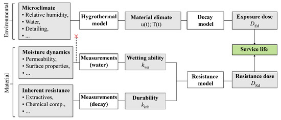
Figure 1.
An overview of how the service life of wood in above-ground applications is modelled from material and environmental influences.
Both constitutive modelling approaches and simpler empirical models have been used in the past to estimate wood moisture content in the context of performance-based design. Constitutive modelling is generally favorable, as the output includes a spatial dimension, i.e., the moisture content distribution, whereas empirical models (e.g., Ref. [22]) are limited to wood moisture content at a specific depth. While constitutive models can be used for detailed assessment, they are not easily implemented as part of any digital design guideline, as calculations are complex, time-consuming, and rely on commercial software.
The aim of this study was to evaluate a modified method for service-life prediction of wood suitable for implementation in a digital design guideline. In the present study, the proposed moisture prediction model targets two effects, namely the effect of climate and detailing, and is based on a semi-empirical model (SMM) for estimating wood moisture content in details, originally developed in [23]. The moisture content is determined as the sum of two terms, one describing the moisture content of a reference design and the other describing the effect of a specific detail. The latter has been fitted to data through regression, hence the term semi-empirical. The performance of the SMM is compared to a finite element model (FEM) developed in [24]. This is done by calculating the moisture content variation and the time until onset of decay of a specific detail exposed to various European climates. The onset of decay is estimated through two different dose-response models, namely the simplified logistic model (SLM) and the logistic model (LM). The utility of the SMM is demonstrated by calculating the time until onset of decay of four different details. Finally, it is demonstrated how factors can be derived based on the SMM combined with the SLM.
2. Materials and Methods
2.1. Detail Type
The geometry used for the comparison between the FEM and the SMM is a horizontal member (22 × 90 mm2) that is partially prevented from drying out by a vertical member (45 × 90 mm2) connected without a gap (see Figure 2). As a typical moisture trap, precipitation will cause wetting of the interface between the two members which is then unable to dry out, resulting in a small volume of damp wood surrounding the interface area. In the present paper, due to limitations with modelling end-grain absorption numerically, only the moisture content of the horizontal board is modelled for the comparison between the FE and SE model. Both end-grain faces of the horizontal board are sealed in the model, which represents a long board without drying effects from end-grain.
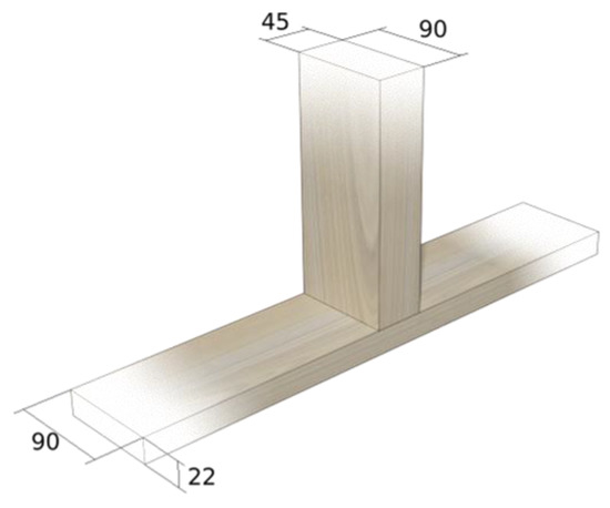
Figure 2.
The type of joint used in the present study.
2.2. Weather Data
The detail in question was modelled in about 300 different locations scattered across Europe. The locations were selected to describe a wide variety of European climates. A normal (typical) year of annual weather data was obtained for each location through the Meteonorm database [25]. The normal year is derived from a statistical model which is based on about 20 years of historical weather records. Data include hourly values of precipitation (p), temperature (T), and relative humidity (Φ).
2.3. Modelling Wood Moisture Content
Wood moisture content is calculated by the FEM and SMM. The two models are described briefly in Section 2.3.1 and Section 2.3.2, respectively, and more detailed descriptions can be found in [23,24].
2.3.1. Finite Element Model (FEM)
The numerical model is based on Fick’s second law of diffusion where the internal wood moisture transport is described by the moisture gradient and the diffusion coefficient. In two dimensions, it can be written as follows:
where u (kg/kg) is the moisture content and Du (m2/s) is a diagonal matrix with transport coefficients in the longitudinal and transverse orientations. The change in moisture content due to the exchange of moisture between the wood surface and the environment, q (kg/kg), is described as follows:
where Δpv (Pa) is the difference in vapor pressure between the wood surface and the surrounding air, (kg/m3) is the wood density, and kp (kg/m2sPa) is the mass-transfer coefficient.
Each parameter used for the numerical model is given in Table 1 and Figure 3. The diffusion coefficient is dependent both on wood moisture content and temperature. In the present study, the moisture-dependent diffusion coefficients were obtained from [26]. The diffusion coefficients were then adjusted for variations in temperature as follows:
where EA (J/mol) is the activation energy, R (J/Kmol) is the universal gas constant, and T (K) is the temperature. The activation energy was obtained from measurements based on [27]. The mass-transfer coefficient kp (kg/m2sPa) was taken from [28]. For simplicity, a constant mass-transfer coefficient was used. When the wood is exposed to liquid water, it is assumed that the outermost wood fibers instantly attain a maximum value of 120% moisture content. The relationship between relative humidity, Φ, and equilibrium moisture content, ueq, is described by the sorption isotherm, which was taken from [24]. The hygroscopic part of the sorption isotherm extended to Φ = 99% and was then interpolated to u = 120% at Φ = 100%. The temperature of the wood surface and air were assumed equal, so the difference in vapor pressure, Δpv, was calculated as the product of the saturation vapor pressure and the difference between the relative humidity of the air and the equilibrium-relative humidity of the wood surface, the latter being obtained from the sorption isotherm.

Table 1.
Parameters used in the numerical model.
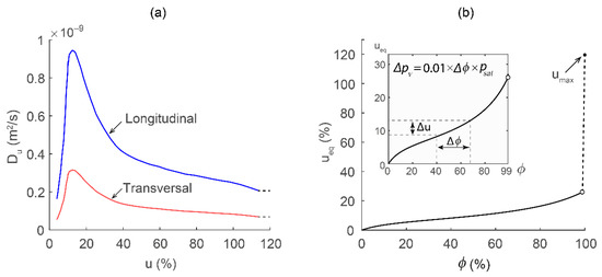
Figure 3.
Diffusion coefficients at 20 °C (a) and sorption isotherm (b). Dashed lines indicate the segments which have been subject to interpolation or extrapolation.
Due to symmetry reasons, only half the horizontal board was modelled. Boundary conditions were modelled according to Figure 4. The boundary condition between horizontal and vertical boards (moisture trap) was modelled as conditional with absorption during periods with rain and zero flux in the absence of rain, allowing for wetting due to rain but zero drying. The upper surface of the board was exposed to rain but free to exchange moisture with the ambient climate, whereas the lower surface was protected from rain. The ends of the specimen were assigned a zero-flux boundary condition to represent a long board without end-grain drying effects. Reliably modelling end-grain absorption was not possible using this type of FE model.
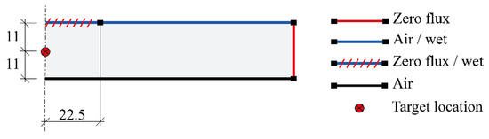
Figure 4.
Geometry and boundary conditions used by the FEM. The point used for comparison with the SMM is denoted as target location.
The input passed to the FEM consisted of weather data. The model then returned the moisture distribution in each time step. The empirical model, however, has only been calibrated for daily averages at a specific depth. As such, only the daily average moisture content near the joint in the center of the horizontal member (see marker in Figure 4, hereafter referred to as the target location) was used for the comparison.
2.3.2. Semi-Empirical Model (SMM)
The SMM considers the daily average moisture content as the sum of two independent parts:
where uref(t) is the reference moisture content variation and utrap(t) is the increase in moisture content stemming from moisture trapping. The reference moisture content variation describes the moisture content of a horizontal member without any moisture trapping effects, e.g., the horizontal member in Figure 2 without any influence of the vertical member. It can be calculated either numerically or through a separate empirical equation. Here, uref(t) was taken from the FE model. Consequently, the difference between the two models is strictly limited to how they account for the effect of moisture trapping, as described by the term utrap(t). Moisture trapping effects were here considered by superimposing utrap(t) onto the reference moisture content variation. The value of utrap was assumed to increase on days with significant precipitation, remain constant on days with only minor precipitation, and decrease on days with limited or no precipitation.
The change in utrap on days with precipitation (p > 2 mm) was set to 0.01 or 0.03 depending on if moisture absorption occurred through side-grain or end-grain. This value is hereafter referred to as Δuwet. The change of utrap on days with minor precipitation (0.5 mm ≤ p ≤ 2 mm) was set to zero. Finally, the change in utrap on days without precipitation (p < 0.5 mm) was calculated as follows:
where the parameter λ depends on daily average temperature and kdry is a detail-specific parameter which describes the conditions for drying. The value of the former was calculated as follows:
where T is the daily average temperature. For temperatures below 0 °C and above 15 °C, the value of λ was set to 1/3 and 1.0, respectively. The value of kdry for the detail in question was set to 0.07 [23]. A more detailed description of the model and how the factors were calibrated can be found in [23].
2.4. Modelling Wood Decay
Time series of wood moisture content and temperature were passed to a dose-response-function to estimate their combined effect on service life [29]. For simplicity, it was assumed that the difference between the average daily wood temperature and the average daily air temperature was negligible, and the wood temperature was thus set equal to the air temperature. The dose-response function returned daily doses, which were then summed up to an annual dose, one for each location. The annual dose was then divided by a material resistance dose, DRd, to obtain the service life in units of years, assuming that the same weather pattern is repeated.
In the present study, two different dose-response functions were used. One is the logistic model (LM) proposed by Brischke and Rapp [10], which is based on the inherent characteristics of the decay process. As fungal decay requires free water, the model has a lower threshold at 25% moisture content, below which the daily dose equals zero. The second model, hereafter referred to as the simplified logistic model (SLM), was designed without a lower threshold for moisture content [29].
The functions governing the moisture-induced dose, du, and temperature-induced dose, dT, are shown in Figure 5a,b, and the sigmoid functions describing EN 252 [30] decay rating as a function of dose are shown in Figure 5c. The daily dose, dday, is calculated by combining the moisture- and temperature-induced doses as follows:
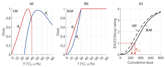
Figure 5.
Functions of moisture- and temperature-induced dose shown for the LM (a) and the SLM (b) and the sigmoid functions describing the EN 252 [30] decay rating as a function of cumulative dose (c).
As can be seen from the equations, the moisture- and temperature-induced doses vary from 0 to 1 depending on the daily average material climate conditions (u and T). The total daily dose, dday, which is a function of the temperature- and moisture-induced doses, also varies between 0 and 1, where the latter implies ideal conditions for decay. At any given point in time, the accumulated dose describes how far the decay process has progressed and is simply calculated as the cumulative sum of daily doses over the period of exposure. Since the weather input here corresponds to one year of data, the cumulative sum is referred to as the annual dose, calculated as follows:
As aforementioned, the service life, in units of years, is estimated by taking the annual dose divided by the resistance dose, dRd, which depends on wood species and treatments [20,21]. For Norway spruce (Picea abies), which is the reference species, the resistance dose, dRd, is equal to the critical dose, dcrit. In this study, the limit state is defined as the dose corresponding to the onset of decay, i.e., EN 252 [30] decay rating 1, by brown-rot fungi. The functions in Figure 5c have been fitted specifically to tests with brown-rot damage, following the methodology described in [31]. The critical dose can be determined from the sigmoid functions shown in Figure 5c to dcrit = 228 for the LM and dcrit = 284 for the SLM.
3. Results and Discussion
3.1. Comparison Between Moisture Models
Figure 6a shows the density of daily average moisture content based on the time series of all geographic locations, calculated at the target location (see Figure 4) using the FEM. Figure 6b shows the relative difference between the FEM and the SMM. As seen in Figure 6a, most locations exhibit a similar seasonal variation with higher moisture content during the winter months. At a given day, the moisture content can vary between dry (about 15%) and very moist (about 30%) depending on geographic location. At some locations, the wood remains damp over the entire year. The relative difference between the models shown in Figure 6b is also subject to a small seasonal variation. Although not shown here, this seasonal variation is related to the effect of temperature of the SMM, given by Equation (6), and disappears if this effect is neglected.
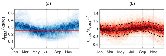
Figure 6.
Density plot of about 300 moisture-content time series calculated by the FEM with red lines marking 25% and 30% moisture content (a) and the relative difference between the two models with 80% of the data points enclosed by the dashed lines (b). Darker color indicates higher density of data.
The SLM moisture-induced dose becomes equal to one per day when the wood remains permanently above a threshold of u = 30%, implying that the moisture conditions for fungal decay remain optimal throughout the entire year. Further, it implies that a design with a higher degree of moisture trapping will not reduce the service life and that the service life is solely governed by the variations in temperature. This type of threshold is not considered in the factorized design method, as no interdependence between factors is considered. Consequently, the final product may end up being higher than the maximum limit representing optimal moisture conditions for decay.
3.1.1. Moisture Content
Figure 7 shows the results of both moisture models from four different locations together with the reference moisture variation, uref, calculated using the FEM without any moisture trap. The four locations, Verona (IT), Shkodra (AL), Haren (DE), and Aalesund, (NO) have 30, 87, 99, and 122 days with more than 2 mm precipitation, respectively, and have been selected to demonstrate the effect of precipitation on model performance. Note that the reference moisture content is a common base in both models, so the performance of the SMM is best evaluated in terms of the difference from the reference moisture variation.
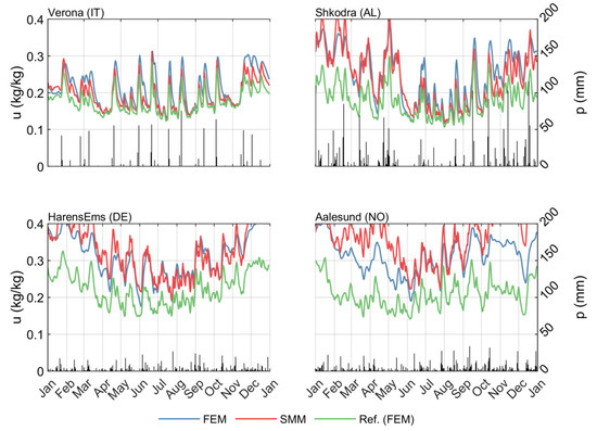
Figure 7.
Daily average moisture content in the joint calculated using the FEM (blue), the SMM (red), and the reference moisture content (green), shown together with the daily precipitation (black).
As can be seen from Figure 7, both models exhibit peaks during periods with high precipitation and converge towards the reference moisture content variation during longer periods with little or no precipitation. Qualitatively, the two models exhibit similar features with respect to both amplitude and seasonal variation. In climates with limited precipitation, the moisture variations of both models are similar to the reference moisture variation (here shown by location Verona, IT). Although not shown in Figure 7, the discrepancy between the two models tends to increase at sub-zero daily average temperature.
Figure 8 gives an indication of model consistency based on the average moisture increase due to moisture trapping, average moisture content, and days spent above 25% and 30% moisture content. In general, the SMM underestimates the average effect of moisture trapping when the effect is small and vice versa. On average, the number of days spent above 25% is higher with the FEM, but the number of days spent above 30% is higher with the SMM, indicating that the SMM is subject to higher fluctuations. These differences can be explained, to some extent, by the inherent features of the models. First, the input for the different models have different temporal resolutions, i.e., the SMM and FEM are based on daily and hourly weather data, respectively. For example, any hourly registered precipitation is included in the FEM, while daily precipitation of less than 0.5 mm is ignored by the SMM. Second, the magnitude of the peaks in the FEM are, to some extent, dampened by the inherent nature of the transport coefficient, which is decreasing at moisture contents exceeding 20%. This type of feature is not considered in the empirical model, where a fixed value is simply added to the moisture content on every day when the daily precipitation exceeds 2 mm.
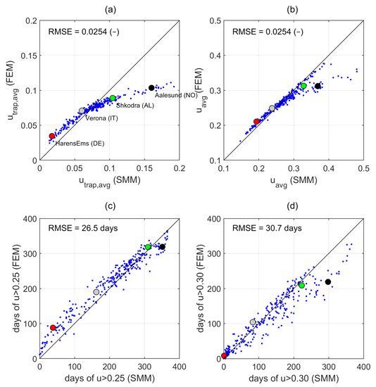
Figure 8.
Average increase in moisture content due to rain (a), average moisture content (b), days above 25% moisture content (c), and days above 30% moisture content (d), calculated with the SMM and FEM, respectively.
Finally, Figure 8 indicates that the moisture trapping effect is less dependent on cumulative annual precipitation than the number of days with precipitation when it comes to moisture trapping effect, which can be seen by comparing Shkodra (AL) and Haren (DE), where the number of days with precipitation is similar, but the annual precipitation is about 2000 mm and 800 mm, respectively. Coincidently, in previous attempts to estimate the site-specific decay potential of wood above ground, Scheffer (1971) postulated that the number of rain days plays an important role for the moisture-induced decay risk [6].
3.1.2. Annual Dose
Figure 9a,b shows a comparison between the two moisture models based on annual dose and service life (SL). To avoid having the SL tend towards infinity at near-zero dose, the reciprocal of the service life is shown here. A value of SL−1 equal to 0.1 can be interpreted as 10% of the service life being expended after one year of use.
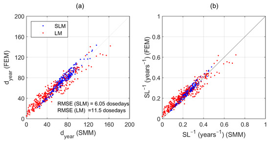
Figure 9.
Annual dose, dyear, (a) and the reciprocal of service life, SL−1, (b) in the joint calculated using the FEM and the SMM, respectively.
The two moisture models give consistent results when coupled with the SLM but differ when coupled with the LM. The inconsistency between the moisture models when coupled with the LM can be explained by the LM being more sensitive to input moisture content than the SLM. The difference is particularly pronounced in climates where the daily moisture content frequently is close to the lower limit for decay (u = 0.25), where a minor difference in moisture content can lead to significant change in daily dose. For example, at a temperature of 20 °C, a variation from 25 to 25.1% daily average moisture content will increase the LM daily dose from zero to about 0.5 and the SLM daily dose from 0.463 to 0.467.
The SLM is less sensitive to input uncertainty than the LM, as a minor difference in terms of daily average moisture content will not cause a large discrepancy in terms of the resulting daily dose. This includes uncertainty related to measurement and model errors but also uncertainty stemming from the fact that the moisture variation at the target location (see Figure 4) is not necessarily consistent with the moisture variation at the exact location where decay develops. For example, the moisture conditions in the interface between the two members in Figure 4 are likely more favorable for decay [24] than the target used in this analysis. The same issue was discussed by [32] as a problem in correlating decay progression to local moisture measurements. When making predictions based on imperfect data, there is thus a certain logic and benefit in utilizing a model which is not derived from the actual characteristics of fungal decay. The benefit of the SLM described here is, however, confined to the moisture-induced dose, as the daily average temperature is less dependent on depth from the wood surface and easier to predict.
3.2. Comparison of Decay Models
The results in the following subsections have been calculated using the SMM coupled with the LM and SLM. The performance of the horizontal board and that of the vertical board in Figure 2 have been assessed with and without sufficient air gap, see Figure 10. The values of kdry and Δuwet are based on the data from [23]. The value of kdry is higher when the joint is designed with a gap (faster drying), and the value of uwet is higher when the end-grain is exposed (increased rate of absorption and transport). The results are used as a basis for discussing the inherent differences between the LM and the SLM.
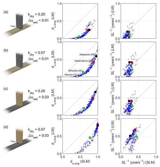
Figure 10.
Average annual moisture-induced dose (du,avg) and reciprocal of service life (SL−1) in four different types of moisture traps, calculated using the SMM coupled with the LM and SLM, respectively. From the top: exposed side-grain with gap (a) and without gap (b) and exposed end-grain with gap (c) and without gap (d). Observe that end-grain refers to the vertical member and side-grain to the horizontal member. To the left, the values for kdry and ∆uwet are shown for the investigated member.
Figure 10 shows the average annual moisture-induced dose, du,avg, and the reciprocal of service life, SL−1, in different climates for both the LM and the SLM. The value of du,avg can be interpreted as a measure of the average growth conditions for fungal decay, where 1 implies ideal conditions, without considering the effect of temperature.
Due to the inherent characteristics of the models, the SLM always indicates more favorable moisture conditions for decay than the LM. The difference is larger in climates with limited precipitation (e.g., Verona, IT) and for details with limited moisture trapping (e.g., Figure 10a). This discrepancy is related to the large discrepancy in moisture-induced dose at low moisture contents, in the region 0–25% moisture content where the LM gives a moisture-induced dose of zero.
When calculating the service life and thus taking the effect of temperature into account, the difference between the models becomes less clear. At a relatively low degree of moisture trapping (Figure 10a), the moisture content often remains below 25%, resulting in a LM dose of zero and infinite service life. For higher degree of moisture trapping (Figure 10d), the LM generally gives a shorter service life despite the moisture-induced dose being lower than for the SLM. This is due to the higher weight of temperature when combining the temperature- and moisture-induced doses (compare Equations (7) and (8)).
Factorized Design, Relative Dose
The dependency between climate and detailing has some implications for factorized design. The factors employed in previous guidelines [16,17], also referred to as relative performance, were defined as the ratio of the dose of a specific detail to the dose of the reference board, i.e., the horizontal board without moisture trap [33]. The relative performance depends on the degree of moisture trapping but also varies depending on the climate where the detail is exposed [15].
Figure 11 shows the distribution of relative performance calculated for the same four designs used previously. As can be seen from Figure 11b, the relative performance is not a useful metric when using the LM, since the moisture induced dose of the reference board is near zero at several locations, and the relative performance tends to infinity. The SLM relative performance exhibits smaller variation, with median values at approximately 1.2, 1.7, 1.7, and 2.4. These values are in good agreement with the corresponding factors given by the factorized design guideline [16], where side-grain contact with and without gap are modelled with factors of 1.2 and 1.8, respectively, and end-grain contact without gap is modelled with a factor of 2.5.
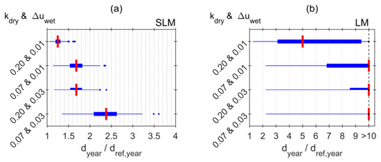
Figure 11.
Relative dose calculated using the SMM combined with the SLM (a) and LM (b) for the same four details shown in Figure 10. The red lines mark the median relative dose, the boxes extend to the 25th and 75th percentiles, the lines extend to the nonoutlier maximum and minimum, and the markers show the outliers.
Not considered by the same engineering design guideline [16] is the variability stemming from the dependency between relative performance and climate, which results in considerable uncertainty in the service-life prediction. This type of model uncertainty is avoided when multiple influencing effects (here detailing) are considered already on the basis of moisture content prior to calculating the exposure dose, as the interdependency is then considered explicitly.
3.3. Utilization and Implementation of Models
3.3.1. Estimation of Model Parameters
The parameters of the SMM can be estimated from outdoor measurements and/or through numerical simulation. Ideally, a detail is first evaluated experimentally under natural outdoor exposure over at least one year as described in [23,33]. A numerical model is then calibrated against the experimental data and used to extrapolate the results to several climates, ideally scattered across the region where the model is to be utilized. Finally, the parameter kdry of the SMM can be fitted to the larger dataset. Given sufficient confidence in the numerical model, the experimental procedure can be ignored. Alternatively, if the numerical model is not equipped to describe the detail in question, such as in the case of significant end-grain effects, then the value of kdry could be fitted directly to the experimental results, as shown in [23].
3.3.2. Implementation
The difference between previous guidelines for service-life planning of wood such as [16,17,18] and the method proposed here is twofold. Firstly, time series serve as the main input as opposed to factors. Secondly, several effects are included when calculating the moisture-content variation.
Based on the findings of the present study, the proposed model can be designed as follows. Several representative locations in the region of interest (here: Europe) are selected. For each location, the time series of daily relative humidity, temperature, and precipitation as well as pre-calculated daily values describing the reference moisture variation are obtained from a database. Alternatively, the latter time series can be replaced by an empirical model to calculate the reference moisture variation in real time from the weather data. The number of representative locations stored in the database determines the resolution of the geographic climate variations. In regions with high spatial variability in climate (such as the Alps), a higher density is desirable [34]. Based on a set of user-defined coordinates, specific time series are then interpolated, whereby the moisture content, annual dose, and service life are calculated using both the logistic and simplified logistic model. The resulting service life is presented in the form of an interval between these two values. The associated decay-model uncertainty is indicated by the size of the interval. Based on the findings of the present study, situations with few days above 25% moisture content at a depth of 10 mm from the exposed wood surface will exhibit a wider range and higher uncertainty than situations where damp conditions are dominant.
To reduce model uncertainty, future work should focus on evaluation of the current exposure model against experimental data. An ideal dataset for validation includes all the variables used in the modelling procedure, including weather data, moisture content, material temperature, and decay development. Further, the test specimens should be made of Norway spruce with controlled material properties, be mounted in non-accelerated manner with clear (or monitored) boundary conditions, and have continuous moisture data being recorded at multiple depths. Alternatively, a more practical solution is to model moisture content at a single depth and employ a numerical model to expand the spatial resolution of the results. Finally, the experiment should be performed in at least two different climates. A test setup including most of these characteristics can be found in [32].
From a practical viewpoint, it is not yet possible to include every effect on a moisture-content basis using an empirical model. This includes effects such as sheltering, local climate conditions, shading, splash water, coatings (intact versus defect), and wood species. While the ambition is to target some of these effects in future model development, any factor not included in the moisture model can still be integrated model-wise through the conventional factorized approach after calculating the annual dose. For the sake of accuracy, it is desirable to include as many effects as possible before deriving the dose, as any information regarding temporal variation is lost upon doing so.
3.3.3. In-Ground Contact
The method proposed in this study is intended for estimating the exposure dose of Norway spruce in above-ground applications subjected to intermittent wetting and drying, i.e., EN 335 [5] use-class 3, where the moisture-induced doses are largely governed by the ambient climate and the design of detailing. In the general service-life design framework, the resulting exposure dose is then combined with a material-inherent resistance dose to account for the protective properties (natural, modified, or treated) and moisture dynamics (wetting ability) of the specific material [20,21]. For terrestrial environments (use-class 4), the wood moisture content is influenced by the soil and can often be assumed to remain permanently damp [35,36].
A heuristic method to expand the existing performance-based framework to terrestrial environments may be designed on the premise that wooden members in direct contact with soil maintain moisture conditions ideal for decay. The exposure dose can then be described as a function of wood temperature, which may be determined by modelling the soil temperature. Using the same assumption, the material-inherent resistance dose is determined independent of moisture dynamics and focused on soil-contact decay tests either under laboratory or field conditions [36].
4. Conclusions
The results from the comparative assessment of different moisture and decay models clearly indicate significant differences between a factor-based approach for service-life planning with wood and the use of numerical and semi-empirical models, respectively. Within the dose-response concept we followed, it became evident that the dependency between variables is best accounted for by adjusting the wood moisture content prior to deriving the moisture-induced dose. For example, this will prevent overly conservative service-life predictions in severe environments where the moisture conditions approach optimal conditions for decay.
Considering the effect of detailing on a moisture-content basis, the two moisture models provided fairly similar results. Interpolated time series and an empirical equation for considering the effect of detailing seem to be a promising complement to the factorized approach in a digital design framework, owing largely to its low computational time.
The input moisture content should be considered when selecting the most suitable decay-prediction model. Uncertainty related to the inconsistency between the target location of moisture content (model or measured) and the optimal location for decay growth should be carefully considered. The choice of decay model becomes particularly decisive in exposure situations with low degree of moisture trapping.
To increase the accuracy of service-life prediction, future research should target verification and evaluation of existing decay-prediction models under environmental conditions with low to medium moisture-trapping effect. Until the accuracy of models has been evaluated, the uncertainty involved can be considered by calculating the service life as an interval bound between the results of several decay models.
Author Contributions
Conceptualization, J.N. and E.F.H.; methodology, All; software, J.N.; formal analysis, J.N., P.B.v.N. and C.B.; resources, J.N., C.B. and E.F.H.; data curation, J.N.; writing—original draft preparation, J.N.; writing—review and editing, J.N., C.B., P.B.v.N. and E.F.H.; visualization, J.N.; project administration, E.F.H.; funding acquisition, E.F.H. All authors have read and agreed to the published version of the manuscript.
Funding
The authors received funding in the frame of the research project CLICKdesign, which is supported under the umbrella of ERA-NET Cofund ForestValue by the Ministry of Education, Science, and Sport (MIZS)—Slovenia; The Ministry of the Environment (YM)—Finland; The Forestry Commissioners (FC)—UK; Research Council of Norway (RCN)—Norway; The French Environment and Energy Management Agency (ADEME) and The French National Research Agency (ANR)—France; The Swedish Research Council for Environment, Agricultural Sciences, and Spatial Planning (FORMAS), Swedish Energy Agency (SWEA), Swedish Governmental Agency for Innovation Systems (Vinnova)—Sweden; Federal Ministry of Food and Agriculture (BMEL) and Agency for Renewable Resources (FNR)—Germany. ForestValue has received funding from the European Union’s Horizon 2020 research and innovation programme under grant agreement N° 773324.
Data Availability Statement
Any data, raw weather data or tabulated calculated values, will be made available upon request.
Conflicts of Interest
The authors declare no conflict of interest. The funders had no role in the design of the study; in the collection, analyses, or interpretation of data; in the writing of the manuscript, or in the decision to publish the results.
References
- Brischke, C.; Bayerbach, R.; Rapp, A.O. Decay-influencing factors: A basis for service life prediction of wood and wood-based products. Wood Mater. Sci. Eng. 2006, 1, 91–107. [Google Scholar] [CrossRef]
- EN 1995-1-1. Eurocode 5: Design of Timber Structures–Part 1-1: General–Common Rules and Rules for Buildings; European Committee for Standardization: Brussels, Belgium, 2004. [Google Scholar]
- EN 460. Durability of Wood and Wood-Based Products–Natural Durability of Solid Wood–Guide to the Durability Requirements for Wood to be Used in Hazard Classes; European Committee for Standardization: Brussels, Belgium, 1994. [Google Scholar]
- EN 350. Durability of Wood and Wood-Based Products—Testing and Classification of the Durability to Biological Agents of Wood and Wood-Based Materials; European Committee for Standardization: Brussels, Belgium, 2016. [Google Scholar]
- EN 335. Durability of Wood and Wood-Based Products–Use-Classes, Definition, Application to Solid Wood and Wood-Based Products; European Committee for Standardization: Brussels, Belgium, 2013. [Google Scholar]
- Scheffer, T.C. A climate index for estimating potential for decay in wood structures above ground. For. Prod. J. 1971, 21, 25–31. [Google Scholar]
- Cornick, S.; Dalgliesh, W.A. A moisture index to characterize climates for building envelope design. J. Therm. Envel. Build. Sci. 2003, 27, 151–178. [Google Scholar] [CrossRef]
- Fernandez-Golfin, J.; Larrumbide, E.; Ruano, A.; Galvan, J.; Conde, M. Wood decay hazard in Spain using the Scheffer index: Proposal for an improvement. Eur. J. Wood Wood Prod. 2016, 74, 591–599. [Google Scholar] [CrossRef]
- Wang, C.H.; Leicester, R.; Nguyen, M. Manual 4–Decay above Ground; Tech. Rept. PN07; Forest and Wood Products Australia (FWPA): Melbourne, Australia, 2008. [Google Scholar]
- Brischke, C.; Rapp, A.O. Dose–response relationships between wood moisture content, wood temperature and fungal decay determined for 23 European field test sites. Wood Sci. Technol. 2008, 42, 507–518. [Google Scholar] [CrossRef]
- Viitanen, H.A. Modelling the Time Factor in the Development of Brown Rot Decay in Pine and Spruce Sapwood—The Effect of Critical Humidity and Temperature Conditions. Holzforschung 1997, 51, 99–106. [Google Scholar] [CrossRef]
- Nofal, M.; Kumaran, K. Biological damage function models for durability assessments of wood and wood-based products in building envelopes. Eur. J. Wood Wood Prod. 2011, 69, 619–631. [Google Scholar] [CrossRef]
- Vandemeulebroucke, I.; Caluwaerts, S.; Bossche, N.V.D. Factorial Study on the Impact of Climate Change on Freeze-Thaw Damage, Mould Growth and Wood Decay in Solid Masonry Walls in Brussels. Buildings 2021, 11, 134. [Google Scholar] [CrossRef]
- Viitanen, H.; Toratti, T.; Makkonen, L.; Peuhkuri, R.; Ojanen, T.; Ruokolainen, L.; Räisänen, J. Towards modelling of decay risk of wooden materials. Eur. J. Wood Wood Prod. 2010, 68, 303–313. [Google Scholar] [CrossRef]
- Niklewski, J.; Brischke, C.; Frühwald Hansson, E. Numerical study on the effects of macro climate and detailing on the relative decay hazard of Norway spruce. Wood Mater. Sci. Eng. 2021, 16, 12–20. [Google Scholar] [CrossRef]
- Thelandersson, S.; Isaksson, T.; Suttie, E.; Frühwald, E.; Toratti, T.; Grüll, G. Service Life of Wood in Outdoor above Ground Applications: Engineering Design Guideline–Background Document; Technical Report; TVBK-Lund University, Division of Structural Engineering: Lund, Sweden, 2011. [Google Scholar]
- Pousette, A.; Malo, K.A.; Thelandersson, S.; Fortino, S.; Salokangas, L.; Wacker, J. Durable Timber Bridges–Final Report and Guidelines; Technical Report; SP: Skellefteå, Sweden, 2017. [Google Scholar]
- Silva, A.; Prieto, A. Modelling the service life of timber claddings using the factor method. J. Build. Eng. 2021, 37, 102137. [Google Scholar] [CrossRef]
- Meyer-Veltrup, L.; Brischke, C.; Niklewski, J.; Frühwald Hansson, E.F. Design and performance prediction of timber bridges based on a factorization approach. Wood Mater. Sci. Eng. 2018, 13, 167–173. [Google Scholar] [CrossRef]
- Meyer-Veltrup, L.; Brischke, C.; Alfredsen, G.; Humar, M.; Flæte, P.-O.; Isaksson, T.; Brelid, P.L.; Westin, M.; Jermer, J. The combined effect of wetting ability and durability on outdoor performance of wood: Development and verification of a new prediction approach. Wood Sci. Technol. 2017, 51, 615–637. [Google Scholar] [CrossRef]
- Brischke, C.; Alfredsen, G.; Humar, M.; Conti, E.; Cookson, L.; Emmerich, L.; Flæte, P.; Fortino, S.; Francis, L.; Hundhausen, U.; et al. Modelling the Material Resistance of Wood—Part 2: Validation and Optimization of the Meyer-Veltrup Model. Forests 2021, 12, 576. [Google Scholar] [CrossRef]
- Frühwald, E.; Brischke, C.; Meyer, L.; Isaksson, T.; Thelandersson, S.; Kavurmaci, D. Durability of timber outdoor structures–modelling performance and climate impacts. In Proceedings of the World Conference on Timber Engineering, Auckland, New Zealand, 16–19 July 2012. [Google Scholar]
- Niklewski, J.; Isaksson, T.; Frühwald Hansson, E.; Thelandersson, S. Moisture conditions of rain-exposed glue-laminated timber members: The effect of different detailing. Wood Mater. Sci. Eng. 2017, 13, 129–140. [Google Scholar] [CrossRef]
- Niklewski, J.; Fredriksson, M. The effects of joints on the moisture behaviour of rain exposed wood: A numerical study with experimental validation. Wood Mater. Sci. Eng. 2021, 16, 1–11. [Google Scholar] [CrossRef]
- Meteonorm. Available online: www.meteonorm.com (accessed on 5 April 2016).
- Koponen, H. Dependences of moisture diffusion coefficients of wood and wooden panels on moisture content and wood properties. Paperi Ja Puu 1984, 66, 740–745. [Google Scholar]
- Koponen, H. Dependence of moisture transfer and diffusion coefficients on temperature. Paperi Ja Puu 1985, 8, 428–439. [Google Scholar]
- Wadsö, L. Surface mass transfer coefficients for wood. Dry. Technol. 1993, 11, 1227–1249. [Google Scholar] [CrossRef]
- Isaksson, T.; Brischke, C.; Thelandersson, S. Development of decay performance models for outdoor timber construction. Mater. Struct. 2013, 46, 1209–1225. [Google Scholar] [CrossRef]
- EN 252. Field Test Method for Determining the Relative Protective Effectiveness of a Wood Preservative in Ground Contact; European Committee for Standardization: Brussels, Belgium, 2014. [Google Scholar]
- Brischke, C.; Meyer-Veltrup, L. Modelling timber decay caused by brown rot fungi. Mater. Struct. 2015, 49, 3281–3291. [Google Scholar] [CrossRef]
- Meyer-Veltrup, L.; Brischke, C.; Källander, B. Testing the durability of timber above ground: Evaluation of different test meth-ods. Eur. J. Wood Wood Prod. 2017, 75, 291–304. [Google Scholar] [CrossRef]
- Isaksson, T.; Thelandersson, S. Experimental investigation on the effect of detail design on wood moisture content in outdoor above ground applications. Build. Environ. 2013, 59, 239–249. [Google Scholar] [CrossRef]
- Brischke, C.; Selter, V. Mapping the Decay Hazard of Wooden Structures in Topographically Divergent Regions. Forests 2020, 11, 510. [Google Scholar] [CrossRef]
- Marais, B.N.; Brischke, C.; Militz, H. Wood durability in terrestrial and aquatic environments—A review of biotic and abiotic influence factors. Wood Mater. Sci. Eng. 2020, 1–24. [Google Scholar] [CrossRef]
- Brischke, C.; Alfredsen, G.; Humar, M.; Conti, E.; Cookson, L.; Emmerich, L.; Flæte, P.; Fortino, S.; Francis, L.; Hundhausen, U.; et al. Modelling the Material Resistance of Wood—Part 3: Relative Resistance in above- and in-Ground Situations—Results of a Global Survey. Forests 2021, 12, 590. [Google Scholar] [CrossRef]
Publisher’s Note: MDPI stays neutral with regard to jurisdictional claims in published maps and institutional affiliations. |
© 2021 by the authors. Licensee MDPI, Basel, Switzerland. This article is an open access article distributed under the terms and conditions of the Creative Commons Attribution (CC BY) license (https://creativecommons.org/licenses/by/4.0/).