Abstract
The ecosystem services (ESs) provided by mountain regions can bring about benefits to people living in and around the mountains. Ecosystems in mountain areas are fragile and sensitive to anthropogenic disturbance. Understanding the effect of land use change on ESs and their relationships can lead to sustainable land use management in mountain regions with complex topography. Chongqing, as a typical mountain region, was selected as the site of this research. The long-term impacts of land use change on four key ESs (i.e., water yield (WY), soil conservation (SC), carbon storage (CS), and habitat quality (HQ)) and their relationships were assessed from the past to the future (at five-year intervals, 1995–2050). Three future scenarios were constructed to represent the ecological restoration policy and different socioeconomic developments. From 1995 to 2015, WY and SC experienced overall increases. CS and HQ increased slightly at first and then decreased significantly. A scenario analysis suggested that, if the urban area continues to increase at low altitudes, by 2050, CS and HQ are predicted to decrease moderately. However, great improvements in SC, HQ, and CS are expected to be achieved by the middle of the century if the government continues to make efforts towards vegetation restoration on the steep slopes.
1. Introduction
Ecosystem services (ESs) refer to the benefits gained from natural ecosystems. Due to human activities and climate change, ecosystem services undergo significant variations. Human activities, especially in terms of land use or land management change (e.g., forestry practices and agricultural practices), modify ecosystems and their spatial distribution, thereby altering the provision of ecosystem services []. Urban expansion, along with the rapid growth of the population and economy, has significantly altered regional land use patterns [], thus negatively impacting ecosystem services. Urban landscape expansion has led to losses of regional carbon storage [,], erosion prevention [], biodiversity [], and so on. Meanwhile, human activities have transformed land use to obtain desirable ecosystem services. For example, the Chinese government has launched a series of land use management practices, e.g., the Grain for Green Project (GFGP) and the Natural Forest Conservation Program (NFCP), to improve soil conservation and wildlife habitat quality []. It is necessary to have a clear understanding of how ecosystem services change over time due to human activities.
In response to human activities, the relationships between ecosystem services have also altered over time as ESs interact in a complex way []. Under the influence of urban expansion, carbon storage and habitat quality have shown simultaneous losses and caused a negative synergy between the two services []. Policies, such as GFGP, in China have led to a decrease in food production and an increase in carbon storage, thus causing a tradeoff between food production and carbon storage []. Previously, much research into the temporal and spatial pattern change of ESs and their relationships has been based on specific past years [,]. Studies at long timescales (multidecadal or multicentury) are fundamental to capturing slow social and ecological processes, which will help to manage natural resources and related ESs successfully []. Our research attempts to fully understand the past and current situation, as well as predict future scenarios for important ecosystem services in mountain regions.
Mountain regions with a large proportion of forest and grassland have significant benefits for the people living in and around the mountains. They supply resources, such as fibers, food, and fresh drinking water. Mountain forest and grass ecosystems are hotspots of carbon storage and support a large number of plant and animal species []. Therefore, they can also provide supporting services, such as soil retention and nutrient cycling, and regulating services, such as flood control, water purification, and carbon sequestration []. However, such mountain ecosystems are fragile and sensitive to anthropogenic change, so the land use changes caused by human activities modify the ESs provision []. Mountain regions are characterized by a complex topography, which leads to obvious differences in precipitation, soil, climate, and land use patterns with a change in altitude []. Therefore, the heterogeneous topography and land use landscape characteristics in mountain regions have caused the supply of ESs and their interactions to be complex []. The research on the impacts of land use change on ecosystem services and their relationships in mountain regions under complex topography should be given more attention.
A scenario analysis is a common approach used to predict the long-term effects of anthropogenic drivers on ecosystem services []. Scenarios offer a range of conditions to detect how economic development and land practices influence ecosystem services and their relationships. The CLUE-S (conversion of land use and its effects at small regional extent) model has the ability to simulate future land use change under each scenario. Water yield (WY), soil conservation (SC), carbon storage (CS), and habitat quality (HQ) are crucial for people living in this mountain region. Based on the above context, the following steps were taken in our study: (1) construct three future land use scenarios based on the existing ecological restoration policy and different socioeconomic developments; (2) quantify the impacts of land use change on WY, soil export (SE, inverse indicator of soil conservation), HQ, and CS from 1995 to 2050 (at five-year intervals); and (3) analyze the impacts of land use change on ES relationships from 1995 to 2050.
2. Materials and Methods
2.1. Study Area
Chongqing is located between 105°17′–110°11′ E and 28°10′–32°13′ N (Figure 1). It covers an area of approximately 82,400 km2. The elevation ranges from 53 to 2778 m, with high topographic relief. This region exhibits diversified geomorphic types, which include mountainous areas (75.9%), hilly areas (18.2%), and flat areas (only 5.8%). The climate is a typical subtropical monsoon climate with an annual average temperature of 17 °C. The annual average precipitation is 1200 mm, with the rainy season lasting from April to September. Chongqing is the newest of the four municipalities under the direct leadership of the central government and the largest economic center in the upper reaches of the Yangtze River. The Yangtze River runs southwest to northwest through Chongqing. As a tributary, the Jialing River joins it at the center.
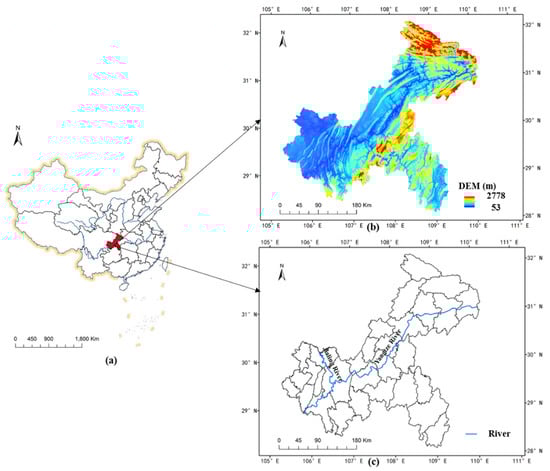
Figure 1.
Location (a), digital elevation model (DEM) (b), and rivers (c) of the study area.
Soil erosion in Chongqing has been serious as approximately 15% of its cropland has a slope of >25°. To effectively control soil loss, the Chinese government initiated the GFGP (Grain for Green program), converting cropland on steep slopes to forest and grassland, in 2000. Therefore, it is one of the key areas of the Grain for Green Program. This mountain region has experienced remarkable urban expansion since 1997, with the urbanization rate increasing from 31% to 62%. Chongqing has experienced major changes in its environment and landscape due to the implementation of ecological projects, socioeconomic development, and climate change. The regional ESs have been altered remarkably.
2.2. Data Sources
The Integrated Valuation of Ecosystem Services and Tradeoffs (InVEST) and Universal Soil Loss Equation (USLE) models were employed to assess the four ESs. Spatial map datasets and specific biophysical tables were required as inputs. Four types of data were used in our study: (1) land use map, (2) climate data, (3) soil data, and (4) digital elevation model data. A detailed description of these data is given in Table 1.

Table 1.
Description of the datasets adopted in this study.
2.2.1. Ecosystem Services Selection
Regulating and supporting ES indicators, such as soil conservation, carbon storage, and habitat quality, are of particular relevance in mountainous regions due to their unique topography and high vegetation coverage. Soil erosion control is of particular concern to local stakeholders as Chongqing suffers from severe soil erosion. The carbon storage is huge in this region and plays an important role in the global carbon balance as a carbon sink. The quantity of water discharge is particularly relevant in terms of the local and downstream flood and drought risk, as Chongqing is in the upper reaches of the Yangtze River. Based on the above reasons, four key ecosystem services (i.e., WY, SC, CS, and HQ) were selected for this research.
2.2.2. Ecosystem Services Assessment
Four types of ecosystem services were assessed, and each ecosystem service was calculated using different methods (Table 2).
Table 2.
Methods for ecosystem services assessment.
2.2.3. Simulating Land Use Change from 2020 to 2050
The CLUE-S (conversion of land use and its effects at small regional extent) model, proposed based on the CLUE model, was used to simulate the future land use change under each scenario []. The CLUE-S model includes two core modules, a non-spatial demand module and a spatial allocation procedure. The changes for all land use types were first calculated in the demand module. Parameters, including land use conversion elasticity, transfer matrices, and restrictive areas, need to be set in the spatial module. According to the total probability using the binary logistic regression method, the demands are translated into land use changes at different locations within the study region using a raster-based system:
where Pn represents the probability that a certain land use type n will appear in each grid unit (values ranging between 0 and 1), X is the driving factor, and α is the regression coefficient of the driving factors. In this study, we used nine factors of land use change, including population, gross domestic product, elevation, slope, annual average precipitation, annual average temperature, distance from the river, administration center, and main road.
Land use data from 2005 were used as the input data to simulate the land use pattern of 2015, and the simulation results were compared with the actual land use map in 2015 for validation. We adopted accuracy coefficients (overall accuracy, Kappa index, producer accuracy, and user accuracy) to reflect the simulated performance. The overall accuracy (83.9%) and Kappa index (0.848) were high. User accuracy (UA) ranged from 62.3% to 93.6%, and producer accuracy (PA) ranged from 71.6% to 93.4%. The results revealed a good consistency between the simulated and actual land use maps. Appendix A shows the simulated and actual land use maps for 2015.
To explore the long-term impacts of land use change on ecosystem services, CLUE-S was used to construct land use scenarios. Two dominant drivers, including urbanization and afforestation policies, were considered in our scenario analysis. Therefore, we constructed three scenarios: (1) business as usual (BAU), (2) rapid urbanization (RU), and (3) ecological conservation (EC). Land use simulations from 2020 to 2050 were performed at five-year intervals (i.e., 2020, 2025, 2030…2050). We projected land use maps up to 2050 based on the reference year 2015.
- (1)
- Business as usual scenario. Land use change under this scenario reflects decade-long trends of land use change. The land use change patterns are similar to those from 2005 to 2015. Land use demands for 2020 to 2050 were estimated based on historical statistics of land use change from 2005 and 2015. The rate of land use change is considered to agree with the annual change from 2005 to 2015. The area of built-up land in 2050 was twice that in 2015, at the expense of cropland, woodland, and grassland. The area of cropland, woodland, and grassland decreased slowly at annual average rates of 0.07%, 0.01%, and 0.25%, respectively.
- (2)
- Rapid urbanization scenario. This scenario forecasts land use under rapid economic development and urban expansion. The area of built-up land, including rural and urban residential land and industrial land, increases rapidly. The built-up area in 2050 was set to be three times that in 2015. The increased area will come from cropland (70%), woodland (20%), and grassland (10%).
- (3)
- Ecological conservation scenario. A karst mountain region is highly desirable for preserving the natural ecosystems and increasing forest and grass coverage. Cropland is set to decrease by 20% in 2050. The cropland will be converted to woodland (70%) and grassland (30%).
3. Results
3.1. Land Use Changes from 1995 to 2050
3.1.1. Land Use Change from 1995 to 2015
Cropland and woodland were the two largest land use types in the mountain region, whereas built-up land and water bodies accounted for the smallest proportions (Figure 2). The cropland was concentrated in low altitudes (Figure 2a). It decreased slightly from 1995 to 2015, and the decrease rate was larger in high altitudes. Woodland was mainly distributed in southeast and northeast Chongqing, areas with higher altitude, and increased from 36.9% to 37.2% (Figure 2b). The grassland decreased at low altitudes, while it increased at high altitudes. Built-up land was primarily located in central Chongqing, with low altitudes, while little is seen at altitudes of >1500 m. Built-up land showed the greatest increase of 233%. Water bodies experienced an overall increase trend from 1995 to 2015.
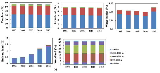
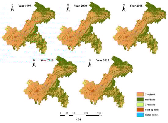
Figure 2.
Proportions of land use types at different altitude gradients from 1995 to 2015 (a). Spatial distributions of land use in Chongqing from 1995 to 2015 (b).
3.1.2. Land Use Change from 2020 to 2050 under Different Scenarios
Table 3 shows the percentage of land use types under different scenarios. In all scenarios, cropland is the dominant land use type in Chongqing in 2050. Under the BAU scenario, built-up area will increase by 110.03%, from 1.18 × 10⁵ ha in 2015 to 2.49 × 10⁵ ha in 2050. The increased built-up area will be mainly located at low altitudes. The areas of decreases in cropland and grassland are expected to concentrate at altitudes between 0 and 2000 m, while woodland will experience a decrease at altitudes between 0 and 500 m. Furthermore, woodland is expected to show an increase in northeast Chongqing at altitudes between 500 and 1000 m (Figure 3a).
Table 3.
Percentage of land use types under three scenarios.
Figure 3.
Land use maps in 2015 (baseline) and 2050 under different scenarios. Notes: EC represents ecological conser-vation (a). RU represents rapid urbanization (b). BAU represents business as usual (c). The three highlighted boxes under each scenario represent the most obvious locations of landscape conversion. The right-most column shows comparisons in the percentage of different land use types between baseline and 2050 under the three scenarios.
Rapid urban expansion is set to continue in Chongqing during 2015–2050. Built-up area will increase by 202.0%, from 1.18 × 10⁵ ha in 2015 to 3.57 × 10⁵ ha in 2050 (Figure 3b). The area of built-up land will increase, while cropland, woodland, and grassland will decline in the RU scenario. The largest growth in built-up land is expected to be mainly distributed in the central and western parts of Chongqing at low altitudes.
Under the ecological conservation scenario, GFGP policies up to the year 2050 were considered. Our simulated results indicate that woodland will increase by 18.9%, from 2.97 × 10⁶ ha to 3.53 × 10⁶ ha. Grassland will increase by 55.8%, from 3.85 × 10⁵ ha to 6.01 × 10⁵ ha. The areas of woodland and grassland increased, while cropland decreased in the EC scenario. The growth of woodland and grassland will mainly be in the central and eastern parts of Chongqing, at altitudes between 500 and 1500 m (Figure 3c). The largest declines in cropland will occur at altitudes between 500 and 1000 m.
3.2. The Impact of Land Use Change on Ecosystem Services
3.2.1. The Impact of Land Use Change on Ecosystem Services from 1995 to 2015
Ecosystem services experience temporal and spatial variations due to past land use change. Water yield was 59.06 × 10⁹ m3 in 2015, an increase of 0.13% from 1995 (Figure 4a). WY in northeast Chongqing showed the lowest value due to the relatively high vegetation cover and low precipitation. The changes in spatial distribution for WY from 1995 to 2015 are shown in Figure 5. WY showed a great increase in the central area but a significant decrease in the northeast. WY increased at low and high altitudes and decreased at moderate altitudes of 500–1500 m (Figure 4b). Soil conservation improved because soil export (SE) decreased by 1.68% over the past two decades, with 0.76 × 10⁸ Mg in 2015. SC showed improvements in changing areas. SE exhibited a decreasing trend at altitudes of 0–1500 m and an increasing trend at altitudes of >1500 m. Carbon storage and habitat quality increased slightly at first and then decreased significantly from 1995 to 2015. Improvements in CS and HQ were seen in northeast Chongqing at altitudes between 500 and 1500 m (Figure 5), while declines were seen in the western part at altitudes of 0–500 m and >2000 m. These two services showed similar spatial distribution patterns, with the highest values in the southeast and northeast Chongqing and the lowest values in the central part.
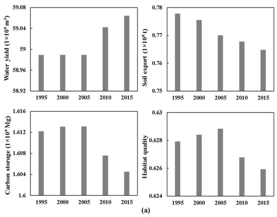
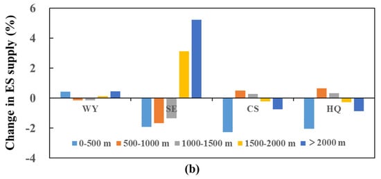
Figure 4.
Variations in ecosystem services provision from 1995 to 2015 (a). Changes in ESs of past land use distribution (1995) in relation to current ESs (2015) at different altitudes (b). Negative change indicates a decline in specific ES, while positive change presents an increase in specific ES in (b).
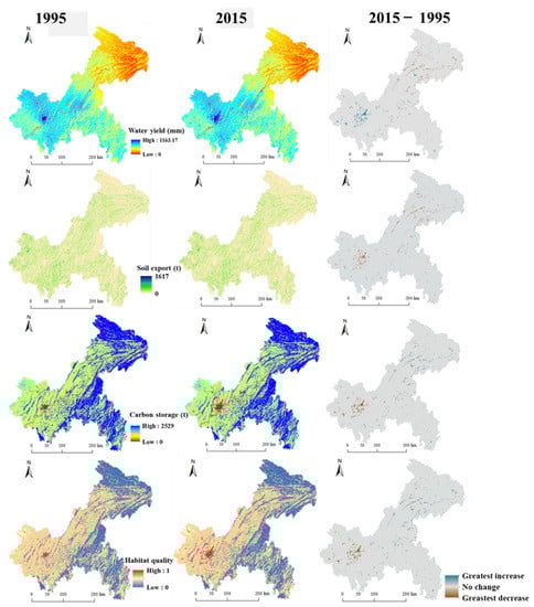
Figure 5.
Spatial distributions of WY, SE, CS, and HQ in 1995 and 2015. The right-most column represents the changing areas of the four ESs.
3.2.2. Ecosystem Services Changes Based on Future Land Use Scenarios
Land use in 2015 was chosen as the baseline for comparison, and 2020–2050 was simulated under the three scenarios. The change in the provision of ecosystem services is shown in Figure 6. The ecosystem services showed great differences under the three scenarios. The ecosystem services under the RU scenario are comparable to those under the BAU scenario. The ecosystem services under the EC scenario, however, showed great differences from those under the RU and BAU scenarios. The ecological conservation scenario led to declines in water yield (−1.5%) and soil export (−17.7%) due to forest expansion and a great improvement in habitat quality (+7.0%) and carbon storage (+5.9%). In contrast, habitat quality and carbon storage under the RU scenario decreased by 2.5% and 2.6%. Water yield increased as a result of the expansion of built-up area. Carbon storage and habitat quality under BAU decreased by 0.8% and 1.1% compared to the baseline.
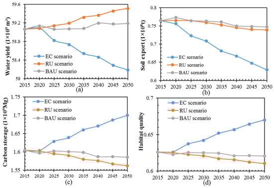
Figure 6.
Trends of ecosystem services from 2020 to 2050 (at five-year intervals) under the three scenarios. EC represents ecological conservation. RU represents rapid urbanization. BAU represents business as usual. The changes in the provision of water yield (a), soil export (b), carbon storage (c), and habitat quality (d) under the three scenarios from 2020 to 2050.
The changes in the supply of ecosystem services showed great differences at different altitudes (Figure 7). Compared to 2015, WY in 2050 showed a decreasing trend at all altitudes under the EC scenario, while it exhibited increases at low altitudes and declines at high altitudes under the BAU and RU scenarios. SE in 2050 showed a great decrease at all altitudes and in all scenarios compared to the baseline. The decrease in SE under the EC scenario was enhanced with the increase in altitude, ranging from 5% to 72%. In the BAU and RU scenarios, the declines in SE were greater at high altitudes and smaller at low altitudes. CS under the EC scenario showed large increases at all altitudes, and larger increases were found at altitudes between 500 and 1000 m and >2000 m. CS under the BAU and RU scenario decreased at low altitudes and increased at high altitudes, while the decrease at low altitudes was greater under RU than under BAU. HQ showed similar change trends to CS at different altitudes under the EC scenario. Furthermore, great declines in HQ were found at low altitudes under both the BAU and RU scenarios.
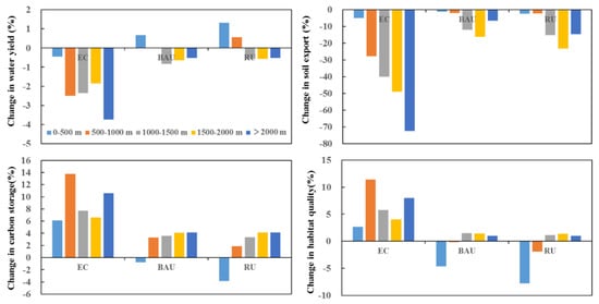
Figure 7.
The changes in ecosystem services under the three scenarios at different altitudes. Negative changes indicate a decline in specific ES in a specific scenario, while positive changes present an increase in specific ES in a specific scenario.
3.3. The Impact of Land Use Change on Relationships between Ecosystem Services
3.3.1. The Impact of Land Use Change on Relationships between Ecosystem Services from 1995 to 2015
Relationships between ecosystem services were first assessed for the whole region (denoted by black triangles in Figure 8) and then at different altitudes (denoted by colored dots) by conducting a Pearson’s correlation analysis grid by grid. All pairs of ESs were significantly correlated from 1995 to 2015 (P < 0.01). WY showed persistent tradeoffs with soil conservation (SC), indicated by positive correlations between WY and SE (an inverse indicator of SC). WY and SC were weakly correlated (0 ≤ |r| < 0.3), and this weak relationship intensified as the altitude increased. The tradeoff between WY and SC was strongest at altitudes >2000 m (represented by dark blue dots). As to the relationships between WY and CS, HQ remained consistently negative. WY and CS showed weak tradeoffs at altitudes of 0–500 m (0 ≤ |r| < 0.3), moderate tradeoffs at altitudes of 1000–2000 m (0.3 ≤ |r| < 0.5), and strong tradeoffs at altitudes of 500–1000 m and >2000 m (|r| ≥ 0.5). WY and HQ showed moderate tradeoffs at altitudes of 1000–2000 m and strong tradeoffs at other altitudes. SC showed synergies with CS and HQ, indicated by negative correlations between SE and CS or HQ. The synergy between SC and CS intensified at high altitudes. The synergies between SC and HQ were weak at low altitudes and moderate at altitudes >500 m. CS and HQ showed a consistently strong positive relationship at all altitudes, while this relationship was relatively weak at low altitudes.
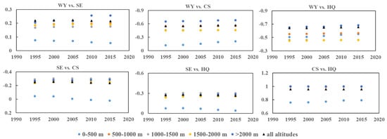
Figure 8.
The relationships between ecosystem services from 1995 to 2015. Notes: XX vs. XX represents the relationship of XX and XX (i.e., WY vs. CS indicated the relationship between WY and CS, the same as below). The different colored dots represent the relationships between ecosystem services at different altitudes. The black triangles indicate the relationships between ecosystem services for the whole region. The numbers on the Y-axis are the Pearson’s correlation coefficients between pairs of ESs.
3.3.2. The Relationships between Ecosystem Services Based on Future Land Use Scenarios
The variations in relationships between ecosystem services from 2020 to 2050 in different scenarios are shown in Figure 9. The changes in the relationship between ecosystem services under the RU scenario are similar to those under the BAU scenario. Tradeoffs between WY and SC varied slightly in different scenarios. This tradeoff was weakest at altitudes of <500 m (represented by light blue dots in Figure 9), decreased with the increase of altitude between 500 and 2000 m, and was strongest at altitudes of >2000 m in the BAU and RU scenarios. Furthermore, such a tradeoff was intensified at altitudes of <500 m and diminished at other altitudes in the EC scenario. WY showed a moderate tradeoff with CS; this tradeoff was intensified slightly in the BAU and RU scenarios and diminished in the EC scenario. The relationship between WY and CS showed a large variation in different altitudes. Such a relationship was weak at altitudes of <500 m, diminished with the increase in altitude between 500 and 2000 m, and was strong at altitudes of >2000 m in the BAU and RU scenarios. The strength of the tradeoff between WY and CS was diminished at all altitudes except for <500 m in the EC scenario. The tradeoff between WY and HQ was strengthened in the RU scenario and weakened slightly in the EC scenario. WY and HQ were correlated at altitudes of 0–1000 m and >2000 m, and moderately at altitudes of 1000–2000 m in the BAU and RU scenarios. The strength of the negative relationship between WY and HQ diminished at different altitudes in the EC scenario.
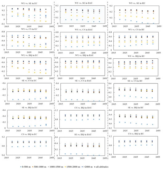
Figure 9.
Variation of the relationship between ecosystem services from 2020 to 2050. Notes: EC represents ecological conservation (right-most column). RU represents rapid urbanization. BAU represents business as usual. WY refers to water yield, SE to soil export, CS to carbon storage, and HQ to habitat quality. WY vs. CS in EC represents the relationship between water yield and carbon storage in the ecological conservation scenario. The different colored dots represent the relationships between ecosystem services at different altitudes. The black triangles indicate the relationships between ecosystem services for the whole region. The numbers on the Y-axis of each figure are the Pearson’s correlation coefficients between pairs of ESs.
4. Discussion
4.1. Effect of Land Use Change on Ecosystem Services
In recent decades, the land use pattern in our research area has experienced great variation due to rapid urbanization and the implementation of large-scale ecological restoration. In line with previous studies, we found that the changes in land use pattern have great impacts on the supply of ESs [,]. In mountain regions, the impact of land use change on ESs is closely related to topography []. The increased WY mainly occurred at low altitudes. In these areas, the conversion of cropland to built-up land due to urban expansion increased the impervious area, thereby increasing WY. During the past few decades, rapid urban expansion has also led to simultaneous losses of CS and HQ at low altitudes (similar to []). The implementation of large-scale ecological restoration, such as GFGP in the Yangtze and Yellow River basins, has fundamentally improved regulating and supporting services (e.g., SC, water purification, and flood control) []. In areas at altitudes of 1000–1500 m, a large amount of cropland was converted to woodland due to the implementation of GFGP, which enhanced SC, CS, and HQ.
Scenario analyses can clearly predict the long-term impact of future specific land use changes on ecosystem services. Urban expansion has been a common phenomenon from the regional to global scales in recent decades and will likely continue in the future. Due to persistent urbanization, urban area will take up more former cropland, which will have negative impacts on ecosystem services [,]. In the RU scenario, we predicted that, by 2050, the urban area will increase at low altitudes due to the constraints of terrain conditions, which will lead to the degradation of CS and HQ. In this process, the flood risk caused by extreme precipitation will increase as it belongs to the monsoon climate zone. However, if the government continues to implement ecological restoration, great improvements in ESs will be achieved by the middle of the century. Converting cropland on steep slopes to forest and grassland will be an important way to control soil erosion in mountain regions []. In the BAU scenario, the land use change patterns are similar to those from 2005 to 2015. Chongqing is the core area of the Three Gorges Reservoir (TGR) Area. The Three Gorges Dam (TGD), located in the upper valley of the Yangtze River, is the world’s largest hydroelectricity project. It was completed in 2009 and put into use after the trial operation from 2003 to 2010. The backwater area of the TGR extends to the city of Chongqing. Therefore, the water body in BAU is expected to change slightly by 2050 as its increase was caused by the impoundment of the TGR from 2005 to 2015. In the BAU scenario, if current trends continue, over the period 2015–2050, the urban area and water bodies will continue to increase at low altitudes, and GFGP will continue to be implemented. As a result, CS and HQ in CQ will gradually decrease.
4.2. Effect of Land Use Change on Relationships between Ecosystem Services
Land use change can affect the supply of ESs, thus leading to changes in their relationships. In line with previous studies [,], provision services showed tradeoffs with supporting and regulating services (i.e., the negative relationships between WY and SC, HQ, and CS), while supporting services showed synergies with regulating services (i.e., the positive relationships between SC and HQ, CS). Six pairs of ecosystem services experienced slight variations in our study during 1995–2015. This is because urban expansion and ecological restoration are the two main drivers of land use change. Although rapid urbanization has resulted in losses of ESs, ecological restoration is also being implemented in our study area, and the ES provided by the implementation of ecological restoration can offset the loss of ESs []. Our scenario analysis results suggest that rapid urbanization will gradually intensify the tradeoffs of WY vs. HQ and WY vs. CS, while decreasing the synergies of SC vs. CS and SC vs. HQ. The GFGP can enhance the synergies between SC and CS and HQ, which indicates simultaneous increases in these ESs with the implementation of GFGP. This is because vegetation restoration on steep slopes can control soil loss effectively [], improve carbon storage, and maintain biodiversity [].
The changes in relationships between ESs showed large variations with altitude. Altitude plays a key role in mountain regions. Tradeoffs related to WY were intensified with an increase in altitude. A large proportion of forest at higher altitudes can provide more supporting and regulating services. However, the evapotranspiration and interception of forests consume a large proportion of precipitation, thus decreasing water yield at high altitudes []. Therefore, WY was the lowest at high altitudes with high forest cover, and other services (i.e., SC, HQ, and CS) were the greatest. The relationships of SC vs. CS and SC vs. HQ showed the highest synergy at altitudes of 1000–1500 m. Previous research in the Yangtze River basin showed that the most important contributor to soil erosion is farming on steep slopes at relatively high altitudes []. Large proportions of cropland and forest were distributed at altitudes of 1000–1500 m, and these areas are hotspots of food supply, soil control, carbon storage, and biodiversity.
4.3. Management Implications
The results of the scenario analysis offer guidance for long-term policy development. Firstly, the mountains are mostly distributed in the northeast and southeast of Chongqing, where more severe soil erosion occurs due to the steep slopes and heavy rainfall. This study has proven that the EC scenario can significantly reduce soil loss. Thus, GFGP should be continued in Chongqing, especially in its southeast and northeast regions. Secondly, if changes in land use follow the transition patterns of the past decade, ESs are predicted to decrease slightly in the BAU scenario. Optimizing land use allocation is of great importance for improving ecosystem services in mountain regions. Vegetative buffer strips in riparian areas have been proven to be efficient for reducing runoff and soil export, increasing landscape connectivity, and protecting biodiversity, even if small in extent []. As for the upper reaches of the Yangtze River, setting buffer strips along the main stream and tributaries can be considered a relatively optimal land allocation. Finally, the RU scenario shows some degradation in the provision of ESs. The expansion of urban areas is predicted to occur in central and west Chongqing. Thus, local governments in the western and central regions need to balance economic development and ecological conservation. We suggest that the spread of urban areas needs to be well planned. For example, new urban areas should maintain a certain proportion of woodland and grassland.
4.4. Limitations and Future Studies
Our research still has some limitations. First, only four ESs were investigated, which cannot reflect the overall impacts caused by land use change. Especially in terms of food supply, previous research has indicated that a decrease of farmland due to the implementation of GFGP threatens food security and puts economic pressure on local people []. Mountain regions also have aesthetic significance for local residents and tourists []. Therefore, cultural services are also important and should be assessed in a future study. Secondly, the projection of future land use by the CLUE-S model is based on historical land use change patterns. Land use change could be affected by natural, economic, social, and policy factors, so it remains uncertain []. Extreme natural or economic events and sudden policy shifts may alter the magnitude of land use conversions in the future []. For instance, the TGR was impounded to a maximum elevation of 175 m, leading to an overall increase in the area of the water body. A special zone, the hydro-fluctuation belt (HFB), has been created by the seasonal impoundment of the TGR area. This belt has a total area of 349 km2, with a vertical height of 30 m along the Yangtze River backwater area. The HFB is covered by water body in the impounding period and bare land or cropland in the discharging period. This conversion in land use cannot be simulated by the CLUE-S model. To reflect more realistic land use change, we should explore how to take extreme condition and policy factors into account in the simulation process. In addition, the accuracy of built-up land had the lowest value among different land use types, which may be due to the small proportion and scattered nature of built-up land. Thus, we should pay more attention to built-up land simulations. During the simulation process in the EC and RU scenarios, rivers in Chongqing were considered restricted areas that remain unchanged. Furthermore, several policies on ecological protection have been implemented by central and local governments, such as “Ecological Function Zoning”, “the Nature Reserves”, and “Ecological Red Lines”. The existing policies were employed to delimit the protected areas. However, these protected areas were not considered restricted areas in our study due to a lack of data. In a future study, all the protected areas (i.e., woodland, grassland) should be fully delimited and considered as restricted areas when running the CLUE-S model. Finally, the uncertainty of the input parameters contained in the land use simulation process should be quantified in a future study. Sensitivity analysis has been proven to be useful for identifying the main sources of uncertainty and improving the accuracy of land use simulation models [].
5. Conclusions
The impact of past and future land use changes on ecosystem services and their relationships in a mountain region were investigated in our study. From 1995 to 2015, the land use in Chongqing experienced major changes due to ecological projects and rapid urbanization. Accordingly, ESs experienced temporal, spatial, and altitude variations. WY experienced an overall increase, with a great increase in the central area and a significant decrease in the northeast. SC improved as soil export led to a decrease in changing areas. CS and HQ increased slightly at first and then decreased significantly. Based on existing policies and socioeconomic development, the long-term effects of land use change on ESs by 2050 were explored by setting up several land use scenarios. Rapid urbanization will lead to decreases in HQ and CS, intensify the tradeoffs of WY vs. CS and HQ, and decrease the synergies of supporting and regulating services. However, great improvements in SC, HQ, and CS in the EC scenario are expected to be achieved by the middle of the century if the government continues to implement vegetation restoration on steep slopes. Furthermore, CS and HQ in the BAU scenario will gradually decrease if the current trends continue until 2050. The results offer guidance for long-term policy development in mountain regions.
Author Contributions
Conceptualization, J.G. and X.T.; methodology, H.B. and S.L.; software, S.L.; formal analysis, H.B.; writing—original draft preparation, J.G. All authors have read and agreed to the published version of the manuscript.
Funding
This research is funded by the National Natural Science Foundation of China (No. 41701611, 41830648), the Fundamental Research Funds for the Central Universities (No. XDJK2019C090), and the General program of social science and planning of Chongqing (No. 2020YBZX15).
Conflicts of Interest
The authors declare no conflict of interest.
Appendix A
The accuracy for land use simulation.
The overall accuracy and kappa index between simulated and actual land use maps for 2015 are 83.9% and 0.848, which reveals a good consistency between the simulated and actual land use maps. User accuracy (UA) ranged from 71.6% to 93.4%, and producer accuracy (PA) ranged from 62.3% to 93.6% (Table A1).
Table A1.
Confusion matrix between simulated and actual land use map in 2015.
Table A1.
Confusion matrix between simulated and actual land use map in 2015.
| Simulated Land Use Map (Unit: Pixel) | Producer Accuracy (%) | Kappa Index | ||||||
|---|---|---|---|---|---|---|---|---|
| Actual Land Use Map | Cropland | Woodland | Grassland | Built-Up Land | Water Body | Total | ||
| Cropland | 465220 | 23169 | 6326 | 2725 | 485 | 497925 | 93.4 | |
| Woodland | 22139 | 302925 | 2023 | 2189 | 382 | 329658 | 91.9 | |
| Grassland | 6658 | 2919 | 32646 | 471 | 128 | 42822 | 76.2 | |
| Built-up land | 2136 | 986 | 546 | 9421 | 66 | 13155 | 71.6 | |
| Water body | 756 | 104 | 185 | 304 | 8460 | 9809 | 86.2 | |
| Total | 496909 | 330103 | 41726 | 15110 | 9521 | 893369 | Overall Accuracy | |
| User Accuracy (%) | 93.6 | 91.8 | 78.2 | 62.3 | 88.9 | 83.0 | 83.9 | 0.848 |
Notes: Produce accuracy is the probability of a pixel S(x,y) in a simulated land use map consistent with its corresponding pixel T(x,y) in an actual land use map. User accuracy is the probability of a pixel S(x,y) in an actual land use map consistent with its corresponding pixel T(x,y) in a simulated land use map.

Figure A1.
Comparison between the simulated (a) and actual land use map (b) in 2015.
References
- Polasky, S.; Nelson, E.; Pennington, D.; Johnson, K.A. The Impact of Land-Use Change on Ecosystem Services, Biodiversity and Returns to Landowners: A Case Study in the State of Minnesota. Environ. Resour. Econ. 2010, 48, 219–242. [Google Scholar] [CrossRef]
- Seto, K.C.; Güneralp, B.; Hutyra, L.R. Global forecasts of urban expansion to 2030 and direct impacts on biodiversity and carbon pools. Proc. Natl. Acad. Sci. USA 2012, 109, 16083–16088. [Google Scholar] [CrossRef]
- Delphin, S.; Escobedo, F.; Abd-Elrahman, A.; Cropper, W. Urbanization as a land use change driver of forest ecosystem services. Land Use Policy 2016, 54, 188–199. [Google Scholar] [CrossRef]
- He, C.; Zhang, D.; Huang, Q.; Zhao, Y. Assessing the potential impacts of urban expansion on regional carbon storage by linking the LUSD-urban and InVEST models. Environ. Model. Softw. 2016, 75, 44–58. [Google Scholar] [CrossRef]
- Zhang, Y.; Liu, Y.; Zhang, Y.; Liu, Y.; Zhang, G.; Chen, Y. On the spatial relationship between ecosystem services and urbanization: A case study in Wuhan, China. Sci. Total Environ. 2018, 637–638, 780–790. [Google Scholar] [CrossRef] [PubMed]
- Xie, W.; Huang, Q.; He, C.; Zhao, X. Projecting the impacts of urban expansion on simultaneous losses of ecosystem services: A case study in Beijing, China. Ecol. Indic. 2018, 84, 183–193. [Google Scholar] [CrossRef]
- Liu, J.; Li, S.; Ouyang, Z.; Tam, C.; Chen, X. Ecological and socioeconomic effects of China’s policies for ecosystem services. Proc. Natl. Acad. Sci. USA 2008, 105, 9477–9482. [Google Scholar] [CrossRef]
- Bennett, E.M.; Peterson, G.D.; Gordon, L.J. Understanding relationships among multiple ecosystem services. Ecol. Lett. 2009, 12, 1394–1404. [Google Scholar] [CrossRef] [PubMed]
- Lang, Y.; Song, W. Quantifying and mapping the responses of selected ecosystem services to projected land use changes. Ecol. Indic. 2019, 102, 186–198. [Google Scholar] [CrossRef]
- Sun, X.; Lu, Z.; Li, F.; Crittenden, J.C. Analyzing spatio-temporal changes and trade-offs to support the supply of multiple ecosystem ser-vices in Beijing, China. Ecol. Indic. 2018, 94, 117–129. [Google Scholar] [CrossRef]
- Schirpke, U.; Tscholl, S.; Tasser, E. Spatio-temporal changes in ecosystem service values: Effects of land-use changes from past to future (1860–2100). J. Environ. Manag. 2020, 272, 111068. [Google Scholar] [CrossRef]
- Gratzer, G.; Keeton, W.S. Mountain Forests and Sustainable Development: The Potential for Achieving the United Na-tions’ 2030 Agenda. Mt. Res. Dev. 2017, 37, 246–253. [Google Scholar] [CrossRef]
- Payne, D.; Spehn, E.M.; Snethlage, M.; Fischer, M. Opportunities for research on mountain biodiversity under global change. Curr. Opin. Environ. Sustain. 2017, 29, 40–47. [Google Scholar] [CrossRef]
- Chaudhary, S.; Tshering, D.; Phuntsho, T.; Uddin, K.; Shakya, B.; Chettri, N. Impact of land cover change on a mountain ecosystem and its services: Case study from the Phobjikha valley, Bhutan. Ecosyst. Heal. Sustain. 2017, 3, 1393314. [Google Scholar] [CrossRef]
- Deng, C.; Liu, J.; Nie, X.; Li, Z.; Liu, Y.; Xiao, H.; Hu, X.; Wang, L.; Zhang, Y.; Zhang, G.; et al. How trade-offs between ecological construction and urbanization expansion affect ecosystem services. Ecol. Indic. 2021, 122, 107253. [Google Scholar] [CrossRef]
- Mengist, W.; Soromessa, T.; Legese, G. Ecosystem services research in mountainous regions: A systematic literature review on current knowledge and research gaps. Sci. Total Environ. 2020, 702, 134581. [Google Scholar] [CrossRef] [PubMed]
- Tallis, H.; Kareiva, P.; Marvier, M.; Chang, A. An ecosystem services framework to support both practical conservation and economic development. Proc. Natl. Acad. Sci. USA 2008, 105, 9457–9464. [Google Scholar] [CrossRef]
- Budyko, M.I.; Miller, D.H.; Miller, D.H. Climate and Life; Academic Press: New York, NY, USA, 1974. [Google Scholar]
- Sharp, R.; Tallis, H.T.; Ricketts, T. VEST 3.3.3 User’s Guide; The Natural Capital Project: Stanford, CA, USA, 2014. [Google Scholar]
- Wischmeier, W.H.; Smith, D.D. Predicting Rainfall Erosion Losses: A Guide to Conservation Planning. In USDA Agricultural Handbook; USDA: Washington, DC, USA, 1978. [Google Scholar]
- Tappeiner, U.; Tasser, E.; Leitinger, G.; Cernusca, A.; Tappeiner, G. Effects of historical and likely future scenarios of land use on above- and belowground vegetation carbon stocks of an Alpine Valley. Ecosystems 2008, 11, 1383–1400. [Google Scholar] [CrossRef]
- Verburg, P.H.; Schulp, C.; Witte, N.; Veldkamp, A. Downscaling of land use change scenarios to assess the dynamics of European landscapes. Agric. Ecosyst. Environ. 2006, 114, 39–56. [Google Scholar] [CrossRef]
- Yang, S.; Zhao, W.; Liu, Y.; Wang, S.; Wang, J.; Zhai, R. Influence of land use change on the ecosystem service trade-offs in the ecological restoration area: Dynamics and scenarios in the Yanhe watershed, China. Sci. Total. Environ. 2018, 644, 556–566. [Google Scholar] [CrossRef]
- Gao, J.; Li, F.; Gao, H.; Zhou, C.; Zhang, X. The impact of land-use change on water-related ecosystem services: A study of the Guishui River Basin, Beijing, China. J. Clean. Prod. 2017, 163, S148–S155. [Google Scholar] [CrossRef]
- Gao, J.; Bian, H. The impact of the plains afforestation program and alternative land use scenarios on ecosystem services in an urbanizing watershed. Urban For. Urban Green. 2019, 43, 126373. [Google Scholar] [CrossRef]
- Qiu, J.; Carpenter, S.R.; Booth, E.G.; Motew, M.; Zipper, S.C.; Kucharik, C.J.; Ii, S.P.L.; Turner, M.G. Understanding relationships among ecosystem services across spatial scales and over time. Environ. Res. Lett. 2018, 13, 054020. [Google Scholar] [CrossRef]
- Langerwisch, F.; Václavík, T.; von Bloh, W.; Vetter, T.; Thonicke, K. Combined effects of climate and land-use change on the provision of ecosystem services in rice agro-ecosystems. Environ. Res. Lett. 2018, 13, 015003. [Google Scholar] [CrossRef]
- Lü, Y.; Fu, B.; Feng, X.; Zeng, Y.; Liu, Y.; Chang, R.; Sun, G.; Wu, B. A Policy-Driven Large Scale Ecological Restoration: Quantifying Ecosystem Services Changes in the Loess Plateau of China. PLoS ONE 2012, 7, e31782. [Google Scholar] [CrossRef]
- Foley, J.A.; DeFries, R.; Asner, G.P.; Barford, C.; Bonan, G.; Carpenter, S.R.; Chapin, F.S.; Coe, M.T.; Daily, G.C.; Gibbs, H.K.; et al. Global Consequences of Land Use. Science 2005, 309, 570–574. [Google Scholar] [CrossRef]
- Zhang, S.; Liu, Y.; Wang, T. How land use change contributes to reducing soil erosion in the Jialing River Basin, China. Agric. Water Manag. 2014, 133, 65–73. [Google Scholar] [CrossRef]
- He, J.; Shi, X.; Fu, Y.; Yuan, Y. Evaluation and simulation of the impact of land use change on ecosystem services trade-offs in eco-logical restoration areas, China. Land Use Policy 2020, 99, 105020. [Google Scholar] [CrossRef]
- Landuyt, D.; Broekx, S.; Engelen, G.; Uljee, I.; Van Der Meulen, M.; Goethals, P.L. The importance of uncertainties in scenario analyses—A study on future ecosystem service delivery in Flanders. Sci. Total. Environ. 2016, 553, 504–518. [Google Scholar] [CrossRef]
- Wen, X.; Théau, J. Spatiotemporal analysis of water-related ecosystem services under ecological restoration scenarios: A case study in northern Shaanxi, China. Sci. Total. Environ. 2020, 720, 137477. [Google Scholar] [CrossRef] [PubMed]
- Ferchichi, A.; Boulila, W.; Farah, I.R. Reducing uncertainties in land cover change models using sensitivity analysis. Knowl. Inf. Syst. 2017, 55, 719–740. [Google Scholar] [CrossRef]
Publisher’s Note: MDPI stays neutral with regard to jurisdictional claims in published maps and institutional affiliations. |
© 2021 by the authors. Licensee MDPI, Basel, Switzerland. This article is an open access article distributed under the terms and conditions of the Creative Commons Attribution (CC BY) license (https://creativecommons.org/licenses/by/4.0/).