Forest Height and Underlying Topography Inversion Using Polarimetric SAR Tomography Based on SKP Decomposition and Maximum Likelihood Estimation

Abstract

The key point of forest height and underlying topography inversion using synthetic aperture radar tomography (TomoSAR) depends on the accurate positioning of the phase centers of different scattering mechanisms. The traditional nonparametric spectrum analysis methods (such as beamforming and Capon) have limited vertical resolution and cannot accurately distinguish closely spaced scatterers. In addition, it is very difficult to accurately estimate the ground or canopy heights with single polarimetric SAR images because there is no guarantee that the vertical profile will generate two clear and separate peaks for all resolution cells. A polarimetric TomoSAR method based on SKP (sum of Kronecker products) decomposition and iterative maximum likelihood estimation is proposed in this paper. On the one hand, the iterative maximum likelihood TomoSAR method has a higher vertical resolution than that of the traditional methods. On the other hand, the separation of the canopy scattering mechanism and the ground scattering mechanism is conducive to the positioning of the phase centers. This method was applied to the inversion of forest height and underlying topography in a tropical forest over the TropiSAR2009 test site in Paracou, French Guiana with six passes of polarimetric SAR images. The inversion accuracy of underlying topography of the proposed method was up to 1.489 m and the inversion accuracy of forest height was up to 1.765 m. Compared with the traditional polarimetric beamforming and polarimetric capon methods, the proposed method greatly improved the inversion accuracy of forest height and underlying topography.

1. Introduction

Forests are important parts of the global ecosystem and play a vital role in the global carbon and oxygen cycle. Long-wavelength synthetic aperture radar has strong penetrating power and can be used to analyze the vertical structure of the forests. Polarization interference synthetic aperture radar (PolInSAR) technology is one of the most important tools for forest vertical structure inversion [1,2,3]. Related studies have proposed a three-stage algorithm [4] and nonlinear iterative algorithm [5] based on the random volume over ground (RVoG) model [4]. Further, they have been successfully applied to the inversion of forest height. However, the performances of PolInSAR methods rely on reasonable model assumptions for the forest, and the calculation of related parameters is complicated.

Synthetic aperture radar tomography (TomoSAR) technology obtains high vertical resolution by synthesizing the aperture in the elevation direction so that it can identify and distinguish scatterers of different heights within the same resolution cell [6]. It has been widely used to reconstruct forest three-dimensional structures and estimate above-ground biomass (AGB) [6,7,8,9,10,11,12,13].

Spectral analysis methods are commonly used in forest structure SAR tomography, including parametric spectral analysis methods (MUSIC) [14] and nonparametric spectral analysis methods (beamforming, Capon) [15]. The main advantages of these methods are their simple algorithm and low computational burden. However, the spectrum analysis methods mentioned above have their own limitations. The MUSIC method needs to know the number of scatterers in a resolution cell, and thus it is not suitable for the estimation of coherent scatterers in forest. The beamforming method has a low vertical resolution and is susceptible to sidelobes. The Capon method has a higher vertical resolution but its radiation resolution is lower [16]. In addition, those spectral analysis methods are seriously affected by the number of SAR images. Compressive sensing (CS) [17,18,19,20,21] can break through the limitation of the number of images and realize high-resolution tomography. However, this method is complicated to operate and has a heavy computational burden [16]. In addition, the performance of the CS method is susceptible to user parameters and thus becomes unstable [12]. Some methods based on statistical regularization and maximum likelihood estimation were proposed for enhanced TomoSAR imaging [22,23]. However, their potential of forest height and underlying topography inversion has not yet been verified, especially in dense tropical forests.

Polarimetric synthetic aperture radar (PolSAR) is sensitive to the shape, direction, and dielectric properties of the scatterers, and it has been widely used in SAR tomography of forests [24,25,26,27]. In [24,25], the authors proposed classic polarization spectrum estimation methods and a high-resolution polarization SAR tomography method, which have been successfully used in under-foliage object imaging. For tomography problems with a small number of measurements, some polarimetric estimators were proposed under the frame of CS and sparsity-based reconstruction [26,27]. These works mainly focused on the reconstruction of the forest profile and the analysis of the scattering mechanism.

The important premise of forest height and underlying topography inversion using SAR tomography is the distinction and accurate positioning of the phase centers of the canopy scattering and ground scattering. However, due to the complexity of the forest structure, the denseness of forest, and the low resolution of the TomoSAR algorithms, there is no guarantee that the vertical profile generates two clear and separate peaks for all resolution cells. Traditional methods have limited resolution; the phase center is not focused enough. Thus, it is difficult to locate the phase centers of different scattering mechanisms. These unfavorable factors can cause errors in the extraction of forest vertical structure parameters.

Some existing studies have shown that obtaining the covariance matrices of different scattering mechanisms is more conducive to the location of the corresponding scattering centers [28,29,30,31]. In order to obtain a more reliable estimation of forest height and underlying topography, a method using polarimetric SAR tomography based on SKP (sum of Kronecker products) decomposition and iterative maximum likelihood estimation (SKP-IMLE) is proposed in this paper. Through SKP decomposition, the forest scattering signal is divided into canopy scattering contribution and ground scattering contribution. Then, the IMLE method is used to estimate the tomograms of different scattering mechanisms. Finally, the corresponding phase center heights are extracted from the tomograms, and the accurate forest height and underlying topography are estimated.

The rest of this paper is organized as follows. Section 2 is devoted to explaining the 3D focus model of TomoSAR and the proposed SKP-IMLE Pol-TomoSAR method. In Section 3, there is an overview of the study area and data set. In Section 4, the effectiveness of the proposed method was evaluated from the real P-band full polarimetric focused SAR images. At the same time, the inversion results of different polarimetric TomoSAR methods were compared. In Section 5, the performance of the proposed method was discussed and analyzed. Finally, conclusions were drawn in Section 6.

2. Methodology

2.1. TomoSAR Imaging Model

Assuming that the SAR sensor makes N repeated observations on multiple approximately parallel orbits and some pre-processing (such as coregistration, deramping, and phase error calibration [32]) are done, the nth focused complex value for a specific range-azimuth pixel (r,a) can be established as follows:

$$g\left(r,x,b_n\right)={\displaystyle \underset{\Delta s}{\int }\gamma (r,x,s) }{e}^{j{k}_z(n)s}ds$$

(1)

where s is the elevation value of the scatterer, and $\gamma (r,x,s)$ represents the reflectivity function in the elevation direction. $k_z(n)$ is the vertical wave number:

$$k_z(n)=4\pi b(n)/\lambda r\sin \theta$$

(2)

where $b(n)$ is the vertical baseline, $\lambda$ is the wavelength and $\theta$ is the incident angle.

For a multibaseline TomoSAR data set, after D sampling in the elevation direction and considering the noise, (1) can be expressed as the following matrix form:

$$G=A\gamma +e$$

(3)

where $A=e^{j{k}_z{s}_d}$, $s_d$ is the height of the scatterer at the dth sampling point, and e is a N-dimensional noise vector.

2.2. IMLE TomoSAR Method

Consider that the noise in (3) is the Gaussian white noise with a same variance. The covariance matrix of multibaseline SAR data can be expressed as

$$R=E(G{G}^H)=AK{A}^H+{\delta }^{2}I=R_k+R_n$$

(4)

where ${(\cdot )}^H$ is the conjugate transpose operation. $K=\mathit{diag}(k_{d=1}^D)$ is the backscatter power matrix, and ${\delta }^2$ is the noise power and $\mathrm{diag}(\cdot )$ converts a vector to a diagonal matrix.

The multibaseline observation data g can be regarded as a complex Gaussian distribution, and its probability density function is defined as

$$p(g)={\pi }^{-N}{\det }^{-1}R\exp (-(g^H{R}^{-1}g)).$$

(5)

Now the maximum likelihood estimation is performed according to the minimum risk Bayesian strategy [23,33]. Ignoring the constant terms, the SAR tomography maximum likelihood estimation problem is equivalent to minimizing the following objective function:

$$\ln p(g|k)=-\ln \det (R)-g^H{R}^{-1}g.$$

(6)

Thus, the maximum likelihood estimation of the backscatter power vector k can be regarded as the following minimization problem:

$$k_{ML}=\underset{k}{\arg }\min (-\ln p(g|k)).$$

(7)

According to the solution strategy proposed in [23,33,34], the minimization problem in (7) can be solved when the first derivative of the objective function with respect to k is equal to zero, which leads to

$${(MR{M}^H)}_{diag}=\mathit{diag}({(A^H{M}^{H}MA)}_{diag})k+{(M{R}_n{M}^H)}_{diag}$$

(8)

where $M=\mathit{diag}(k)A^H{R}^{-1}$ and ${(\cdot )}_{diag}$ extracts the diagonal elements of a matrix.

Then, the solution of the IMLE TomoSAR estimator can be organized as follows:

$$\begin{array}{l}k={(C)}^{-1}(V-W)\\ C=\mathit{diag}({(A^H{(M)}^{H}MA)}_{diag})\\ V={(M\widehat{R}{(M)}^H)}_{diag}\\ W={(M{R}_n{(M)}^H)}_{diag}\end{array}$$

(9)

where $\widehat{R}$ is the sample covariance matrix of the multibaseline SAR data. The way to calculate the covariance matrix with the samples in L multilooks is through the following equation:

$$\widehat{R}=\frac{1}{L}{\displaystyle {\sum }_{l=1}^{L}G(l)G}{(l)}^H.$$

(10)

The IMLE method optimizes k through an iterative processing. The initial backscatter power can be estimated from the beamforming method [15]. In addition, the noise variance will be treated as a (diagonal-loading) degree of freedom.

2.3. SKP Decomposition

SKP decomposition is an algebraic synthesis method, which can decompose the forest backscattering signal into two parts: the ground scattering contribution (whose phase centers are located on the ground) and the canopy scattering contribution (whose phase centers are located on the canopy) [29,30]. Pol-TomoSAR technology based on SKP decomposition is conducive to the inversion of forest height and underlying topography.

For multibaseline and multipolarization (MBMP) SAR data, the covariance matrix can be expressed as follows:

$$W=E(y{y}^H)=C_g\otimes R_g+C_v\otimes R_v$$

(11)

where W denotes the covariance matrix of MPMB data and $y={(g_{HH}^T g_{HV}^T g_{VV}^T)}^T$ is the MPMB observation data. $E(\cdot )$ is the operation for mathematical expectation and $\otimes$ is the Kronecker product. $C_g$ and $R_{\mathrm{g}}$ are the polarization covariance matrix and interference covariance matrix of ground scattering; $C_v$ and $R_v$ are the polarization covariance matrix and interference covariance matrix of canopy scattering [29].

In data processing, the MBMP covariance matrix is estimated with the samples in L multilooks:

$$\widehat{W}=E(y{y}^H)=\frac{1}{L}{\displaystyle \sum _{l=1}^{L}y(l)y{(l)}^H}.$$

(12)

Then, considering the singular value decomposition (SVD) of $\widehat{W}$ after rearrangement [29], the MPMB covariance matrix can be decomposed as

$$\widehat{W}={\displaystyle \sum _{p=1}^P{\lambda }_p{U}_p}\otimes \mathit{conj}(V_p)$$

(13)

where P represents the number of scattering mechanisms. ${\lambda }_p$ is the corresponding singular value. $U_p$ and $V_p$ are obtained by reshaping the singular value vectors $u_p$ and $v_p$ into matrices $3 \times 3$ and $N \times N$ elements, respectively. In this particular work, P = 2 because only the signal contributions from the ground and canopy are considered.

Next, sort ${\lambda }_p$ in descending order and define $R_p=conj(V_p)$; the interference covariance matrices of ground scattering and canopy scattering can be solved through a combination of linear equations with P = 2:

$$\begin{array}{l}{R}_g\left(a,b\right)=a{R}_1+\left(1-a\right)R_2\\ R_c\left(a,b\right)=b{R}_1+\left(1-b\right)R_2\end{array}$$

(14)

where a and b are two real numbers.

Finally, a and b can be optimized using the model-free separation under the constraint that both $R_g$ and $R_c$ are semipositive definite

$$(a,b)=\arg \underset{a,b}{\max }\left\{{\displaystyle \sum _{g,c\ne g}1-\frac{\left|trace(R_g(a,b)R_c(a,b))\right|}{{‖R_g(a,b)‖}_F{‖R_c(a,b)‖}_F}}\right\}$$

(15)

2.4. SKP-IMLE Pol-TomoSAR Estimator

After the above SKP decomposition, we reshape the observation signals according to (3). Each of them contains only one kind of specific scattering mechanism, i.e.,

$$\begin{array}{l}{G}_g=A{\gamma }_g+e_g\\ G_c=A{\gamma }_c+e_c\end{array}$$

(16)

where $G_g$ represents the observation data set containing only the surface scattering mechanism, and $G_c$ represents the observation data set containing only the canopy scattering mechanism. ${\gamma }_g$ and ${\gamma }_c$ are the corresponding reflectivity function; $e_g$ and $e_c$ are the corresponding noise. It follows after (16) that the covariance matrices of different scattering mechanisms can be obtained:

$$\begin{array}{l}{\widehat{R}}_g=\frac{1}{L}{\displaystyle \sum _{l=1}^L{G}_g(l)G_g{(l)}^H=}A{K}_g{A}^H+{\delta }_g^{2}I\\ {\widehat{R}}_c=\frac{1}{L}{\displaystyle \sum _{l=1}^L{G}_c(l)G_c{(l)}^H=}A{K}_c{A}^H+{\delta }_c^{2}I\end{array}$$

(17)

where $K_g$ and $K_c$ are the backscattering power matrices of ground scattering and canopy scattering. ${\delta }_g^2$ and ${\delta }_c^2$ are the noise variances of ground scattering and canopy scattering, respectively. In this particular work, the decomposition error is ignored. ${\widehat{R}}_g$ and ${\widehat{R}}_c$ are approximated by the two covariance matrices in (14), respectively.

Substituting the covariance matrix of different scattering mechanisms in (14) into the IMLE algorithm and the TomoSAR inversion result based on the SKP-IMLE method can be obtained.

If the tomograms of different scattering mechanisms are obtained using the SKP-IMLE method, the corresponding phase centers can be extracted from them, and then the inversion results of forest height and underlying topography can be obtained.

More specifically, the way to estimate a digital terrain model (DTM) is as follows:

$$h_{DTM}=\arg \underset{h}{\max }(k_g).$$

(18)

For the estimation of the canopy height model (CHM), an additional operation is required because the top position of the tree is higher than the position of the canopy scattering center:

$$h_c=\arg \underset{h}{\max }(k_c).$$

(19)

Consider the method in [11]. The canopy phase center height $h_c$ is calibrated by performing a fitting analysis of the top height $h_{top}$ and the phase center height $h_c$ in some samples.

$$h_{top}=m\cdot h_c+n$$

(20)

where m and n are the coefficients of the equation. Finally, subtract $h_g$ from $h_{top}$ to get the estimated value of the forest height (CHM).

In order to explain the proposed TomoSAR method more clearly, the specific process of SKP-IMLE spectral estimator is shown in

Table 1. Details of the sum of Kronecker products (SKP) decomposition and iterative maximum likelihood estimation (SKP-IMLE) estimator. TomoSAR: synthetic aperture radar tomography.

SKP-IMLE TomoSAR Estimator
1. Calculate the MPMB covariance matrix: $W=E(y{y}^H)=\frac{1}{L}{\displaystyle \sum _{l=1}^{L}y(l)y{(l)}^H}$.
2. SKP decomposition: $W=C_g\otimes R_g+C_c\otimes R_c$.
3. Initialization: ${k_p}^{(0)}={(\frac{A{R}_p{A}^H}{N^2})}_{diag} , p = g or v , \xi = {10}^{-4}, i_{\max }=10$.
4. Repeat: (1) ${M_p}^{(i)}=diag({k_p}^{(i)})A^H{R_p}^{-1}$; (2) ${C_p}^{(i)}=\mathit{diag}({(A^H{({M_p}^{(i)})}^H{M_p}^{(i)}A)}_{diag})$; (3) ${V_p}^{(i)}={({M_p}^{(i)}{R}_p{({M_p}^{(i)})}^H)}_{diag}$; (4) ${W_p}^{(i)}={({M_p}^{(i)}{R}_n{({M_p}^{(i)})}^H)}_{diag}$; (5) ${k_p}^{(i+1)}={({C_p}^{(i)})}^{-1}({V_p}^{(i)}-{W_p}^{(i)})$. Until $\left|\right|{k_p}^{(i+1)}-{k_p}^{(i)}|{|}_2/|\left|{k_p}^{(i)}\right|{|}_2<\xi \mathrm{or} i>i_{\max }$.
5. Extract underlying topography: $h_{DTM}=\arg \underset{h}{\max }(k_g)$.
6. Extract forest height: $h_c=\arg \underset{h}{\max }(k_c), h_{top}=m\cdot h_c+n, h_{CHM}=h_{top}-h_{DTM}$.

.

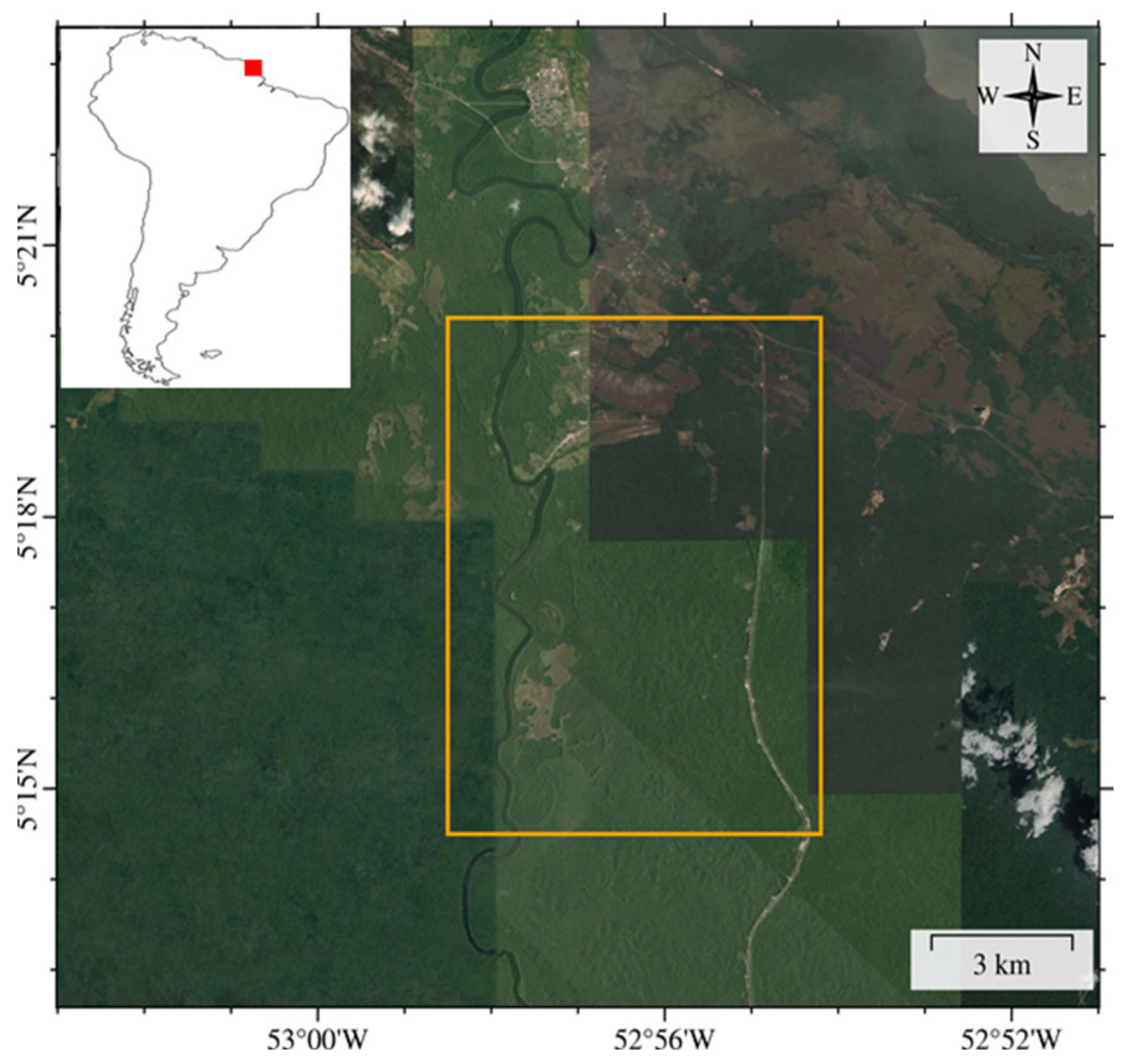
3. Study Area and Dataset

In order to verify the correctness and feasibility of the SKP-IMLE Pol-TomoSAR method, the P-band full polarimetric focused SAR images of the TropiSAR2009 project were used for the real data experiments. The study area was located in Paracou, French Guiana, and its geographic location is shown in Figure 1. This test area was a tropical forest containing many tree species. The forest height in the test area was roughly between 20 m and 45 m, and the altitude was between 5 m and 50 m.

The test area has six passes of fully polarimetric SAR images that were acquired by the ONERA SEFHI airborne system. The baseline length between adjacent orbits was about 15 m, and the incident angle variety was between 20 degrees and 60 degrees. The system parameters and baseline parameters of the SAR data in the test area are shown in

Table 2. System parameters and baseline configuration of TropiSAR2009 data set.

System Parameters		Baseline Configuration
		Number	Baseline Length
Wavelength	0.7542 m	0402	0 m
Center slant range	4905 m	0403	−14.4879 m
Center incident angle	35.0614°	0404	−30.1163 m
Range pixel spacing	1.000 m	0405	−43.8343 m
Azimuth pixel spacing	1.245 m	0406	−60.0632 m
Polarization	Fully polarized	0407	−74.9683 m

. In addition, the French Agricultural Research Center for International Development (CIRAD) enabled the light detection and ranging (LiDAR) data to cover a small part of the test area, which was used to verify the correctness and accuracy of the inversion results.

In order to evaluate the accuracy of the forest height and underlying topography retrieved by the proposed method, two test lines and two regions of interest (ROI) with different mean forest height were selected for inversion. The mean tree height of ROI1 was 28.9 m and the mean tree height of ROI2 was 25.6 m. The positions of the two ROI in the SAR images and the corresponding averaged LiDAR DTM and CHM are shown in Figure 2 and Figure 3.

4. Results

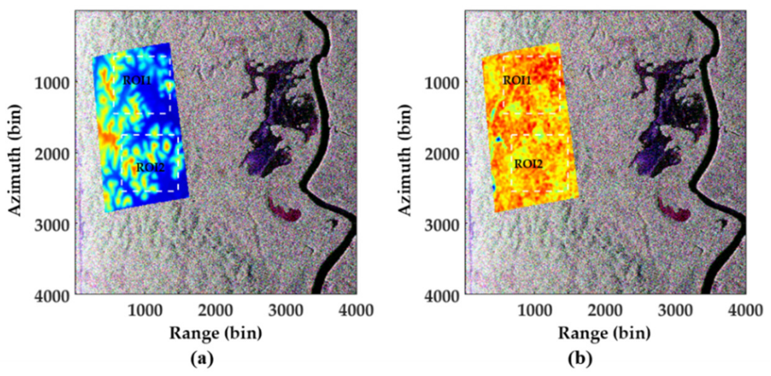
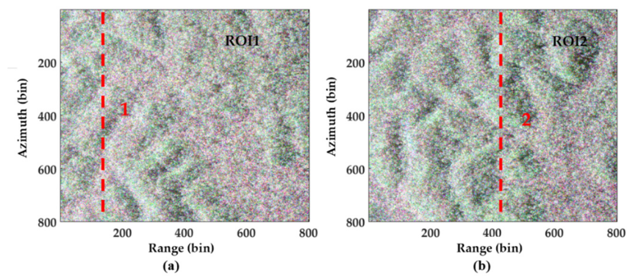
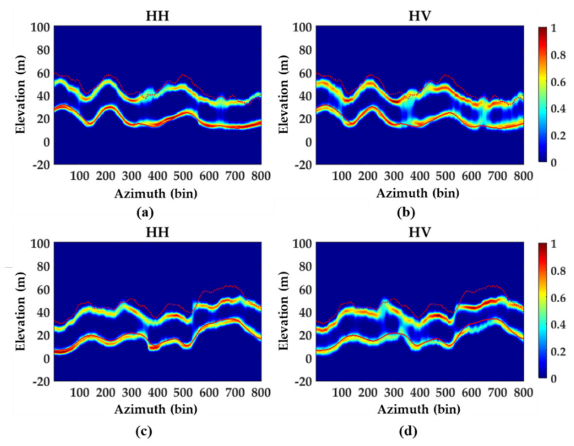
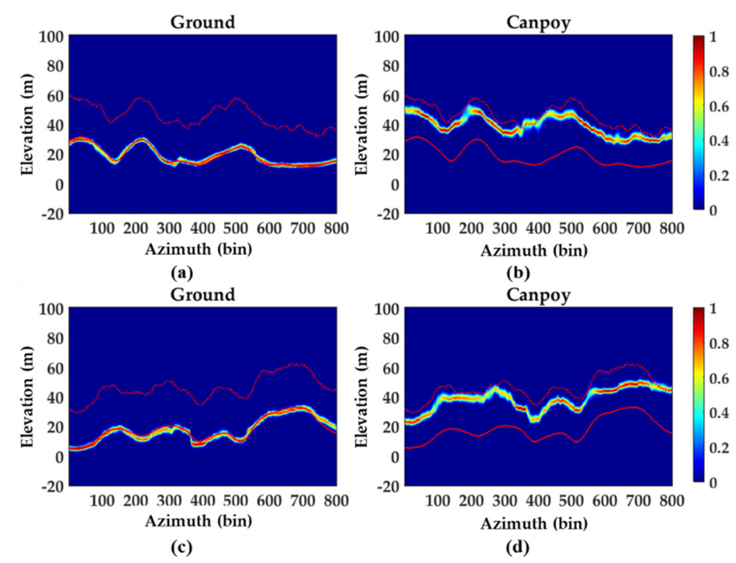
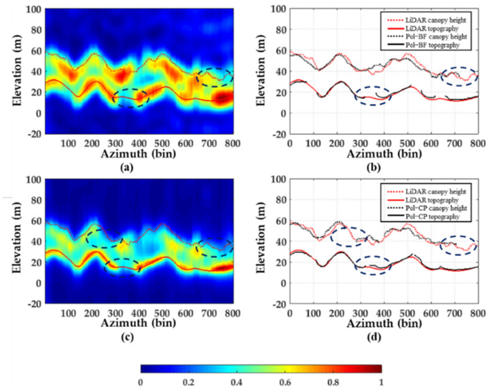
4.1. Tomograms of the Selected Azimuth Profiles

In order to verify the high resolution of the IMLE method in single-polarimetric TomoSAR and its ability to focus the canopy phase centers and the ground phase centers, two azimuth profiles (the red dashed lines in Figure 3) were selected for estimating the tomograms of HH channel and HV channel, respectively.

In the inversion process, the window size used to estimate the covariance matrix of multibaseline SAR data was 39 × 39 pixels, which roughly corresponds to the 50 m × 50 m in the ground range and azimuth plane. In order to keep the balance between inversion accuracy and calculation efficiency, the maximum number of iterations was set to 10.

Figure 4 shows the normalized tomograms of the two test lines at different locations estimated using the IMLE method. All the tomograms were clear and the phase centers of different scattering mechanisms were clearly distinguished. It can be seen from the tomograms that the scattering power of the HH polarimetric channel was mainly concentrated on the ground (as shown in Figure 4a,c), while the scattering power of the HV polarimetric channel was mainly concentrated on the canopy (as shown in Figure 4b,d). In addition, the tomograms of all polarimetric channels were in agreement with the LiDAR data.

The inversion results of two test lines at different positions also confirmed that the IMLE method had good reconstruction performance at both near slant-range and far slant-range locations. The continuous and highly focused phase centers of different scattering mechanisms were obtained from both polarimetric channels (see Figure 4). However, due to the influence of forest density, electromagnetic wave power, forest height, and other factors, there was no guarantee that vertical profile could generate two clear and separate peaks for all resolution cells.

In order to obtain more accurate inversion results of forest height and underlying topography, as well as to make the inversion strategy more stable, the SKP-IMLE Pol-TomoSAR estimator proposed in this paper could be used to estimate the tomograms of different scattering mechanisms for the two test lines.

Figure 5 shows that the SKP-IMLE Pol-TomoSAR method obtained more focused tomograms than the IMLE method for a single polarimetric channel. The tomograms of canopy scattering and ground scattering at two test lines were continuous, which was consistent with the LiDAR data. The phase centers of different scattering mechanisms were accurately located from the corresponding tomograms. Most importantly, the SKP-IMLE method ensured that we extracted the corresponding phase centers from the tomograms in all resolution cells.

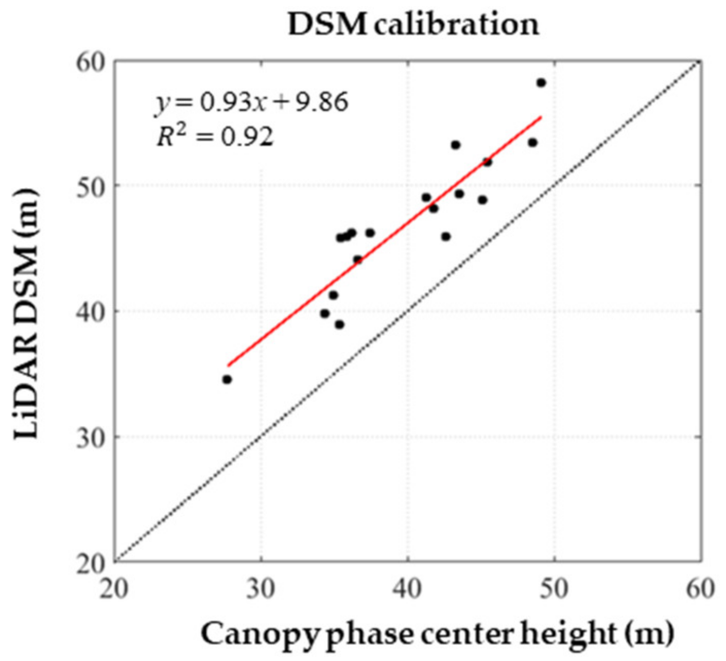
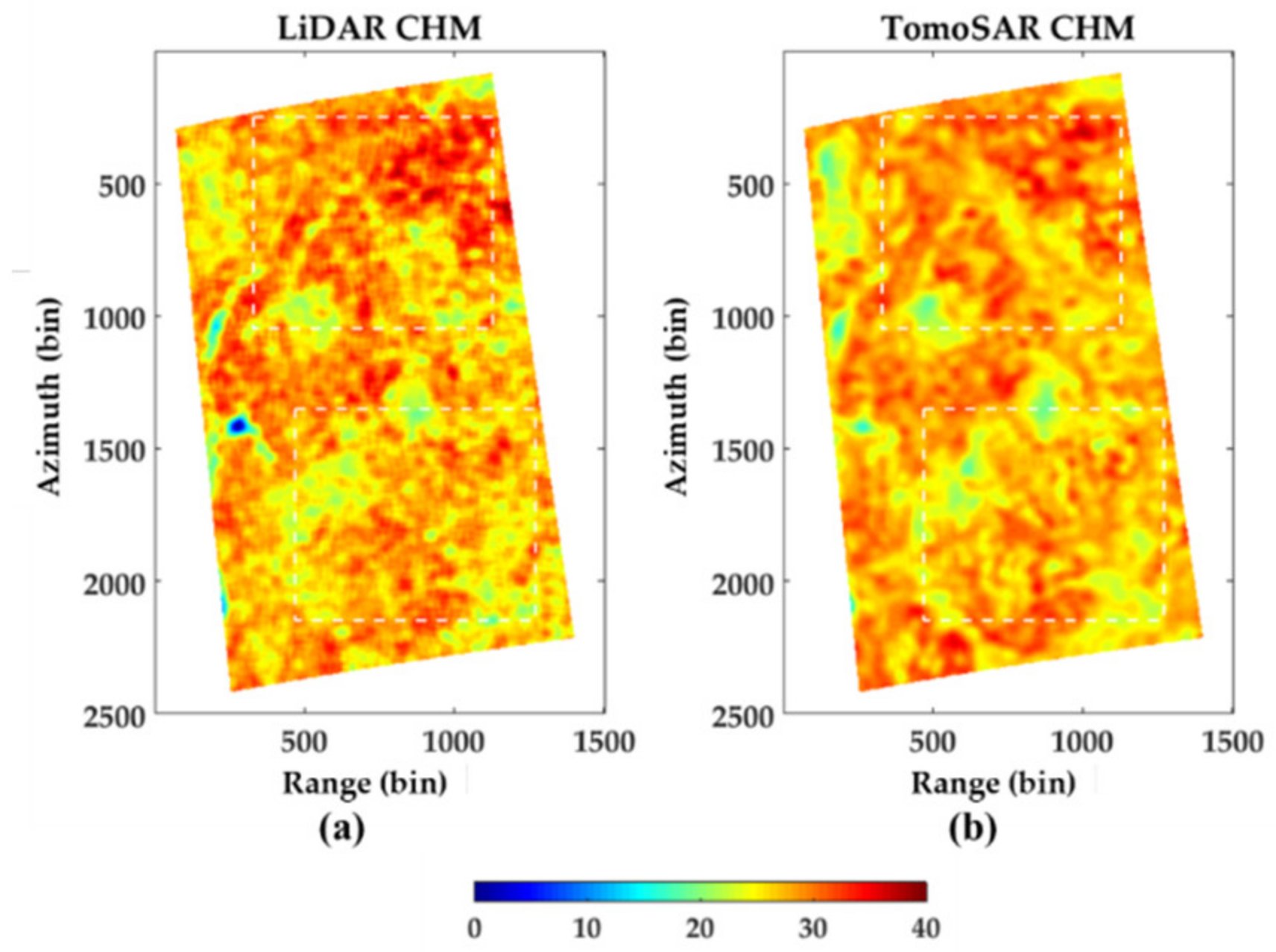
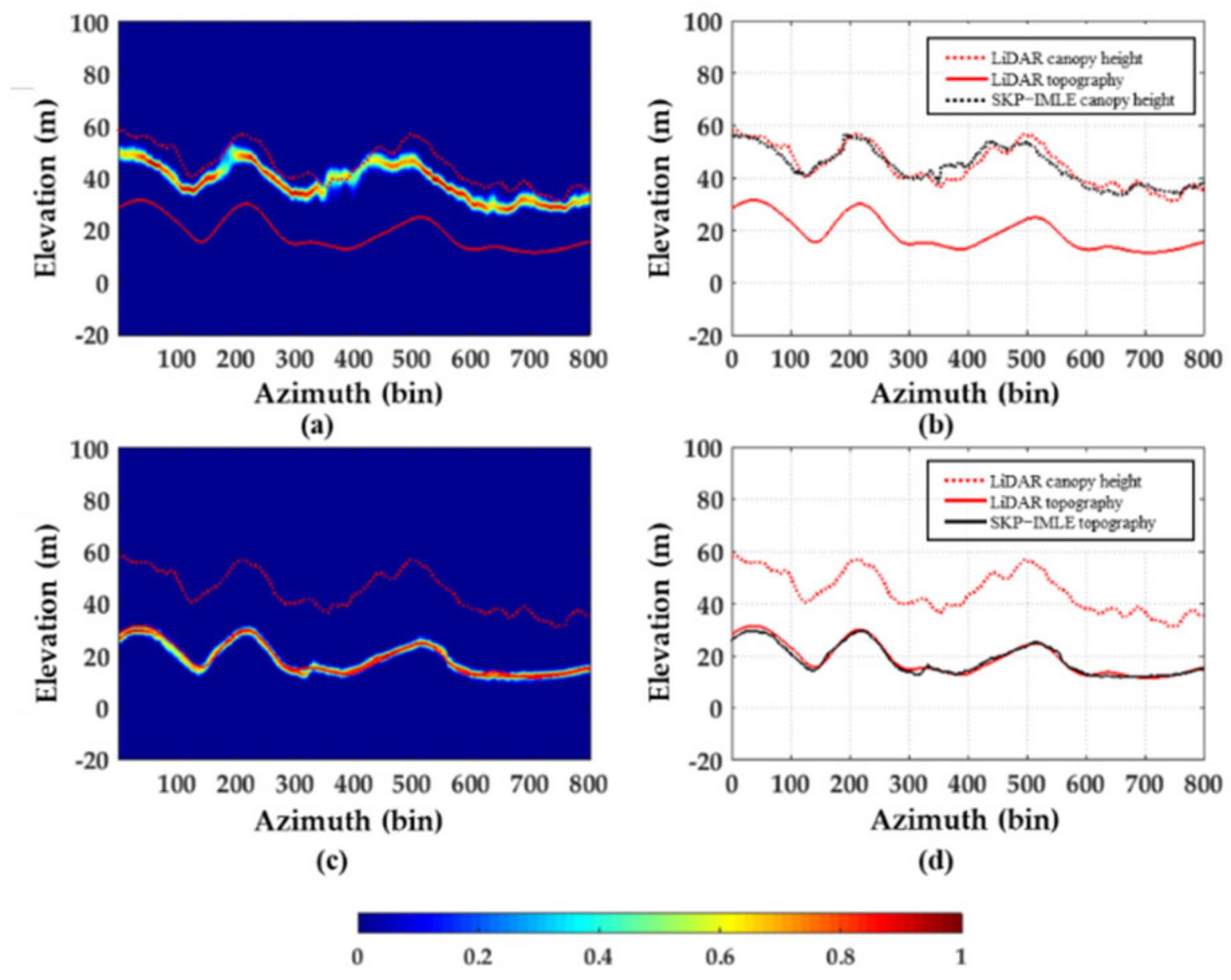
4.2. Forest Height and Underlying Topography Inversion

Based on the high-quality tomograms obtained using the SKP-IMLE method, the phase centers of different scattering mechanisms were extracted. Then, the underlying topography could be inverted based on the height values of the ground phase centers, and the forest height could be inverted based on the height values of the canopy phase centers. It should be noted that the locations of treetop were above the locations of the canopy phase centers (as shown in Figure 5b,d). The extracted canopy phase center positions still need to be corrected. For this purpose, 18 samples were selected in the test area, and the average height of the LiDAR-based digital surface model (DSM) in each sample was used to calibrate the phase center height according to (20). After that, the DSM was inverted via the SKP-IMLE method was obtained according to the calibration criterion (as shown in Figure 6). The terrain height was subtracted from the DSM to obtain the estimated value of the forest height.

Figure 7 and Figure 8 show the forest height and underlying topography retrieved via the SKP-IMLE Pol-TomoSAR method. The experimental results show that the SKP-IMLE method successfully reconstructed the underlying topography and forest height of the study area. Both the values of forest height and underlying terrain retrieved in the two ROIs were in good agreement with the LiDAR measurements.

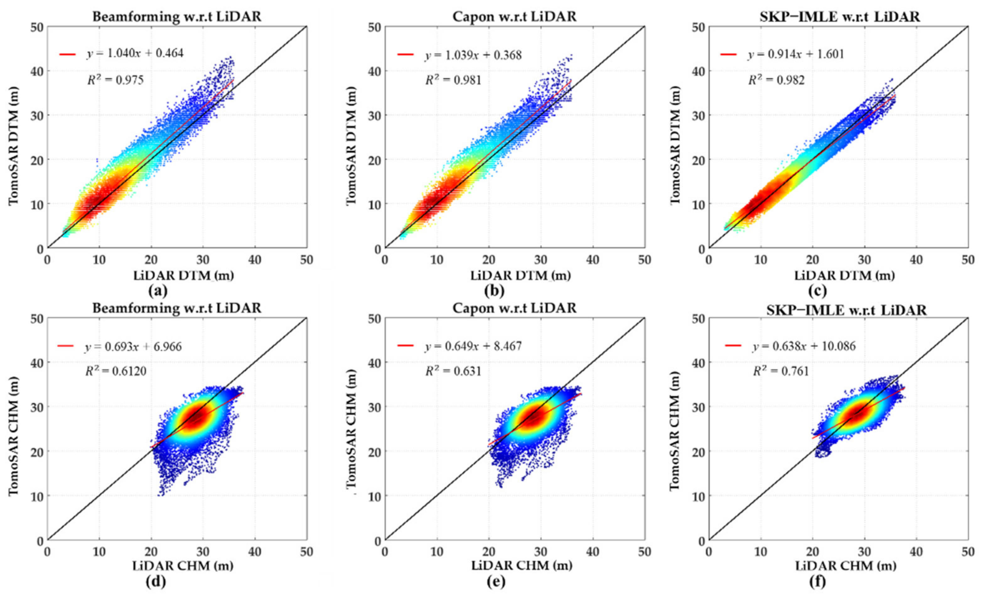
4.3. Comparison Experiments

In order to compare the reconstruction performance of the proposed method and the traditional Pol-TomoSAR methods (such as Pol-beamforming and Pol-Capon), the retrieved tomograms of test line1 were selected for analysis, and the forest height and underlying topography were extracted from the tomograms. The specific processes of the polarimetric Capon and beamforming methods were previously introduced in [24,25]. It should be noted that the window size used to estimate the covariance matrices in the beamforming method and Capon method was the same as that of the SKP-IMLE method.

Taking the tomograms of test line1 as an example (as shown in Figure 9a,c), SKP-IMLE obtained continuous and accurate phase centers. At the same time, the forest height and underlying topography retrieved from the tomograms were in agreement with the LiDAR measurements.

Although the Pol-beamforming method and the Pol-Capon method have the ability to distinguish scatterers with different scattering mechanisms, they still cannot achieve accurate positioning of the phase centers. In some resolution cells, only the phase centers of one scattering mechanism can be detected, and the inverted phase centers are not continuous (see the blue elliptical areas in Figure 10a,c). Therefore, the underlying topography and forest height information extracted by these two methods were not continuous (see the blue elliptical areas in Figure 10b,d).

Figure 11 and Figure 12 show the relationships between the inversion results and the LiDAR measurements. In addition, the root-mean-square error (RMSE) between the results and the LiDAR measurements is shown in

Table 3. Quantitative comparison of the employed methods with respect to LiDAR measurements.

		Pol-Beamforming	Pol-Capon	SKP-IMLE
ROI1	CHM (m)	3.390	3.076	1.997
	DTM (m)	2.014	1.769	1.489
ROI2	CHM (m)	5.871	4.750	1.765
	DTM (m)	3.076	2.429	1.786

.

Figure 11 shows the results of three TomoSAR methods in ROI1. At the same time, the correlation coefficients between the inversion results and the LiDAR measurements were also calculated. The experimental results show that the inversion results of SKP-IMLE were the most relevant to LiDAR measurements (as shown in Figure 11e,f), and had the highest inversion accuracy (as shown in Table 3).

The mean tree height in ROI2 is lower than that of RO11, and the canopy phase centers may be closer to the ground phase centers. Therefore, the inversion of forest height and underlying topography in ROI2 requires higher vertical resolution. The experimental results show that the SKP-IMLE method maintained a good performance in this area (as shown in Figure 12e,f). However, the reconstruction performances of the traditional methods were significantly reduced. In particular, the inversion result of forest height became very unreliable.

5. Discussion

In the experiment using TropiSAR2009 SAR data set, two different ROI and two different profiles were chosen to verify and analyze the proposed SKP-IMLE TomoSAR method. The experimental results showed that the new method obtained continuous tomograms of different scattering mechanisms in forest areas (as shown in Figure 5). Based on high-quality tomograms, accurate forest height and underlying topography could be retrieved (as shown in Table 3). The performance of the proposed method was also compared with other methods. We found that the main factor affecting the inversion accuracy is the resolution of the TomoSAR method. Due to the superior performance of SKP-IMLE, it obtained higher inversion accuracy in both ROI. In ROI1, the RMSE of the estimations from the SKP-IMLE method was 1.489 m for the underlying topography and 1.997 m for the forest height, which were both much less than the results of traditional spectral analysis methods. In ROI2, the inversion performances of the traditional methods were seriously degraded, but the SKP-IMLE method still obtained high-quality inversion results (as shown in Figure 12). In ROI2, the RMSE of the estimations from the SKP-IMLE method was 1.786 m for the underlying topography and 1.765 m for the forest height. Due to the limitation of vertical resolution, the traditional TomoSAR methods had low accuracy in the inversion of forest height and underlying topography. The underlying topography was obviously overestimated, while the forest height was obviously underestimated (as shown in Figure 11 and Figure 12). It was usually difficult to identify two separate phase centers in all pixels, resulting in large errors in the positioning of the phase centers.

Although the proposed method has many advantages, there are still some limitations in actual forest monitoring. The stability of the algorithm under different baseline configurations needs to be discussed because there are several matrix-vector operations, including matrix inversions. In addition, the algorithm needs to be optimized to improve its computational efficiency and improve its applicability in large-scale forest height inversion.

6. Conclusions

In this paper, we proposed a Pol-TomoSAR method based on SKP decomposition and maximum likelihood estimation. The new method was used in the inversion of forest height and underlying topography over a tropical forest, and reliable results were obtained. The performance of the proposed method was compared with two traditional TomoSAR methods. Through real data and comparative experiments, the following conclusions can be drawn:

(1)

The SKP-IMLE method has a high vertical resolution, so it can clearly distinguish the scatterers with different scattering mechanisms and achieve high focus of canopy scattering and ground scattering, which is very beneficial for forest height and underlying topography extraction. However, the traditional TomoSAR methods (such as beamforming and Capon) have limited resolution, and there is no guarantee that the vertical profile generates two clear and separate peaks for all resolution cells. These shortcomings make the extraction of forest height and underlying topography using traditional spectral analysis methods prone to errors.

(2)

The proposed SKP-IMLE method can obtain good forest height and underlying topography inversion results in tropical forests. With respect to LiDAR measurements, the SKP-IMLE method achieved high inversion accuracy in the two regions of interest.

In conclusion, the SKP-IMLE method has a high vertical resolution and can obtain reliable forest height and underlying topography inversion results even in dense tropical forest areas. Finally, further work will focus on using SKP-IMLE in SAR tomography with a small number of measurements. In addition, the proposed method will be used to estimate the height of boreal forests to test its applicability in different types of forests.

References

1. Colliander, A.; Narhi, T.; de Maagt, P. Modeling and Analysis of Polarimetric Synthetic Aperture Interferometric Radiometers Using Noise Waves. IEEE Trans. Geosci. Remote Sens. 2010, 48, 3560–3570. [Google Scholar] [CrossRef]
2. Lopez-Martinez, C.; Papathanassiou, K. Cancellation of Scattering Mechanisms in Polinsar: Application to Underlying Topography Estimation. IEEE Trans. Geosci. Remote Sens. 2013, 51, 953–965. [Google Scholar] [CrossRef]
3. Neumann, M.; Ferro-Famil, L.; Reigber, A. Estimation of Forest Structure; Ground; and Canopy Layer Characteristics from Multibaseline Polarimetric Interferometric Sar Data. IEEE Trans. Geosci. Remote Sens. 2010, 48, 1086–1104. [Google Scholar] [CrossRef] [Green Version]
4. Cloude, S.; Papathanassiou, K. Three-Stage Inversion Process for Polarimetric Sar Interferometry. IEE Proc.-Radar Sonar Navig. 2003, 150, 125–134. [Google Scholar] [CrossRef] [Green Version]
5. Papathanassiou, K.; Cloude, S. Single-Baseline Polarimetric Sar Interferometry. IEEE Trans. Geosci. Remote Sens. 2001, 39, 2352–2363. [Google Scholar] [CrossRef] [Green Version]
6. Reigber, A.; Moreira, A. First Demonstration of Airborne Sar Tomography Using Multibaseline L-Band Data. IEEE Trans. Geosci. Remote Sens. 2000, 38, 2142–2152. [Google Scholar] [CrossRef]
7. Cazcarra-Bes, V.; Tello-Alonso, M.; Fischer, R.; Heym, M.; Papathanassiou, K. Monitoring of Forest Structure Dynamics by Means of L-Band Sar Tomography. Remote Sens. 2017, 9, 1229. [Google Scholar] [CrossRef] [Green Version]
8. Minh, D.H.T.; Le Toan, T.; Rocca, F.; Tebaldini, S.; Villard, L.; Rejou-Mechain, M.; Phillips, O.L.; Feldpausch, T.R.; Dubois-Fernandez, P.; Scipal, K.; et al. Sar Tomography for the Retrieval of Forest Biomass and Height: Cross-Validation at Two Tropical Forest Sites in French Guiana. Remote Sens. Environ. 2016, 175, 138–147. [Google Scholar] [CrossRef] [Green Version]
9. Minh, D.H.T.; Tebaldini, S.; Rocca, F.; Le Toan, T.; Villard, L.; Dubois-Fernandez, P.C. Capabilities of Biomass Tomography for Investigating Tropical Forests. IEEE Trans. Geosci. Remote Sens. 2015, 53, 965–975. [Google Scholar] [CrossRef]
10. Minh, D.H.T.; Le Toan, T.; Rocca, F.; Tebaldini, S.; d’Alessandro, M.M.; Villard, L. Relating P-Band Synthetic Aperture Radar Tomography to Tropical Forest Biomass. IEEE Trans. Geosci. Remote Sens. 2014, 52, 967–979. [Google Scholar] [CrossRef]
11. Peng, X.; Li, X.; Wang, C.; Fu, H.; Du, Y. A Maximum Likelihood Based Nonparametric Iterative Adaptive Method of Synthetic Aperture Radar Tomography and Its Application for Estimating Underlying Topography and Forest Height. Sensors 2018, 18, 2459. [Google Scholar] [CrossRef] [Green Version]
12. Peng, X.; Li, X.; Wang, C.; Zhu, J.; Liang, L.; Fu, H.; Du, Y.; Yang, Z.; Xie, Q. Spice-Based Sar Tomography over Forest Areas Using a Small Number of P-Band Airborne F-Sar Images Characterized by Non-Uniformly Distributed Baselines. Remote Sens. 2019, 11, 975. [Google Scholar] [CrossRef] [Green Version]
13. Tebaldini, S. Single and Multipolarimetric Sar Tomography of Forested Areas: A Parametric Approach. IEEE Trans. Geosci. Remote Sens. 2010, 48, 2375–2387. [Google Scholar] [CrossRef]
14. Stoica, P.; Nehorai, A. MUSIC, maximum likelihood, and Cramer–Rao bound: Further results and comparisons. IEEE Trans. Acoust. Speech Signal Process. 1990, 38, 2140–2150. [Google Scholar] [CrossRef]
15. Lombardini, F.; Reigber, A. Adaptive Spectral Estimation for Multibaseline Sar Tomography with Airborne L-Band Data. Int. Geosci. Remote Sens. Symp. 2003, 3, 2014–2016. [Google Scholar]
16. Cazcarra-Bes, V.; Pardini, M.; Tello, M.; Papathanassiou, K. Comparison of Tomographic Sar Reflectivity Reconstruction Algorithms for Forest Applications at L-Band. IEEE Trans. Geosci. Remote Sens. 2020, 58, 147–164. [Google Scholar] [CrossRef]
17. Aguilera, E.; Nannini, M.; Reigber, A. Wavelet-Based Compressed Sensing for Sar Tomography of Forested Areas. IEEE Trans. Geosci. Remote Sens. 2013, 51, 5283–5295. [Google Scholar] [CrossRef] [Green Version]
18. Donoho, D.L. Compressed Sensing. IEEE Trans. Inf. Theory 2006, 52, 1289–1306. [Google Scholar] [CrossRef]
19. Li, X.; Liang, L.; Guo, H.; Huang, Y. Compressive Sensing for Multibaseline Polarimetric Sar Tomography of Forested Areas. IEEE Trans. Geosci. Remote Sens. 2016, 54, 153–166. [Google Scholar] [CrossRef]
20. Zhu, X.X.; Bamler, R. Very High Resolution Spaceborne Sar Tomography in Urban Environment. IEEE Trans. Geosci. Remote Sens. 2010, 48, 4296–4308. [Google Scholar] [CrossRef] [Green Version]
21. Zhu, X.X.; Bamler, R. Super-Resolution Power and Robustness of Compressive Sensing for Spectral Estimation with Application to Spaceborne Tomographic SAR. IEEE Trans. Geosci. Sens. 2012, 50, 247–258. [Google Scholar] [CrossRef]
22. Martín del Campo, G.D.; Nannini, M.; Reigber, A. Statistical Regularization for Enhanced TomoSAR Imaging. IEEE J. Sel. Top. Appl. Earth Observ. Remote Sens. 2020, 13, 1567–1589. [Google Scholar] [CrossRef]
23. Martín del Campo, G.D.; Nannini, M.; Reigber, A. Towards feature enhanced SAR tomography: A maximum-likelihood inspired approach. IEEE Geosci. Remote Sens. Lett. 2018, 15, 1730–1734. [Google Scholar] [CrossRef]
24. Ferro-Famil, L.; Huang, Y.; Tebaldini, S. Polarimetric Characterization of 3-D Scenes using High-resolution and Full-Rank Polarimetric Tomographic SAR Focusing. In Proceedings of the 2016 IEEE International Geoscience and Remote Sensing Symposium (IGARSS), Beijing, China, 10–15 July 2016. [Google Scholar]
25. Huang, Y.; Ferro-Famil, L.; Reigber, A. Under-Foliage Object Imaging Using SAR Tomography and Polarimetric Spectral Estimators. IEEE Trans. Geosci. Sens. 2012, 50, 2213–2225. [Google Scholar] [CrossRef] [Green Version]
26. Aguilera, E.; Nannini, M.; Reigber, A. A Data Adaptive Compressed Sensing Approach to Polarimetric SAR Tomography. In Proceedings of the 2012 IEEE International Geoscience and Remote Sensing Symposium, Munich, Germany, 22–27 July 2012. [Google Scholar]
27. Huang, Y.; Levy-Vehel, J.; Ferro-Famil, L.; Reigber, A. Three-Dimensional Imaging of Objects Concealed Below a Forest Canopy Using Sar Tomography at L-Band and Wavelet-Based Sparse Estimation. IEEE Geosci. Remote Sens. Lett. 2017, 14, 1454–1458. [Google Scholar] [CrossRef]
28. Pardini, M.; Papathanassiou, K. On the Estimation of Ground and Volume Polarimetric Covariances in Forest Scenarios with SAR Tomography. IEEE Geosci. Remote Sens. Lett. 2017, 14, 1860–1864. [Google Scholar] [CrossRef] [Green Version]
29. Tebaldini, S. Algebraic Synthesis of Forest Scenarios from Multibaseline Polinsar Data. IEEE Trans. Geosci. Remote Sens. 2009, 47, 4132–4142. [Google Scholar] [CrossRef]
30. Tebaldini, S.; Rocca, F. Multibaseline Polarimetric Sar Tomography of a Boreal Forest at P- and L-Bands. IEEE Trans. Geosci. Remote Sens. 2012, 50, 232–246. [Google Scholar] [CrossRef]
31. Aghababaee, H.; Sahebi, M.R. Model-Based Target Scattering Decomposition of Polarimetric SAR Tomography. IEEE Trans. Geosci. Sens. 2018, 56, 972–983. [Google Scholar] [CrossRef]
32. Tebaldini, S.; Rocca, F. On the Impact of Propagation Disturbances on SAR Tomography: Analysis and Compensation. In Proceedings of the IEEE Radar Conference, Pasadena, CA, USA, 4–8 May 2009; pp. 1–6. [Google Scholar]
33. Shkvarko, Y.V. Unifying Regularization and Bayesian Estimation Methods for Enhanced Imaging with Remotely Sensed Data —Part 1: Theory. IEEE Trans. Geosci. Remote Sens. 2004, 42, 923–931. [Google Scholar] [CrossRef]
34. Shkvarko, Y.V. Unifying Regularization and Bayesian Estimation Methods for Enhanced Imaging with Remotely Sensed Data —Part 2: Implementation and Performance Issues. IEEE Trans. Geosci. Remote Sens. 2004, 42, 932–940. [Google Scholar] [CrossRef]
Figure 1. The geographic location of the study area. The yellow rectangle represents the footprint of the dataset.
Forests 12 00444 g001
Figure 2. The LiDAR DTM and CHM in the Pauli RGB SAR images: (a) LiDAR DTM; (b) LiDAR CHM. The white dotted areas are two regions of interest (ROI).
Forests 12 00444 g002
Figure 3. The two test lines in the Pauli RGB SAR images of ROI1 and ROI2: (a) test line1 in ROI1; (b) test line2 in ROI2.
Forests 12 00444 g003
Figure 4. The normalized tomograms of two test lines estimated by the IMLE method for two different polarimetric channels: (a) HH channel tomogram of test line1; (b) HV channel tomogram of test line1; (c) HH channel tomogram of test line2; (d) HV channel tomogram of test line2. The red dotted and solid lines represent DTM + CHM and DTM, respectively.
Forests 12 00444 g004
Figure 5. The normalized tomograms of two test lines estimated by the SKP-IMLE method for two different scattering mechanisms: (a) ground scattering of test line1; (b) canopy scattering of testline1; (c) ground scattering of test line2; (d) canopy scattering of testline2. The red dotted and solid lines represent DTM+CHM and DTM, respectively.
Forests 12 00444 g005
Figure 6. Correlation analysis between the LiDAR DSM and the canopy phase center height estimated by the SKP-IMLE method.
Forests 12 00444 g006
Figure 7. The DTM estimated by the SKP-IMLE method: (a) LiDAR DTM; (b) TomoSAR DTM. The white dotted areas are the estimated DTM and LiDAR DTM of the two regions of interest (ROI).
Forests 12 00444 g007
Figure 8. The CHM estimated by the SKP-IMLE method: (a) LiDAR CHM; (b) TomoSAR CHM. The white dotted areas are the estimated CHM and LiDAR CHM of the two ROI.
Forests 12 00444 g008
Figure 9. The normalized tomograms of test line1 estimated by SKP-IMLE method and the forest height and underlying topography extracted from the tomograms: (a) tomogram of ground scattering; (b) estimated forest height of test line1; (c) tomogram of ground scattering; (d) estimated underlying topography of test line1.
Forests 12 00444 g009
Figure 10. The normalized tomograms of test line1 estimated by traditional PolTomoSAR methods and the forest height and underlying topography extracted from the tomograms: (a) tomogram estimated using Pol-beamforming method; (b) forest height and underlying topography of test line1 estimated using Pol-beamforming method; (c) tomogram estimated using Pol-Capon method; (d) forest height and underlying topography of test line1 estimated using Pol-Capon method.
Forests 12 00444 g010
Figure 11. The relationships between the LiDAR and TomoSAR heights in ROI1: (a) LiDAR-based DTM and underlying topography by the Pol-beamforming method; (b) LiDAR-based DTM and underlying topography by the Pol-Capon method; (c) LiDAR-based DTM and underlying topography by the SKP-IMLE method; (d) LiDAR-based CHM and forest height by the Pol-beamforming method; (e) LiDAR-based CHM and forest height by the Pol-Capon method; (f) LiDAR-based CHM and forest height by the SKP-IMLE method.
Forests 12 00444 g011
Figure 12. The relationships between the LiDAR and TomoSAR heights in ROI2: (a) LiDAR-based DTM and underlying topography by the Pol-beamforming method; (b) LiDAR-based DTM and underlying topography by the Pol-Capon method; (c) LiDAR-based DTM and underlying topography by the SKP-IMLE method; (d) LiDAR-based CHM and forest height by the Pol-beamforming method; (e) LiDAR-based CHM and forest height by the Pol-Capon method; (f) LiDAR-based CHM and forest height by the SKP-IMLE method.
Forests 12 00444 g012