Abstract
From supporting wood production to mitigating climate change, forest ecosystem services are crucial to the well-being of humans. Understanding the mechanisms that drive forest dynamics can help us infer how to maintain forest ecosystem services and how to improve predictions of forest dynamics under climate change. Despite the growing number of studies exploring above ground biomass (AGB) dynamics, questions of dynamics in biodiversity and in number of individuals still remain unclear. Here, we first explored the patterns of community dynamics in different aspects (i.e., AGB, density and biodiversity) based on short-term (five years) data from a 25-ha permanent plot in a subtropical forest in central China. Second, we examined the relationships between community dynamics and biodiversity and functional traits. Third, we identified the key factors affecting different aspects of community dynamics and quantified their relative contributions. We found that in the short term (five years), net above ground biomass change (ΔAGB) and biodiversity increased, while the number of individuals decreased. Resource-conservation traits enhanced the ΔAGB and reduced the loss in individuals, while the resource-acquisition traits had the opposite effect. Furthermore, the community structure contributed the most to ΔAGB; topographic variables and soil nutrients contributed the most to the number of individuals; demographic process contributed the most to biodiversity. Our results indicate that biotic factors mostly affected the community dynamics of ΔAGB and biodiversity, while the number of individuals was mainly shaped by abiotic factors. Our work highlighted that the factors influencing different aspects of community dynamics vary. Therefore, forest management practices should be formulated according to a specific protective purpose.
1. Introduction
The forest ecosystem, accounting for over 70% terrestrial biomass, supports high levels of global terrestrial biodiversity [1,2,3]. This makes forests crucial to the existence and sustainable development of human society, from supporting wood production to sequestering carbon and to mitigating climate change [4,5]. However, anthropogenic activities and dramatic climate change have disrupted the balance of forest ecosystems [6]. Hence, in order to maintain steady ecosystem services and functions, it is necessary and urgent for ecologists to understand the mechanisms underlying forest community dynamics [7]. The dynamics of above ground biomass (AGB, an important ecosystem function) in forests have been well-studied [8,9,10,11], thus confirming the effect of both biotic factors (e.g., biodiversity, functional traits) and abiotic factors (e.g., topographic variables, soil nutrients) on AGB dynamics. However, these studies only investigated one aspect of forest dynamics, so do not provide enough information for readers to understand how forest ecosystem services and functions will respond to climate change altogether. In other words, other aspects of community dynamics such as the changes in diversity and in number of individuals, are still poorly understood, and so are the underlying mechanisms that drive these different aspects of forest dynamics [12,13,14]. For example, one experiment in a Minnesota grassland showed that although the above ground biomass increased significantly after nitrogen addition, diversity decreased, and thus reduced the stability in grassland ecosystem function [15].
The effects of biodiversity on forest community dynamics, especially on the AGB dynamics, have achieved sufficient research attention in many forest types including boreal [14,16], temperate [11,17,18], and tropical forests [8,10]. Most of these studies have confirmed the positive effect of biodiversity and have posited two hypotheses to explain the underlying mechanisms. The first hypothesis of selection effect states that a hyper-diverse community has a greater chance of containing more productive species, which thus enhances AGB [19]; the second hypothesis of complementarity effect states that facilitation and niche differentiation augment ecosystem function due to higher resource use efficiency [20]. However, some authors have reported that a positive effect of biodiversity was only observed in species-poor communities [16,21]. Therefore, whether the effect of biodiversity is efficient for net above ground change and for other aspects of community dynamics in species-rich subtropical forests needs to be studied. The role of functional traits on community dynamics has also been considered [8,16,17]. For instance, the mass ratio hypothesis states that ecosystem functions are mainly determined by the functional traits of dominant plants in the community [22]. The communities with fast-growing acquisitive traits are prone to higher productivity, whereas the communities with slow-growing conservative traits are prone to stability and lower productivity [16,17]. However, previous studies have reported that the mass ratio hypothesis is contingent on environmental conditions, for instance, one study in tropical dry forests did not support this hypothesis [9].
Structural forest community characteristics (e.g., density, the ratio of large or small trees) are regarded as another group of important biotic factors for community dynamics [23,24]. The vegetation hypothesis predicts that ecosystem function is primarily driven by vegetation quantity rather than vegetation quality [25]. For example, a higher tree density can increase AGB because of higher canopy packing and leaf area index [5,26]. Large trees are also regarded as critical for community dynamics due to their resistance to external disturbance and advantages in acquiring light to aid their growth [11,27]. For instance, Yuan et al. [11] reported that a few large trees drive AGB stock and the dynamics of temperate forests in northeast China, more than even plant diversity and composition. Finally, small trees are thought to have less importance on AGB dynamics than large trees [28] because their lower competitive ability and stress-tolerance leads to larger fluctuations in individuals.
Moreover, demographic processes (e.g., recruitment and mortality) are crucial for predicting community species composition, and therefore for directly regulating community dynamics [14,17,29]. Mortality, which is mostly determined by competition and environmental conditions [30], was found to be a major factor leading to net AGB change in forests [10,17]. In contrast, recruitment is thought to be associated with species turnover and community functional composition shift as well as directly related to the change in number of individuals [31,32], though it contributes little to AGB dynamics [33].
In addition to the biotic factors above-mentioned, abiotic factors (i.e., topographic variables and soil nutrients) also play a key role in forest dynamics [34,35]. Topographic variables such as elevation, convexity, slope, and aspect affect community biomass and species composition and also redistribute heat and moisture at a local scale [36]. For example, elevation and convexity can modify microclimate by affecting conditions such as soil humidity and temperature. Aspect is directly related to light intensity, and slope is closely related to the site condition of trees [37]. Soil nutrients are also critical in regulating community dynamics through the effect they have on plant functional traits, community diversity and even interspecific competition [38]. For example, soil nutrients such as soil phosphorus content mainly drive the biomass dynamics in Amazonian forests [39], though the neutral effect was also observed in this area [9]. Thus, how abiotic factors affect community dynamics in subtropical forests need clarity.
In this study, we analyzed a large dataset from two censuses five years apart in a 25-ha subtropical forest, aiming to explore the relationships between community dynamics and biotic (i.e., biodiversity, functional traits, forest structure, demographic process) and abiotic factors (i.e., topographic variables and soil nutrients). We addressed the following three major questions: (1) What is the pattern of community dynamics in this subtropical forest, and is there a significant difference among different topographic conditions? (2) How do biodiversity and functional traits affect the community dynamics in species-rich subtropical forests, and does the effect differ among different aspects of community dynamics? and (3) What are the key influencing factors on the three aspects of community dynamics, and what are their relative contributions?
2. Materials and Methods
2.1. Study Site and Data Collection
The study was conducted in the Badagongshan (BDGS) National Nature Reserve in Hunan Province, China (29°39′18″–29°49′48″ N, 110°41′45″–110°09′50″ E). This National Nature Reserve was established in 1986 to prevent anthropogenic disturbance. The area is characterized by a subtropical humid monsoon climate with a seasonal annual rainfall pattern. Most rainfall occurs between March and October. Annual mean temperature in the region is 11.5 °C, ranging from 0.1 °C in January to 23.3 °C in July. Mean annual precipitation is 2105 mm with an average of 176 rain days per year. The study region is characterized by rolling mountainous terrain, with elevation ranging from 1354.7 m to 1455.9 m above sea level (a.s.l.). The soil in the region is typical paleudalfs soil. Forest covers 93.4% of the reserve area [37].
The 25 ha (500 m × 500 m) forest plot was established in 2011 and can be divided into 625 cells 20 m × 20 m contiguous subplots. All the individuals of woody plant with a diameter at breast height (DBH) ≥ 1 cm in the plot had their DBH measured, mapped, identified to species and tagged. In the first census, the plot contained more than 186,000 stems of 232 species (93 evergreen and 139 deciduous), representing 53 families and 114 genera [40]. The forest is dominated by Cyclobalanopsis multinervis and Fagus lucida. Other important species include Cyclobalanopsis gracilis, Quercus serrata var. brevipetiolata, Schima parviflora, Carpinus fargesii, Sassafras tzumu, Litsea elongate, and Rhododendron stamineum. The second census was conducted in 2016, and no disturbances occurred in our plot during these five years. All trees were remeasured. The recruits that had grown into the 1 cm size class were measured, mapped, identified to species and tagged, and information on newly dead individuals was recorded.
2.2. Metrics of Community Dynamics
We calculated the change of AGB (ΔAGB), the change rate of individuals (CRI), and the change in Shannon index (ΔS) in each subplot over the 5-year period to reflect the community dynamics. The AGB was calculated using a published above ground biomass model that was fitted effectively in this research area [37]. The ΔAGB, CRI, and ΔS were calculated as follows:
where AGB16 and AGB11 are the AGB of living trees in each 20 m × 20 m subplot in 2016 and 2011, respectively. N16 and N11 are the numbers of living individuals in each subplot in 2016 and 2011, respectively. S16 and S11 are the Shannon indexes of each subplot in 2011 and 2016, respectively (Supplementary Materials, Table S1).
2.3. Biotic Factors
2.3.1. Functional Traits and Biodiversity
To explore the relationships between community dynamics and biodiversity and with functional traits, we collected functional trait data for most species in the forest dynamics plot during the growing season (June–mid September) from 2012 to 2015. We sampled 10 individuals from common species (129). For rare species (33), which we defined as species having less than one individual per ha, we selected 3–5 individuals to sample. For each individual, we collected 10–20 healthy and mature leaves that were exposed to the sun. In all, we sampled 910 individuals, which included 64 evergreen species and 98 deciduous species. The species sampled (162 species), whose number was over 99% of total number of individuals, can reflect the major information about functional traits in our plot. For each sample, we measured eight plant functional traits including leaf area (LA, cm2), leaf thickness (LT, mm/m), specific leaf area (SLA, cm2/g), leaf carbon content (LCC, g/kg), leaf nitrogen content (LNC, g/kg), leaf phosphorus content (LPC, g/kg), leaf C/N ratio (LCN), and leaf dry matter content (LDMC, g). These traits have been found to be closely linked to community dynamics [41,42]. LT and LA were measured by Vernier calipers Deli DL3944 (Deli Inc., Ningbo, Zhejiang, China) and Canon CanoScan LiDE 110 portable electronic scanner (Canon Inc., Beijing, China), respectively. LMDC was calculated as the dry mass of a leaf divided by its saturated fresh weight. The LCC and LNC were determined using stable isotope mass spectrometry, and the LPC was determined using the molybdenum antimony resistance spectrophotometric method [43]. Then, we calculated the leaf C/N ratio (LCN) and specific leaf area (SLA) based on the measured traits. Next, we calculated the mean value of each trait at the species-level for use in the subsequent analysis. In addition, following the leaf economics spectrum [44], we divided the above-mentioned eight functional traits into two categories, namely resource-acquisition traits (i.e., SLA, LA, LNC, and LPC) and resource-conservation traits (i.e., LDMC, LT, LCC, and LCN).
To test the mass ratio hypothesis, we calculated the community-weighted means trait (CWM), which was weighted by the relative abundance of each species within a subplot. Then, we used principal component analysis to obtain the major information of the eight CWM traits. The first three axes (CWMPC1, CWMPC2, and CWMPC3) explained 82.55% of the total variation in the CWM factors. LDMC, LT, LCC, and LCN correlated negatively with CWMPC1, while SLA, LA, LNC, and LPC correlated positively with CWMPC1 (Table S2). CWM trait calculations and principal component analysis were carried out using the packages “FD” [45] and “vegan” [46] of R statistical language [47].
In this study, we explored the effects of species diversity (not for ΔS) and functional diversity on community dynamics. Species diversity was defined as the number of species in each subplot (species richness, SR). We used Rao’s quadratic entropy (Rao Q) to represent the functional diversity of each subplot using the functional traits described above. Rao Q is widely used in functional diversity studies, and accounts for both the pairwise functional distance between species and the relative abundances of each species [48]. The functional diversity calculation was performed in R package “FD” [45].
2.3.2. Community Structure and Demographic Process
Community structural attributes include community density and the proportion of large trees and of small trees within each subplot (Table S1). Community density was defined as the number of living trees within each subplot in 2011. Here, we defined a large tree as the approximately top 1% of widest trees by DBH, as in a previous study [11]. Therefore, trees with DBH > 30 cm were regarded as large trees in this study, and their number accounted for 1.16% of all individuals in our plot. In contrast, trees with DBH < 3 cm were regarded as small trees due to their vulnerability and lower capacity for competition. Small trees accounted for 53.81% of all individuals in our plot.
We used the recruitment and mortality of individuals within each subplot to reflect the community demographic process. Recruitment and mortality were calculated as the number of new recruits and dead individuals (DBH > 1 cm) within each subplot in 2016 divided by the total number of living trees in each subplot in 2011, respectively.
2.4. Abiotic Factors
2.4.1. Topographic Variables
Topographic variables included elevation, slope, aspect, and convexity. All variables were calculated in each subplot. Elevation was defined as the mean elevation of the four corners. Slope was calculated as the average angular deviation from horizontal of each of the four triangular planes formed by connecting three of the four corners. Aspect was the direction at which a slope faces, and the cosine of this variable was used to linearize the data. Convexity was the mean difference between the elevation of the focal subplot and the elevation of the eight adjacent subplots. For edge subplots, convexity was the elevation of the center point minus the mean of the four corners. The measurement of topographic variables followed the method described in Xu et al. [37]. In order to explore the difference in the pattern of subtropical forest community dynamics among different topographic conditions, we used multivariate tree regression (MRT) to divide the plot into three topographic sites, namely ridge (elevation ≥ 1438 m), slope (elevation < 1438 m and convexity ≥ −2.62), and valley (elevation < 1438 m and convexity ≤ −2.62) [49].
2.4.2. Soil Nutrients
To obtain the soil samples, we divided the main part of the plot (480 m × 480 m) into 30 m × 30 m grids [50], and the remaining part into 32 cells 20 m × 30 m grids and a 20 m × 20 m grid. We sampled the soil at the intersections of grid lines. Then, we randomly selected two additional points, each at a distance of 2 m, 5 m, and 15 m from the intersections. A total of 972 soil samples were taken from the plot [50]. The detailed soil sampling design is explained in Li et al. (2017). Soils were sampled from both the top (0–10 cm) and bottom (10–30 cm) soil layers. Soil pH, bulk density (BD, g/cm3), C density (CD), and soil temperature (T) were measured in the top soil layers. Soil total carbon (SC, %) and nitrogen (SN, %), phosphorus (P, mg/kg), and δ13C (C13) isotope were measured in both soil layers. The detailed measurement of soil nutrients can be found in Li et al. [50]. We then obtained soil nutrient parameters for each subplot by Ordinary Kriging using software Surfer version 16. To obtain the soil nutrient data for further analysis, we used principal component analysis. The first three axes explained 58.60% of total variation in the soil nutrients. The soil nitrogen and carbon in the upper soil layer correlated positively with SoilPC1; soil bulk density correlated positively with SoilPC2 (Table S3).
2.5. Statistical Analysis
To understand the short-term (five years) patterns of community dynamics in a subtropical forest, we first used Tukey’s test with a one-way analysis of variance (ANOVA) to test the differences in ΔAGB, CRI, and ΔS among the three topographic conditions (ridge, slope, and valley). To understand the effect of biodiversity (species richness, functional diversity) on community dynamics and to validate the mass ratio hypothesis, we used a linear regression model to analyze the bivariate relationship between community dynamics and biodiversity and functional traits.
In order to identify the key factors and their relative contribution to community dynamics, we used structural equation modeling (SEM). Before conducting this analysis, we used ordinary least squares (OLS) multiple regression to filter out the less important factors. All biotic (i.e., biodiversity, CWM traits, community structural attribution, and demographic process) and abiotic factors (i.e., topographic variables and soil nutrients) were standardized (Z-Score) and then included in the full model to explore their effects on ΔAGB. For ΔS, we did not include SR. Next, recruitment and mortality were excluded in the full model to explore their effects on the CRI, because CRI is an aggregate variable based on recruitment and mortality. To eliminate multicollinearity, we filtered out variables with variance inflation factor (VIF) > 5 in the multiple regression model [51]. To find the best model, we used the “MuMIn” [52] package in R, and selected the model with the lowest corrected Akaike information criterion (AIC) and number of predictors, and the highest adjusted R squared [5]. The final model for community dynamics can be found in Table 1. We then used the key factors included in the best model to explore their direct and indirect effects on community dynamics and their relative contribution by using the SEM model. The SEM was performed in the “lavaan” package [53] and was evaluated for goodness-of-fit using Bentler’s Comparative Fit Index (CFI > 0.90), standardized root mean square residual (SRMR ≤ 0.05), and a Chi-square (χ2) test (p-value > 0.05) [54]. All analyses above-mentioned were performed in software R version 3.6.0 [47].

Table 1.
The best multitude regression model for community dynamics.
3. Results
3.1. Patterns of Community Dynamics in a Subtropical Forest
The AGB and Shannon indexes increased from 2011 to 2016, with mean changes of 0.923 ± 0.026 Mg and 0.015 ± 0.001 at the subplot-level, respectively. The change rate of individuals (CRI) showed a decrease in the number of individuals from 2011 to 2016, with a mean value of −5.040 ± 0.232% at the subplot-level (Table 2). Specifically, the ΔAGB was highest on the ridge (1.070 ± 0.041 Mg), followed by the slope (0.948 ± 0.038 Mg) and valley (0.680 ± 0.055 Mg). The CRI was lowest in the valley (−6.972 ± 0.486%), followed by the slope (−5.206 ± 0.350%) and ridge (−3.365 ± 0.369%). The ΔS did not differ significantly among the three topographic conditions (Table 2).
Table 2.
The patterns of dynamics for different topographic conditions at the subplot (20 m × 20 m).
3.2. Relationship between Community Dynamics and Biodiversity and Functional Traits
Species richness (SR) positively influenced ΔAGB (p < 0.001), while functional diversity (Rao Q) negatively influenced ΔAGB (p < 0.001). In addition, Rao Q was significantly and negatively correlated with CRI (Table 3).
Table 3.
Bivariate relationships between community dynamics and functional traits and biodiversity.
Resource-acquisition traits (i.e., SLA, LA, LNC, and LPC) had significant and negative influences on both ΔAGB and CRI (Table 3). However, only LA of the resource-acquisition traits had a positive influence on ΔS (p = 0.007). All resource-conservation traits, except for LDMC, had significant and negative influences on both ΔAGB and CRI, while no resource-conservation traits influenced ΔS (Table 3).
3.3. The Relative Contribution of Influencing Factors on Community Dynamics
The SEM model (CFI = 1, SRMR = 0.001, χ2 = 0.01, p = 0.92) for ΔAGB showed that net above ground biomass change was directly affected by community density (β = 0.38), mortality (β = −0.27), and number of large trees (β = 0.21). Community density also indirectly enhanced the ΔAGB via mortality. Large trees also had indirect positive and negative effects on ΔAGB via community density and mortality, respectively (Figure 1). Community structure (70.59%, small trees (3.92%), large trees (19.61%), and density (47.06%)) contributed the most to ΔAGB, followed by demographic process (mortality, 26.47%), and topographic variable (cos(aspect), 2.94%, Figure 2).
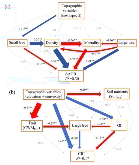
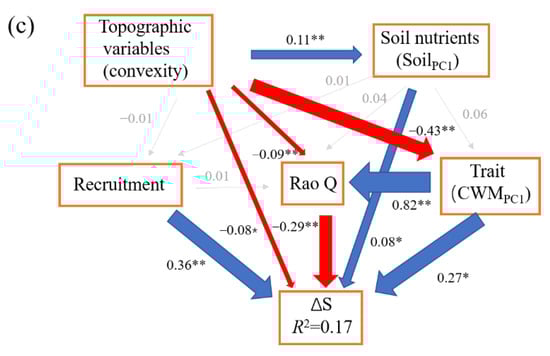
Figure 1.
The structural equation models for the change of above ground biomass (ΔAGB) (a), the change rate of individuals (CRI) (b), and the change in Shannon index (ΔS) (c). The blue lines represent the significant and positive paths (* p < 0.05; ** p < 0.01), red lines represent the significant and negative paths, grey lines represent the non-significant paths. The thickness of the lines reflects the magnitude of the standardized prediction coefficients. R2 is the proportion of variance explained.
Figure 2.
The relative contributions of influencing factors on community dynamics ((a), ΔAGB; (b), CRI; (c), ΔS).
The SEM model (CFI = 0.991, SRMR = 0.02, χ2 = 9, p = 0.11) for CRI showed that topographic variables had a significant direct positive effect (β = 0.41) on CRI, but also a significant indirect negative effect (β = −0.05). Large trees had a significant direct positive effect (β = 0.09) on CRI, while SR had a significant direct negative effect (β = −0.13) on CRI and also a significant indirect negative effect via large trees (β = −0.03, Figure 1). The total variance in CRI was explained largely by topographic variable (51.43%, elevation + convexity) and biodiversity (SR, 21.43%), and weakly by soil nutrient (SoilPC2, 12.86%), community structure (large trees, 12.86%), and functional trait (CWMPC1, 1.43%) (Figure 2).
The SEM model (CFI = 1, SRMR = 0.01, χ2 = 1.34, p = 0.24) for ΔS showed that recruitment had a significant direct positive effect (β = 0.36) on ΔS. Rao Q had a significant direct negative effect (β = −0.29) on ΔS. Topographic variable (convexity) had a weak direct negative effect (β = −0.08) on ΔS, and it also had significant indirect positive (β = 0.03) and negative (β = −0.12) effects via Rao Q and CWMPC1 on ΔS, respectively. The soil nutrients (SoilPC1) had a significant direct positive effect (β = 0.08) on ΔS. CWMPC1 had a significant direct positive effect on ΔS, though its total effect on ΔS was weak and non-significant (Figure 1c). The total variance in ΔS was largely explained by demographic process (38.95%, recruitment) and biodiversity (Rao Q, 30.53%), and weakly by topographic variable (convexity, 17.89%), soil nutrient (SoilPC1, 9.47%), and functional trait (CWMPC1, 3.16%) (Figure 2).
The specific information about the direct and indirect effect of the influencing factors on community dynamics is presented in Tables S4–S6.
4. Discussion
4.1. The Pattern of Community Dynamics
Our results showed that AGB and biodiversity (Shannon index) increased over a 5-year span in a subtropical forest of China, suggesting that the establishment of the National Nature Reserve and the general management practices of the forest have achieved some conservation success. The main management practices aim to prevent anthropogenic activities in the National Nature Reserve including grazing, farming, logging, and so on, especially in the core area of the National Nature Reserve, which contains abundant species and endangered plants. In addition, the people living around the National Nature Reserve have been taught how to protect the ecosystem. Finally, a professional team has been employed by the protection department to protect forests against fire, plant disease, insects, and so on [55]. Altogether, these measures have created a safe and undisturbed habitat in which trees can grow. Establishing the National Nature Reserve in China has been reported to have improved plant and biodiversity protection [55] and to have stimulated carbon uptake into forest communities [56]. Tang et al. [57] found higher net primary productivity (NPP) in global protected areas compared to unprotected areas. In our study, the annual change of AGB averaged 4.62 Mg ha−1 yr−1 in our 25 ha plot, which is greater than the change in a boreal forest of Canada (1.16 Mg ha−1 yr−1, [58]), a temperate forest of northeast China (1.98 Mg ha−1 yr−1, [17]), a tropical forest of Southeastern Brazil (0.27 Mg ha−1 yr−1, [9]), and a neotropical forest of Bolivia (1.68 Mg ha−1 yr−1, [10]). Therefore, subtropical forests are potentially major C sinks and may play a stronger role in mitigating climate change in the future, especially when they are properly managed [5].
In contrast to the increases seen in AGB and Shannon index, the number of individuals showed a decreasing trend. As there was no human interference or natural disturbance in this National Nature Reserve, and the dead trees were mostly small ones (65.84%), this decrease might be attributed to intra- or inter-species competition [59]. Larger trees were able to use the resources more efficiently than small trees, so the large trees had a higher growth rate, and the less efficient small trees died at higher rates [60]. In this plot, the average growth of each large tree was 21.63 kg during the five years, while the average growth of each small tree was only 0.73 kg during the five years.
The ΔAGB on the ridges was higher than on the slopes or in the valleys (Table 2), mainly due to the highest number of individuals being found on the ridges (351 ± 6.77), followed by the slopes (302 ± 5.06) and valleys (220 ± 6.07). This finding is supported by the vegetation quantity hypothesis (Figure 1a, Table S4) [5,25]. The flat terrain and sufficient light on the slope also contributed to enhanced growth, though the large trees with higher resource-capture ability were more commonly distributed on the ridges (1.31 ± 0.07%) than on the slopes (1.15 ± 0.05%) or in the valleys (1.11 ± 0.07%) [37]. Similarly, due to the harsh environment (e.g., limited light), the loss in individuals was highest in the valleys. An alternative explanation for the severe decline of CRI observed in the valleys is the shallow and barren soil occurring there due to surface runoff. This makes the valley unsuitable for tree growth. However, our results showed that the ΔS did not differ significantly among the three topographic conditions in the absence of other influencing factors (Table 2). Indeed, the convexity had both direct and indirect effects on ΔS (Figure 1c), which we will discuss in the next section.
4.2. The Effects of Biodiversity and Functional Traits on Community Dynamics
Previous studies have confirmed that species richness has a positive effect on productivity in the forest [5,21,61,62]. This positive effect was also observed in ΔAGB in our study (Table 3). Selection effects can be partly attributed to this positive relationship because the aggregated traits (resource-conservation) of dominant plant species enhance ΔAGB (Table 3; [22]). However, the effect of SR on ΔAGB was small, explaining only 7% of variance. Similarly, SR was not included in the best model for ΔAGB. The small effect of SR on subtropical forest ecosystem functioning has also been reported recently [5]. Contrary to the expectation, functional diversity did not promote ΔAGB in our study. This was also observed in a tropical forest study [8], thus suggesting that the niche complementary hypothesis is not applicable to ΔAGB in this plot. One explanation is that ΔAGB was controlled by some minority of species or individuals in the community (e.g., large trees, Figure 1). Alternatively, the higher functional diversity and the greater loss in individuals (Table 3) may have led to the lower ΔAGB. Unexpectedly, the functional diversity made even a small contribution to ΔAGB, since it was not included in the best model for ΔAGB (Table 1).
Our findings partly supported the mass ratio hypothesis with clear relationships observed between functional trait and ΔAGB and CRI. In contrast, there was not a clear relationship between functional trait and ΔS (Table 3). Specifically, we found that communities dominated by resource-conservation traits had a higher ΔAGB. This does conflict with the hypothesis that “acquisitive traits” should increase biomass by improving resource availability [11]. However, one similar result that a forest community dominated by conservative traits improved productivity by reducing leaf water potential during the dry period was found in a tropical forest [9]. Our plot may be influenced by low temperature limitation, especially in the winter, because it has a relatively high latitude for subtropical forests [37]. Low temperatures lead to carbon starvation and reduce water availability, thereby affecting the community dynamics [63,64]. Therefore, conservative traits are conducive to forest growth by enhancing carbon availability in storage organs [59,65]. Moreover, our results confirmed that conservative traits mitigated a loss in individuals (Table 3). In other words, the conservative strategy prevented biomass loss in our plot by reducing mortality.
4.3. The Relative Contribution of Key Influencing Factors on Community Dynamics
Our results showed that community structure contributed the most to ΔAGB (Figure 2). Specifically, community density had the largest effect on ΔAGB in our study, followed by mortality and the presence of large trees (Figure 1 and Figure 2). Our results support the vegetation quantity hypothesis that when more trees (higher density) survive during the first census, the faster they grow, because a community with a greater leaf area index captures more light [9,25]. In addition, community density can improve biomass accumulation by modifying interactions among individuals [23]. Interactions among trees will be weak when community density is low, but as density increases, the intensified interactions will enhance the complementarity in resource availability and reduce the mortality by ameliorating microclimate (Figure 1, [23,59,66]). We also found that mortality had a significant negative effect on ΔAGB, which was consistent with some previous studies [10,17]. Mortality is a key driver for biomass dynamics in natural forests [67]. Importantly, the number of dead large trees (DBH > 30 cm) was only 0.24% of all dead individuals, though they accounted for 16.03% of total loss in biomass. One study also proposed a similar opinion that loss in large tree AGB is more severe than loss in small tree AGB [28]. As such, our study further confirmed the importance of large trees in driving AGB dynamics, which is in line with other recent studies [11,28,68]. Large trees have the competitive advantages of dominating limited resources and resisting environmental disturbances [13,37]. Additionally, large trees have higher intrinsic growth than small trees because their leaves have greater photosynthetic capacity [69]. More attention therefore should be paid to large trees in forest management. At the same time, large trees affected the ΔAGB via negative effects on both mortality and density, which suggests that the facilitation and competition among large trees and others drove AGB dynamics simultaneously. We found that the total effect of topographic variables is non-significant (Table S4), which further indicates that biotic factors, rather than abiotic factors, determined the AGB dynamics in our plot.
Contrary to the AGB dynamics, our results showed that abiotic factors (topographic variables and soil nutrients) drove the variance in number of individuals more than biotic factors did (Figure 1 and Figure 2). One recent study also showed that variance in individuals related poorly to biotic factors [10]. The high predictivity of abiotic factors can be attributed to the relatively heterogeneous environment in our plot. Specifically, the topographic variables had positive effects on CRI, as discussed above. More light is available at higher elevations and convexity, which is conducive to tree growth, whereas the light limitation and shallow, barren soil in the valley is unsuitable for growth and thereby enhances the mortality risk for individuals in the valley. Additionally, the topographic variables had an indirect negative effect on CRI via SR. The negative effect of SR on CRI is probably explained by the increased competition among individuals [59,70]. Our results showed that large trees had a positive effect on CRI, which again confirmed the growth advantage of large trees and their importance for community dynamics (CRI) (Figure 1). Interestingly, the above analysis indicated that conservative traits had a significant negative effect on CRI, whereas the results from the SEM indicated that the contribution from functional traits is weak (Figure 1).
The Shannon index changed slightly, with an average value of 0.015 across all subplots over the five years, suggesting that community composition was relatively stable. Similar results were also found in European temperate forests [71,72] and in a global meta-analysis [73] with no systematic loss. In this study, the relatively stable community composition was mainly related to the stabilization of environmental conditions after the establishment of the National Nature Reserve. Alternatively, the short time period (five years) of the study may explain the stable environmental conditions [11]. The next step is to conduct this study on a longer time scale. Our results showed that recruitment had a positive effect on ΔS, which suggests that recruits play a key role in enhancing forest biodiversity and that future protective practices should therefore focus on young trees as well as adults to improve biodiversity. The functional diversity (Rao Q) had negative effects on ΔS, mainly because subtropical forests with high niche overlap cannot provide more niche space for new species. In agreement with previous studies, where spatial variation in environmental factors resulted in geographic variation in diversity [12,13], our results also showed that convexity had a negative effect on ΔS. Higher convexity was generally associated with better site conditions such as on the ridge where minority species had a higher competitive ability and greater DBH (e.g., Cyclobalanopsis multinervis). Therefore, convexity is not suitable for less competitive species and can limit species richness. Moreover, convexity had an indirectly positive effect on ΔS by reducing niche overlap (via Rao Q), and a negative effect on ΔS via functional traits, though the total effect of functional traits was small (Table S6). Consistent with previous studies where soil nutrients directly affected community dynamics [74], the soil nutrients in our study had a positive effect on ΔS, which can probably be attributed to the greater species turnover in fertile soil [9]. In conclusion, demographic process and biodiversity contributed the most to ΔS (Figure 2).
5. Conclusions
Understanding forest community dynamics is critical to maintaining biodiversity, ecosystem services, and functions under climate change. AGB and biodiversity (Shannon index) were both enhanced in the short-term (five years), though the individual abundance was slightly reduced in this subtropical forest in central China. Moreover, the ΔAGB was highest on the ridge, followed by the slope and valley, while the CRI followed the opposite trend. Species richness promoted ΔAGB, and functional diversity restricted an increase in ΔAGB, which does not support the complementarity hypothesis. However, our results do support the mass ratio hypothesis that resource-conservation traits enhance ΔAGB and prevent the loss of individuals. In brief, biotic factors contributed the most to ΔAGB and ΔS, while CRI was mostly affected by abiotic factors. Specifically, community density and large trees had positive effects on ΔAGB, while mortality had a negative effect on ΔAGB; topographic variables and soil nutrients had positive and negative effects on variance in individual abundance, respectively; demographic process had a positive effect on ΔS, while functional diversity had a negative effect on ΔS. Our study made the first attempt at exploring three aspects of community dynamics in a subtropical forest simultaneously and identifying the key influencing factors. These findings can provide a scientific basis for maintaining ecosystem services and functions and protecting biodiversity through the management of biotic and abiotic factors.
Supplementary Materials
The following are available online at https://www.mdpi.com/article/10.3390/f12040427/s1, Table S1: The basic information of community structures and demographics, Table S2: The results of principal component analysis for functional traits, Table S3: The results of principal component analysis for soil nutrients, Table S4: The direct and indirect effects of predictors for ΔAGB, Table S5: The direct and indirect effect of predictors for CRI, Table S6: The direct and indirect effect of predictors for ΔS.
Author Contributions
Conceptualization, X.Q. and M.J.; Methodology, X.Q. and T.Z.; Formal analysis, T.Z.; Investigation, J.Z. and Y.Q.; Data curation, T.Z.; Writing—Original draft preparation, T.Z. and X.Q.; Writing—Review and editing, X.Q. and M.J.; Funding acquisition, X.Q. All authors have read and agreed to the published version of the manuscript.
Funding
This study was supported by the Strategic Priority Research Program of the Chinese Academy of Sciences (XDB31000000) and the National Natural Science Foundation of China (31670441).
Institutional Review Board Statement
Not applicable.
Informed Consent Statement
Not applicable.
Data Availability Statement
Data from this study are available upon request from the corresponding author.
Acknowledgments
We acknowledge Elizabeth Tokarz for refining the English in this paper, the Chinese Forest Biodiversity Monitoring Network (CForBio) for supporting the BSGS plot, and all the field technicians and students who helped us.
Conflicts of Interest
The authors declare no conflict of interest.
References
- Thompson, I.D. Forest Resilience, Biodiversity, and Climate Change. In A Synthesis of the Biodiversity/Resilience/Stability Relationship in Forest Ecosystems; Secretariat of the Convention on Biological Diversity: Montreal, QC, Canada, 2009. [Google Scholar]
- Bonan, G.B. Forests and climate change: Forcings, feedbacks, and the climate benefits of forests. Science 2008, 320, 1444–1449. [Google Scholar] [CrossRef] [PubMed]
- Houghton, R.A.; Hall, F.; Goetz, S.J. Importance of biomass in the global carbon cycle. J. Geophys. Res. Biogeosci. 2009, 114, G00E03. [Google Scholar] [CrossRef]
- Boisvenue, C.; Running, S.W. Impacts of climate change on natural forest productivity—Evidence since the middle of the 20th century. Glob. Chang. Biol. 2006, 12, 862–882. [Google Scholar] [CrossRef]
- Ouyang, S.; Xiang, W.H.; Wang, X.P.; Xiao, W.F.; Chen, L.; Li, S.G.; Sun, H.; Deng, X.W.; Forrester, D.I.; Zeng, L.X.; et al. Effects of stand age, richness and density on productivity in subtropical forests in China. J. Ecol. 2019, 107, 2266–2277. [Google Scholar] [CrossRef]
- Allan, E.; Manning, P.; Alt, F.; Binkenstein, J.; Blaser, S.; Bluethgen, N.; Boehm, S.; Grassein, F.; Hoelzel, N.; Klaus, V.H.; et al. Land use intensification alters ecosystem multifunctionality via loss of biodiversity and changes to functional composition. Ecol. Lett. 2015, 18, 834–843. [Google Scholar] [CrossRef]
- Albrich, K.; Rammer, W.; Thom, D.; Seidl, R. Trade-offs between temporal stability and level of forest ecosystem services provisioning under climate change. Ecol. Appl. 2018, 28, 1884–1896. [Google Scholar] [CrossRef] [PubMed]
- Finegan, B.; PeñA-Claros, M.; de Oliveira, A.; Ascarrunz, N.; Bret-Harte, M.S.; Carreño-Rocabado, G.; Casanoves, F.; Díaz, S.; Velepucha, P.E.; Fernandez, F. Does functional trait diversity predict above-ground biomass and productivity of tropical forests? Testing three alternative hypotheses. J. Ecol. 2015, 103, 191–201. [Google Scholar] [CrossRef]
- Prado-Junior, J.A.; Schiavini, I.; Vale, V.S.; Arantes, C.S.; van der Sande, M.T.; Lohbeck, M.; Poorter, L. Conservative species drive biomass productivity in tropical dry forests. J. Ecol. 2016, 104, 817–827. [Google Scholar] [CrossRef]
- Van der Sande, M.T.; Pena-Claros, M.; Ascarrunz, N.; Arets, E.J.M.M.; Licona, J.C.; Toledo, M.; Poorter, L. Abiotic and biotic drivers of biomass change in a Neotropical forest. J. Ecol. 2017, 105, 1223–1234. [Google Scholar] [CrossRef]
- Yuan, Z.Q.; Ali, A.; Sanaei, A.; Ruiz-Benito, P.; Jucker, T.; Fang, L.; Bai, E.; Ye, J.; Lin, F.; Fang, S.; et al. Few large trees, rather than plant diversity and composition, drive the above-ground biomass stock and dynamics of temperate forests in northeast China. For. Ecol. Manag. 2021, 481, 1–10. [Google Scholar] [CrossRef]
- Liu, J.J.; Tan, Y.H.; Slik, J.W.F. Topography related habitat associations of tree species traits, composition and diversity in a Chinese tropical forest. For. Ecol. Manag. 2014, 330, 75–81. [Google Scholar] [CrossRef]
- Marks, C.O.; Muller-Landau, H.C.; Tilman, D. Tree diversity, tree height and environmental harshness in eastern and western North America. Ecol. Lett. 2016, 19, 743–751. [Google Scholar] [CrossRef] [PubMed]
- Xu, B.; Pan, Y.D.; Plante, A.F.; Johnson, A.; Cole, J.; Birdsey, R. Decadal change of forest biomass carbon stocks and tree demography in the Delaware River Basin. For. Ecol. Manag. 2016, 374, 1–10. [Google Scholar] [CrossRef]
- Tilman, D.; Downing, J.A. Biodiversity and stability in grasslands. Nature 1994, 367, 363–365. [Google Scholar] [CrossRef]
- Ruiz-Benito, P.; Gomez-Aparicio, L.; Paquette, A.; Messier, C.; Kattge, J.; Zavala, M.A. Diversity increases carbon storage and tree productivity in Spanish forests. Glob. Ecol. Biogeogr. 2014, 23, 311–322. [Google Scholar] [CrossRef]
- Yuan, Z.Q.; Ali, A.; Jucker, T.; Ruiz-Benito, P.; Wang, S.P.; Jiang, L.; Wang, X.G.; Lin, F.; Ye, J.; Hao, Z.Q.; et al. Multiple abiotic and biotic pathways shape biomass demographic processes in temperate forests. Ecology 2019, 100, e02650. [Google Scholar] [CrossRef]
- Ding, Y.; Zang, R.G.; Huang, J.H.; Xu, Y.; Lu, X.H.; Guo, Z.J.; Ren, W. Intraspecific trait variation and neighborhood competition drive community dynamics in an old-growth spruce forest in northwest China. Sci. Total Environ. 2019, 678, 525–532. [Google Scholar] [CrossRef]
- Cardinale, B.J.; Wright, J.P.; Cadotte, M.W.; Carroll, I.T.; Hector, A.; Srivastava, D.S.; Loreau, M.; Weis, J.J. Impacts of plant diversity on biomass production increase through time because of species complementarity. Proc. Natl. Acad. Sci. USA 2007, 104, 18123–18128. [Google Scholar] [CrossRef]
- Tilman, D.; Knops, J.; Wedin, D.; Reich, P.; Ritchie, M.; Siemann, E. The influence of functional diversity and composition on ecosystem processes. Science 1997, 277, 1300–1302. [Google Scholar] [CrossRef]
- Paquette, A.; Messier, C. The effect of biodiversity on tree productivity: From temperate to boreal forests. Glob. Ecol. Biogeogr. 2011, 20, 170–180. [Google Scholar] [CrossRef]
- Grime, J.P. Benefits of plant diversity to ecosystems: Immediate, filter and founder effects. J. Ecol. 1998, 86, 902–910. [Google Scholar] [CrossRef]
- Forrester, D.I.; Bauhus, J. A review of processes behind diversity-productivity relationships in Forests. Curr. For. Rep. 2016, 2, 45–61. [Google Scholar] [CrossRef]
- Zhang, Y.; Chen, H.Y.H. Individual size inequality links forest diversity and above-ground biomass. J. Ecol. 2015, 103, 1245–1252. [Google Scholar] [CrossRef]
- Lohbeck, M.; Poorter, L.; Martinez-Ramos, M.; Bongers, F. Biomass is the main driver of changes in ecosystem process rates during tropical forest succession. Ecology 2015, 96, 1242–1252. [Google Scholar] [CrossRef] [PubMed]
- Forrester, D.I.; Ammer, C.; Annighoefer, P.J.; Barbeito, I.; Bielak, K.; Bravo-Oviedo, A.; Coll, L.; del Rio, M.; Drossler, L.; Heym, M.; et al. Effects of crown architecture and stand structure on light absorption in mixed and monospecific Fagus sylvatica and Pinus sylvestris forests along a productivity and climate gradient through Europe. J. Ecol. 2018, 106, 746–760. [Google Scholar] [CrossRef]
- King, D.A. The adaptive significance of tree height. Am. Nat. 1990, 135, 809–828. [Google Scholar] [CrossRef]
- McDowell, N.G.; Allen, C.D.; Anderson-Teixeira, K.; Aukema, B.H.; Bond-Lamberty, B.; Chini, L.; Clark, J.S.; Dietze, M.; Grossiord, C.; Hanbury-Brown, A.; et al. Pervasive shifts in forest dynamics in a changing world. Science 2020, 368, eaaz9463. [Google Scholar] [CrossRef]
- Lloret, F.; Escudero, A.; Maria Iriondo, J.; Martinez-Vilalta, J.; Valladares, F. Extreme climatic events and vegetation: The role of stabilizing processes. Glob. Chang. Biol. 2012, 18, 797–805. [Google Scholar] [CrossRef]
- Ruiz-Benito, P.; Lines, E.R.; Gomez-Aparicio, L.; Zavala, M.A.; Coomes, D.A. Patterns and drivers of tree mortality in iberian forests: Climatic effects are modified by competition. PLoS ONE 2013, 8, e56843. [Google Scholar] [CrossRef]
- Carnicer, J.; Coll, M.; Pons, X.; Ninyerola, M.; Vayreda, J.; Penuelas, J. Large-scale recruitment limitation in Mediterranean pines: The role of Quercus ilex and forest successional advance as key regional drivers. Glob. Ecol. Biogeogr. 2014, 23, 371–384. [Google Scholar] [CrossRef]
- Ruiz-Benito, P.; Ratcliffe, S.; Jump, A.S.; Gomez-Aparicio, L.; Madrigal-Gonzalez, J.; Wirth, C.; Kaendler, G.; Lehtonen, A.; Dahlgren, J.; Kattge, J.; et al. Functional diversity underlies demographic responses to environmental variation in European forests. Glob. Ecol. Biogeogr. 2017, 26, 128–141. [Google Scholar] [CrossRef]
- Rozendaal, D.M.A.; Chazdon, R.L. Demographic drivers of tree biomass change during secondary succession in northeastern Costa Rica. Ecol. Appl. 2015, 25, 506–516. [Google Scholar] [CrossRef] [PubMed]
- Ozcelik, R.; Gul, A.U.; Merganic, J.; Merganicova, K. Tree species diversity and its relationship to stand parameters and geomorphology features in the eastern Black Sea region forests of Turkey. J. Environ. Biol. 2008, 29, 291–298. [Google Scholar] [PubMed]
- Rosenzweig, M. Coevolution of habitat diversity and species diversity. In Species Diversity in Space and Time; Cambridge University Press: Cambridge, UK, 1995. [Google Scholar]
- Luizão, R.C.C.; Luizao, F.J.; Paiva, R.Q.; Monteiro, T.F.; Sousa, L.S.; Kruijt, B. Variation of carbon and nitrogen cycling processes along a topographic gradient in a central Amazonian forest. Glob. Chang. Biol. 2004, 10, 592–600. [Google Scholar] [CrossRef]
- Xu, Y.Z.; Franklin, S.B.; Wang, Q.G.; Shi, Z.; Luo, Y.Q.; Lu, Z.J.; Zhang, J.X.; Qiao, X.J.; Jiang, M.X. Topographic and biotic factors determine forest biomass spatial distribution in a subtropical mountain moist forest. For. Ecol. Manag. 2015, 357, 95–103. [Google Scholar] [CrossRef]
- Malhi, Y.; Wood, D.; Baker, T.R.; Wright, J.; Phillips, O.L.; Cochrane, T.; Meir, P.; Chave, J.; Almeida, S.; Arroyo, L.; et al. The regional variation of aboveground live biomass in old-growth Amazonian forests. Glob. Chang. Biol. 2006, 12, 1107–1138. [Google Scholar] [CrossRef]
- Quesada, C.A.; Phillips, O.L.; Schwarz, M.; Czimczik, C.I.; Baker, T.R.; Patino, S.; Fyllas, N.M.; Hodnett, M.G.; Herrera, R.; Almeida, S.; et al. Basin-wide variations in Amazon forest structure and function are mediated by both soils and climate. Biogeosciences 2012, 9, 2203–2246. [Google Scholar] [CrossRef]
- Qin, Y.Z.; Zhang, J.X.; Liu, J.M.; Liu, M.T.; Wan, D.; Wu, H.; Zhou, Y.; Meng, H.J.; Xiao, Z.Q.; Huang, H.D.; et al. Community composition and spatial structure in the Badagongshan 25 ha forest dynamics plot in Hunan province. Biodivers. Sci. 2018, 26, 1016–1022, (In Chinese with English Abstract). [Google Scholar] [CrossRef]
- Chave, J.; Coomes, D.; Jansen, S.; Lewis, S.L.; Swenson, N.G.; Zanne, A.E. Towards a worldwide wood economics spectrum. Ecol. Lett. 2009, 12, 351–366. [Google Scholar] [CrossRef]
- Kunstler, G.; Falster, D.; Coomes, D.A.; Hui, F.; Kooyman, R.M.; Laughlin, D.C.; Poorter, L.; Vanderwel, M.; Vieilledent, G.; Wright, S.J.; et al. Plant functional traits have globally consistent effects on competition. Nature 2016, 529, 204–207. [Google Scholar] [CrossRef]
- Zhang, J.X. Research on Trait-Based Community Assembly: A Case Study from the 25 ha Badagongshan Forest Dynamics Plot in Hunan Province. Ph.D. Thesis, University of Chinese Academy of Sciences, Beijing, China, 2020. [Google Scholar]
- Wright, I.J.; Reich, P.B.; Westoby, M.; Ackerly, D.D.; Baruch, Z.; Bongers, F.; Cavender-Bares, J.; Chapin, T.; Cornelissen, J.H.C.; Diemer, M.; et al. The worldwide leaf economics spectrum. Nature 2004, 428, 821–827. [Google Scholar] [CrossRef] [PubMed]
- Laliberté, E.; Legendre, P.; Shipley, B. FD: Measuring Functional Diversity (FD) from Multiple Traits, and Other Tools for Functional Ecology. R Package, Version 1.0–12. 2010. Available online: https://cran.r-project.org/web/packages/FD/index.html. (accessed on 19 August 2014).
- Oksanen, J.; Blanchet, F.G.; Kindt, R.; Legendre, P.; Minchin, P.R.; O’hara, R.; Simpson, G.L.; Solymos, P.; Stevens, H.; Wagner, H. Vegan: Community Ecology Package. R Package, Version 2.5–7. 2015. Available online: https://cran.r-project.org/web/packages/vegan/index.html (accessed on 28 November 2020).
- R Development Core Team. R: A Language and Environment for Statistical Computing; R Version 3.6.0; R Foundation for Statistical Computing: Vienna, Austria, 2019. [Google Scholar]
- Schuldt, A.; Assmann, T.; Bruelheide, H.; Durka, W.; Eichenberg, D.; Haerdtle, W.; Kroeber, W.; Michalski, S.G.; Purschke, O. Functional and phylogenetic diversity of woody plants drive herbivory in a highly diverse forest. New Phytol. 2014, 202, 864–873. [Google Scholar] [CrossRef] [PubMed]
- Xu, Y.Z.; Wan, D.; Xiao, Z.Q.; Wu, H.; Jiang, M.X. Spatio-temporal dynamics of seedling communities are determined by seed input and habitat filtering in a subtropical montane forest. For. Ecol. Manag. 2019, 449, 1766. [Google Scholar] [CrossRef]
- Li, Q.X.; Wang, X.G.; Jiang, M.X.; Wu, Y.; Yang, X.L.; Liao, C.; Liu, F. How environmental and vegetation factors affect spatial patterns of soil carbon and nitrogen in a subtropical mixed forest in central China. J. Soils Sediments 2017, 17, 2296–2304. [Google Scholar] [CrossRef]
- Uriarte, M.; Pinedo-Vasquez, M.; DeFries, R.S.; Fernandes, K.; Gutierrez-Velez, V.; Baethgen, W.E.; Padoch, C. Depopulation of rural landscapes exacerbates fire activity in the western Amazon. Proc. Natl. Acad. Sci. USA 2012, 109, 21546–21550. [Google Scholar] [CrossRef]
- Bartoń, K. MuMIn: Multi-Model Inference. R Package, Version 1.43.17. 2016. Available online: https://cran.r-project.org/web/packages/MuMIn/index.html (accessed on 15 April 2020).
- Rosseel, Y. lavaan: An R Package for Structural Equation Modeling. J. Stat. Softw. 2012, 48, 1–36. [Google Scholar] [CrossRef]
- Grace, J.B.; Anderson, T.M.; Seabloom, E.W.; Borer, E.T.; Adler, P.B.; Harpole, W.S.; Hautier, Y.; Hillebrand, H.; Lind, E.M.; Paertel, M.; et al. Integrative modelling reveals mechanisms linking productivity and plant species richness. Nature 2016, 529, 390–393. [Google Scholar] [CrossRef] [PubMed]
- Miller-Rushing, A.J.; Primack, R.B.; Ma, K.P.; Zhou, Z.Q. A Chinese approach to protected areas: A case study comparison with the United States. Biol. Conserv. 2016, 210, 101–112. [Google Scholar] [CrossRef]
- Tang, X.L.; Zhao, X.; Bai, Y.F.; Tang, Z.Y.; Wang, W.T.; Zhao, Y.C.; Wan, H.W.; Xie, Z.Q.; Shi, X.Z.; Wu, B.F.; et al. Carbon pools in China’s terrestrial ecosystems: New estimates based on an intensive field survey. Proc. Natl. Acad. Sci. USA 2018, 115, 4021–4026. [Google Scholar] [CrossRef]
- Tang, Z.Y.; Fang, J.Y.; Sun, J.Y.; Gaston, K.J. Effectiveness of Protected Areas in Maintaining Plant Production. PLoS ONE 2011, 6, e19116. [Google Scholar]
- Luo, Y.; Chen, H.Y.H.; McIntire, E.J.B.; Andison, D.W. Divergent temporal trends of net biomass change in western Canadian boreal forests. J. Ecol. 2019, 107, 69–78. [Google Scholar] [CrossRef]
- Wright, A.; Schnitzer, S.A.; Reich, P.B. Living close to your neighbors: The importance of both competition and facilitation in plant communities. Ecology 2014, 95, 2213–2223. [Google Scholar] [CrossRef] [PubMed]
- Sun, H.G.; Diao, S.F.; Liu, R.; Forrester, D.; Soares, A.; Saito, D.; Dong, R.X.; Jiang, J.M. Relationship between size inequality and stand productivity is modified by self-thinning, age, site and planting density in Sassafras tzumu plantations in central China. For. Ecol. Manag. 2018, 422, 199–206. [Google Scholar] [CrossRef]
- Liang, J.J.; Crowther, T.W.; Picard, N.; Wiser, S.; Zhou, M.; Alberti, G.; Schulze, E.-D.; McGuire, A.D.; Bozzato, F.; Pretzsch, H.; et al. Positive biodiversity-productivity relationship predominant in global forests. Science 2016, 354, aaf8957. [Google Scholar] [CrossRef] [PubMed]
- Huang, Y.Y.; Chen, Y.X.; Castro-Izaguirre, N.; Baruffol, M.; Brezzi, M.; Lang, A.; Li, Y.; Haerdtle, W.; von Oheimb, G.; Yang, X.F.; et al. Impacts of species richness on productivity in a large-scale subtropical forest experiment. Science 2018, 362, 80–83. [Google Scholar] [CrossRef]
- McDowell, N.; Pockman, W.T.; Allen, C.D.; Breshears, D.D.; Cobb, N.; Kolb, T.; Plaut, J.; Sperry, J.; West, A.; Williams, D.G.; et al. Mechanisms of plant survival and mortality during drought: Why do some plants survive while others succumb to drought? New Phytol. 2008, 178, 719–739. [Google Scholar] [CrossRef] [PubMed]
- Körner, C.; Paulsen, J. A world-wide study of high altitude treeline temperatures. J. Biogeogr. 2004, 31, 713–732. [Google Scholar] [CrossRef]
- Niinemets, U. Responses of forest trees to single and multiple environmental stresses from seedlings to mature plants: Past stress history, stress interactions, tolerance and acclimation. For. Ecol. Manag. 2010, 260, 1623–1639. [Google Scholar] [CrossRef]
- Morin, X. Species richness promotes canopy packing: A promising step towards a better understanding of the mechanisms driving the diversity effects on forest functioning. Funct. Ecol. 2015, 29, 993–994. [Google Scholar] [CrossRef]
- Poorter, L.; van der Sande, M.T.; Arets, E.J.M.M.; Ascarrunz, N.; Enquist, B.; Finegan, B.; Licona, J.C.; Martinez-Ramos, M.; Mazzei, L.; Meave, J.A.; et al. Biodiversity and climate determine the functioning of Neotropical forests. Glob. Ecol. Biogeogr. 2017, 26, 1423–1434. [Google Scholar] [CrossRef]
- Ali, A.; Lin, S.L.; He, J.K.; Kong, F.M.; Yu, J.H.; Jiang, H.S. Big-sized trees overrule remaining trees’ attributes and species richness as determinants of aboveground biomass in tropical forests. Glob. Chang. Biol. 2019, 25, 2810–2824. [Google Scholar] [CrossRef] [PubMed]
- Zhang, Z.C.; Papaik, M.J.; Wang, X.G.; Hao, Z.Q.; Ye, J.; Lin, F.; Yuan, Z.Q. The effect of tree size, neighborhood competition and environment on tree growth in an old-growth temperate forest. J. Plant Ecol. 2017, 10, 970–980. [Google Scholar] [CrossRef]
- Fortunel, C.; Lasky, J.R.; Uriarte, M.; Valencia, R.; Joseph Wright, S.; Garwood, N.C.; Kraft, N.J.B. Topography and neighborhood crowding can interact to shape species growth and distribution in a diverse Amazonian forest. Ecology 2018, 99, 2272–2283. [Google Scholar] [CrossRef] [PubMed]
- Verheyen, K.; Baeten, L.; De Frenne, P.; Bernhardt-Romermann, M.; Brunet, J.; Cornelis, J.; Decocq, G.; Dierschke, H.; Eriksson, O.; Hedl, R.; et al. Driving factors behind the eutrophication signal in understorey plant communities of deciduous temperate forests. Glob. Chang. Biol. 2012, 100, 352–365. [Google Scholar] [CrossRef]
- Bernhardt-Röemermann, M.; Baeten, L.; Craven, D.; De Frenne, P.; Hédl, R.; Lenoir, J.; Bert, D.; Brunet, J.; Chudomelová, M.; Decocq, G.; et al. Drivers of temporal changes in temperate forest plant diversity vary across spatial scales. Glob. Chang. Biol. 2015, 21, 3726–3737. [Google Scholar] [CrossRef]
- Vellend, M.; Baeten, L.; Myers-Smith, I.H.; Elmendorf, S.C.; Beausejour, R.; Brown, C.D.; De Frenne, P.; Verheyen, K.; Wipf, S. Global meta-analysis reveals no net change in local-scale plant biodiversity over time. Proc. Natl. Acad. Sci. USA 2013, 110, 19456–19459. [Google Scholar] [CrossRef]
- Coomes, D.A.; Kunstler, G.; Canham, C.D.; Wright, E. A greater range of shade-tolerance niches in nutrient-rich forests: An explanation for positive richness-productivity relationships? J. Ecol. 2009, 97, 705–717. [Google Scholar] [CrossRef]


Publisher’s Note: MDPI stays neutral with regard to jurisdictional claims in published maps and institutional affiliations. |
© 2021 by the authors. Licensee MDPI, Basel, Switzerland. This article is an open access article distributed under the terms and conditions of the Creative Commons Attribution (CC BY) license (https://creativecommons.org/licenses/by/4.0/).