Abstract
This manuscript confirms the feasibility of using a long short-term memory (LSTM) recurrent neural network (RNN) to forecast lumber stock prices during the great and Coronavirus disease 2019 (COVID-19) pandemic recessions in the USA. The database was composed of 5012 data entries divided into recession periods. We applied a timeseries cross-validation that divided the dataset into an 80:20 training/validation ratio. The network contained five LSTM layers with 50 units each followed by a dense output layer. We evaluated the performance of the network via mean squared error (MSE), root mean squared error (RMSE), and mean absolute error (MAE) for 30, 60, and 120 timesteps and the recession periods. The metrics results indicated that the network was able to capture the trend for both recession periods with a remarkably low degree of error. Timeseries forecasting may help the forest and forest product industries to manage their inventory, transportation costs, and response readiness to critical economic events.
1. Introduction
The United States forest products industry was hit hard during the Coronavirus disease 2019 (COVID-19) pandemic due to decreases in construction demand, mainly in the states that deemed construction to be non-essential [1]. Moreover, with the economic downturn, many forest products industries had to stop their operations or even close their business. However, with the issued shelter-in place orders across the United States, there was an unprecedented consumption of lumber. Individual homeowners were more active in building, repairing, and upgrading household spaces. To that end, lumber price in the stock market reached a record high in the month of August 2020 due to low supply and high demand [2].
The stock market has become a critical part of the global economy, and wood plays an important role in this scenario. However, by its own nature, the stock market has non-linear, volatile, and complex cycles, where fluctuations influence our daily lives and the economic health of a country [3].
For stock market purposes, lumber is defined as wood that is processed into beams or planks with different lengths [4]. Lumber is a key commodity for a variety of U.S. industries, namely, homebuilding, furniture, manufacturing, flooring, decking, and kitchen cabinetry. Lumber comes from hardwoods and softwoods with the latter with higher productions [5]. The importance of lumber makes it a highly economically sensitive commodity with prices being driven by construction and housing data, trade policies, availability and price of substitutes, and supply [6].
The forecasting of time series, namely, weather conditions, stock prices, and energy consumption has been an increasingly popular aim of research in the past years. Monte Carlo simulations are one of the most popular techniques used to predict uncertainty in a model. However, the Monte Carlo simulation requires high computational power [7]. Much work has been done in the time series prediction area [8,9]. The objective of these studies was to emulate human intelligence through intelligent systems. We highlight the work of White (1988) [10] with his study on artificial neural networks (ANNs) to predict International Business Machines Corporation (IBM) daily stock returns, Chiang et al. (1996) [11] with an ANN approach to mutual fund net asset value forecasting, and Kim and Chun (1998) [12] with application of probabilistic neural networks to a stock market index. More recently, with the advent of big data, Bandara et al. (2018) [13] used long short-term memory (LSTM) networks to forecast time series across databases, finding that the LSTM approach outperformed state-of-the-art methods.
In this paper, we propose the use of the simple long short-term memory recurrent artificial recurrent neural network technique to forecast Random Length lumber stock price. To the best of our knowledge, this is the first of its kind study in wood science. Our overall goal is to continually increase the use of machine-learning techniques applied to the wood science and technology field. Our hypothesis is that while lumber stock prices are difficult to forecast, LSTM can predict the trend in the stock with sufficient accuracy to be useful prognostication tool.
2. Materials and Methods
The dataset used in this research is an open-source database obtained from Yahoo!(r) Finance website [14]. The database consists of daily open, high, low, close, adjusted close, and volume data in USD currency from Random Length Lumber Futures, Se (LBF = F) stock prices. The database accessed on 15 September 2020 contained 5012 entries from 17 July 2000 to 31 August 2020.
2.1. Time Series Analysis
LSTM artificial neural networks were used to model 2 periods of the U.S. economic history, namely, the great recession of 2007–2009 and the COVID-19 recession of 2020. According to the National Bureau of Economic Research—NBER [15], a recession is defined by a period of declining economic activity distributed across economic sectors, lasting a short period (usually months), visible in decreasing of real gross domestic product (GPD), real income, employment rate, industrial production, and wholesale retail sales.
2.1.1. Cross-Validation for Time Series Dataset
Conventional cross-validation for time ordered dataset can be problematic. If a particular pattern emerges at a specific point and continues for a subsequent period, the model can overfit the trend and not generalize well. To that end, for each training dataset, namely, great and COVID-19 recessions, we used a time series split cross-validation technique recommended by [16]. The time series split cross-validation is a variation of k-fold that returns k folds as train set and the (k + 1) fold as test set. It is worth noting that in this case shuffling was not used to keep the temporal trend of the data. Finally, we used fivefold cross-validation. The overall cross-validation mechanism is as follows:
2.1.2. The Great Recession (2007–2009)
Ng and Wright [17] determined a peak in economic activity occurred in the United States economy in December 2007. The peak marked the end of economic expansion that began in November 2001. The peak marked the start of the great recession that officially ended in June 2009 when a new expansion began. This recession lasted 18 months, which was the longest U.S. recession since World War II. The great recession was severe in several aspects, namely, the largest decline in real GDP recorded to that time, with the unemployment rate rising to 9.5% in June 2009 and peaking at 10% in October 2009 (Rich, 2013) [18].
To model this period, we used the data from 17 July 2000 to 30 June 2009. The training set corresponded from 17 July 2000 up to 31 August 2007, and the testing set corresponded to 4 September 2007 up to 30 June 2009. Furthermore, the training and testing sets consisted of 1793 and 430 data entries, respectively. Figure 1 shows the data over time for these periods.

Figure 1.
Evolution of training set (a) and testing set (b) over time for the Random Length stock price for the great recession modeling.
Table 1 shows the descriptive statistics for the training and testing datasets during the great recession period. There was an averaged decrease in approximately USD 81.00 before and after the great recession. The low values of skewness and kurtosis suggests that both sets were normally distributed.

Table 1.
Descriptive statistics for the great recession training and testing periods.
2.1.3. The COVID-19 Recession (2020–)
The NBER committee [19] has determined that the peak of U.S. economic expansion occurred in February 2020. The peak marked the end of the expansion that initiated in June 2009 after the end of the great recession (see Section 2.1.2) and the beginning of a new recession. The expansion lasted 128 months, which is the longest recorded in the history of the U.S. business cycle. The COVID-19 recession was triggered by the severe acute respiratory syndrome (SARS) coronavirus disease that led to policies that resulted in sharp rises in unemployment rate, stock market crash, collapse of the tourism industry, collapse of health systems, collapse of price of oil, increase of government debt, major downturn in consumer activity, and market liquidity crisis [20].
To model this period, we used data from 1 July 2009 to 31 August 2020. The training set corresponded to data from 1 July 2009 up to 31 January 2020, and the testing set corresponded to 1 February 2020 up to 31 August 2020. Furthermore, the training and testing sets consisted of 2642 and 147 data entries, respectively. Figure 2 shows the data over time for this period.
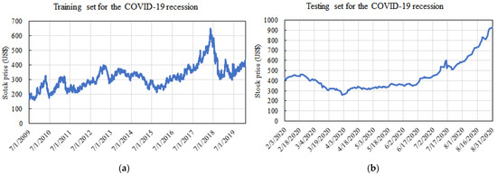
Figure 2.
Evolution of training set (a) and testing set (b) over time for the Random Length stock price for the COVID-19 recession modeling.
Table 2 shows the descriptive statistics for the training and testing datasets used to model the COVID-19 recession period. There was an averaged increase in approximately USD 125.47 during the COVID-19 pandemic driven by governmental shelter-in-place orders and stay at home measures. Both datasets started to show a departure from normality with somewhat higher skewness and kurtosis. This was even more pronounced in the testing data with standard deviation of 150.38 and skewness of 1.43.
Table 2.
Descriptive statistics for the COVID-19 pandemic training and testing periods.
2.2. Long Short-Term Memory Recurrent Neural Network
The LSTM recurrent neural network was introduced by Hochreiter and Schmidhuber [21] to primarily overcome the problem of vanishing gradients in commonly used recurrent neural networks in which the models resembled an ordinary node, except that it is replaced by a memory cell (Figure 3). Since the introductory work of 1997, LSTM networks have been modified and popularized by many researchers with variations that include an optional forget gate and a peephole connection [22,23]. In this paper, we focus on LSTM with a forget gate.
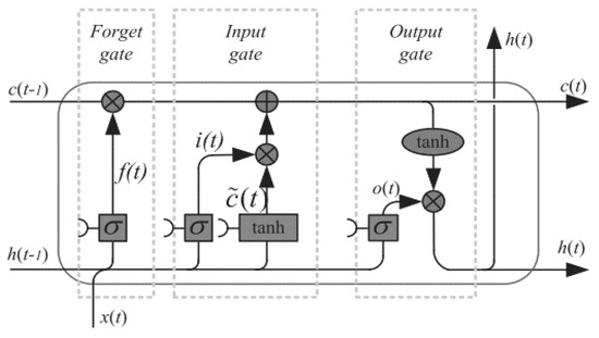
Figure 3.
A long short-term memory (LSTM) memory cell node with a forget gate (Yu et al., 2019).
The forget gate in Figure 3 provides a mechanism by which the network can learn to flush the contents of the internal state. The gate can decide what information will be thrown away from the cell state. The input gate is responsible for updating the cell state in which it decides what new information can be stored in the cell state, and the output gate decides what information can be output based on the cell state. On the basis of the connection in Figure 3, one can mathematically express the LSTM cell as follows:
- At time step t (t = 1, 2, …, T), given hidden state ht−1 past cell ct−1 from the last time step t − 1 and current input xt, the forward pass of LSTM is executed by first computing the updated memory cell čt:
- The input gate it controls how much information in č will flow through the new memory ct, and a forget gate ft is introduced to control what information in the previous cell ct−1 should be remembered:
- The output gate ot determines which part of the memory cell ct should flow into the hidden state ht:
2.3. Training and Evaluation
The entirety of the training and testing datasets were normalized to the range of 0 and 1 before training by
The network (Figure 4) was developed and trained using Python 3.6.5, TensorFlow 2.0 [24], and Keras 2.3.1 [25]. We tested 3 different timesteps—30, 60, and 120—which represents the total “memory” size of the closing price, in order to identify which resulting model would show best performance for predicting the great recession and the COVID-19 recession. Our model comprised a stack of 5 LSTM layers with 50 units in each layer, which corresponded to the dimensionality of the output space. The first layer was the input layer, which was the ordered 3-tuple (batch size, timesteps, feature), where batch size (i.e., the “?” symbol in Figure 4) represented the batch size that was set to a constant 256, and feature was set to a constant 1 that corresponded to the close price of the stock. The last layer was fully connected with only 1 node, which represented the time series stock price prediction.
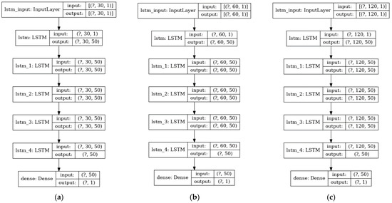
Figure 4.
Long Short-term Memory (LSTM) models with (a) 30 timesteps, (b) 60 timesteps, and (c) 120 timesteps.
We used the adaptive momentum estimator to iteratively minimize the mean squared error (MSE) loss function. The learning rate was set to 1 × 10⁻³ and reduced by a factor of 0.1 when the training loss stalled for 80 epochs. We stopped training when the training loss reached a plateau for 100 consecutive epochs. We trained the model on a single NVidia graphical processing unit (GPU).
Commonly used metrics to evaluate forecast accuracy are the mean squared error (MSE), root mean squared error (RMSE), and the mean absolute error (MAE). According to Bouktif et al. [26], RMSE is a metric that penalizes large error terms, and MAE is the mean of the sum of absolute differences between actual and forecasted values. The following metrics were then evaluated for each fold and recession period for the testing set.
where ŷi are the predicted values, yi, are the actual values, and N is the number of observations.
3. Results and Discussion
We first analyzed the feasibility of using long short-term memory artificial recurrent neural networks to predict Random Length lumber stock prices during the great recession period (2007–2009) and COVID-19 pandemic recession period (2020–). Figure 5 displays model performance during training.
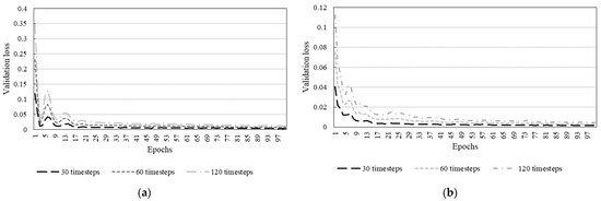
Figure 5.
Model performance for (a) great recession and (b) COVID-19 pandemic during training for each timesteps.
Figure 5 shows a high degree of learning from the network for both recession timeseries, confirmed by the observance of low mean squared errors (MSE). It is worth noting that the training of all timeseries for both recession periods behaved similarly after 100 epochs. We decided to include only 100 epochs for clarification as the validation losses become too small and hence overlap each other. For the great recession period, the MSE after training were 1.05 × 10⁻³, 6.35 × 10⁻⁴, and 6.94 × 10⁻⁴ for 30, 60, and 120 timesteps, respectively. For the COVID-19 recession period, the MSE after training were 1.15 × 10⁻⁴, 1.43 × 10⁻⁴, and 1.34 × 10⁻⁴ for 30, 60, and 120 timesteps, respectively. Furthermore, it is valid to infer that the models would perform relatively well on unseen data.
3.1. The Great Recession Period Analysis
The great recession period comprised data from 4 September 2007 up to 30 June 2009, which represented 430 datapoints to be predicted. Holidays and weekends were not predicted, as the stock market was not open for business during these periods. Figure 6 shows model predictions for different timesteps.
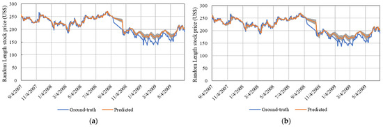
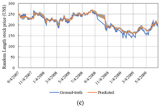
Figure 6.
Great recession prediction using LSTM for (a) 30 timesteps, (b) 60 timesteps, and (c) 120 timesteps. Shaded area represents standard deviation.
As observed in Figure 6, all timesteps performed very similar with the predicted value overlapping the ground-truth trend. Overall, the network with 120 timesteps performed better with lower error values (Table 3). Thereby, we can infer that longer timesteps have the capability of storing useful information that helps to capture the trend in future data for longer periods. However, in terms of computational processing, 30 timesteps is preferable, mainly due to the minimal error found between 30 and 120 timesteps.
Table 3.
Performance metrics for each timesteps during the great recession.
It is also clearly noted that the models did not perform well between September and early November 2008, regardless of timesteps. During the months of September and October 2008, the stock market reached its negative peak, which culminated with the stock market crash on 29 September 2008 affecting the following days [27]. Usually during normal operation, the stock market is open for business for approximately 21 days per month. In September and October 2008, the stock market was open for 10 days in each month.
3.2. COVID-19 Recession Analysis
The COVID-19 recession is an ongoing recession as of October 2020. We analyzed data from 3 February 2020 up to 3 September 2020, which corresponded to 147 datapoints to be predicted. Holidays and weekends were not predicted, as the stock market was not open for business during these periods.
Figure 7 shows that overall, the models had similar performance when predicting the Random Length stock price from February to middle September 2020. The models also captured the concomitant raise in the price of lumber that initiated approximately in middle June 2020 up to middle to late August. However, from this point and forward, the models diverged. The reason for such divergence is explained by the training set. The training set for the COVID-19 recession did not include such high variations. Machine-learning models are highly restricted with respect to predictions. In other words, the model only predicts what it learned from the training set. Table 4 shows the model’s metrics for each timesteps.
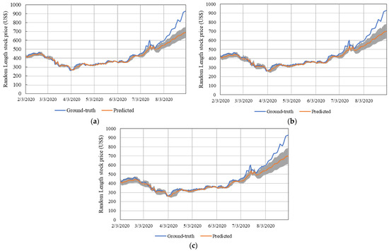
Figure 7.
COVID-19 recession period prediction using LSTM for (a) 30 timesteps, (b) 60 timesteps, and (c) 120 timesteps. Shaded area represents standard deviation.
Table 4.
Performance metrics for each timesteps during the COVID-19 recession.
Regarding the divergence observed, we primarily highlight the final prediction. The three models predicted the final price around USD 680, when it was around USD 918. Perhaps, this could be avoided by using even longer timesteps or deeper machine-learning models. Overall, the 30 timesteps model achieved better performance for the COVID-19 recession period with MSE, RMSE, and MAE of 0.0166, 0.1223, and 0.0711, respectively. When analyzing regression-like problems, these metrics should be close to 0. Furthermore, we consider the three models as appropriate to capture the trend in the data.
4. Conclusions
We demonstrated the feasibility of predicting the Random Length lumber stock price timeseries using LSTM artificial recurrent neural networks. Model training was based on daily data that incorporated the close price of the stock. We introduced three timesteps, namely, 30, 60, and 120 days to predict lumber price during two recent recession periods in U.S history, namely, the great recession in 2007–2009 and the current COVID-19 pandemic up to 31 August 2020.
It was observed that the three timesteps generated useful, efficient, and robust predictions of the stock price during the recession periods. LSTM networks are quite unique in the wood science field, and we showed this type of network is able to efficiently capture non-linear temporal relationships. The results achieved for both periods are remarkable with low error terms for MSE, RMSE, and MAE. Timeseries forecast is important for forest and forest products inventory management. It will help loggers, sawmills, and the transportation sector plan their activities without the need of understanding complex factors that underly the stock market. We plan to continue applying machine-learned algorithms in the wood science field such that every segment of the industry can be optimized with state-of-the-art techniques. For future applications, we plan to add factors that may influence the lumber price so that we would have a better understanding in their relationships.
5. Disclaimer
The authors would like to point out that financial instruments involve high risk, including the risk of losing some, or all, of someone’s investments, and thus may not be suitable for all investors. Stock prices such this one studied in this research are extremely volatile and may be affected by factors not covered in this research such as weather, financial and political events, and regulations. Before making any trading decision with the model provided herein, one should be fully informed of the risks and costs associated with trading in the stock market. Furthermore, the authors suggest that one takes careful consideration of investments goals, level of experience, and risk appetite. If one is interested in following the model, we urge them to seek professional advice where needed. The data herein are not provided by any market or exchange but may be provided by market makers, and thus prices may be not accurate and may differ from the actual given market price.
Author Contributions
Conceptualization, D.J.V.L.; methodology, D.J.V.L.; validation, D.J.V.L.; investigation, D.J.V.L.; writing—original draft preparation, D.J.V.L., G.d.S.B., and A.P.V.B.; writing—review and editing, D.J.V.L., G.d.S.B., and A.P.V.B. All authors have read and agreed to the published version of the manuscript.
Funding
This research was funded by the U.S. Department of Agriculture (USDA); Research, Education, and Economics (REE); Agriculture Research Service (ARS); Administrative and Financial Management (AFM); Financial Management and Accounting Division (FMAD); and Grants and Agreements Management Branch (GAMB), under agreement grant number 58-0204-6-001.
Institutional Review Board Statement
Not applicable.
Informed Consent Statement
Not applicable.
Data Availability Statement
The data and Python implementation can be seen at https://github.com/dvl23/lumber_prices_LSTM.
Acknowledgments
The authors wish to acknowledge the partial support of the U.S. Department of Agriculture (USDA); Research, Education, and Economics (REE); Agriculture Research Service (ARS); Administrative and Financial Management (AFM); Financial Management and Accounting Division (FMAD); and Grants and Agreements Management Branch (GAMB), under agreement no. 58-0204-6-001. Any opinions, findings, conclusions, or recommendations expressed in this publication are those of the author(s) and do not necessarily reflect the view of the U.S. Department of Agriculture. This publication is a contribution of the Forest and Wildlife Research Center (FWRC) at Mississippi State University.
Conflicts of Interest
The authors declare no conflict of interest.
References
- Alsharef, A.; Banerjee, S.; Uddin, S.M.J.; Albert, A.; Jaselskis, E. Early Impacts of the COVID-19 Pandemic on the United States Construction Industry. Int. J. Environ. Res. Public Health 2021, 18, 1559. [Google Scholar] [CrossRef] [PubMed]
- Fowke, C. National Association of Home Builders (NAHB) Warns That Record-High Lumber Prices Could Drive Up Housing Costs. Builder Online. 9 October 2020. Available online: https://www.builderonline.com/builder-100/leadership/nahb-warns-that-record-high-lumber-prices-could-drive-up-housing-costs (accessed on 25 March 2021).
- Hassan, M.R.; Nath, B. Stock market forecasting using hidden Markov model: A new approach. In Proceedings of the 5th International Conference on Intelligent Systems Design and Applications (ISDA’05), Warsaw, Poland, 8–10 September 2005; pp. 192–196. [Google Scholar]
- Trading Economics. Available online: https://tradingeconomics.com/commodity/lumber (accessed on 1 July 2020).
- Howard, J.L.; Westby, R.M.U.S. Timber Production, Trade, Consumption and Price Statistics 1965–2011; United States Department of Agriculture Forest Service: Washington, DC, USA, 2013; pp. 1–91.
- Ramage, M.H.; Burridge, H.; Busse-Wicher, M.; Feredaya, G.; Reynolds, T.; Shaha, D.U.; Wud, G.; Yuc, L.; Fleminga, P.; Densley-Tingley, D.; et al. The wood from the trees: The use of timber in construction. Renew. Sustain. Energy Rev. 2017, 68, 333–359. [Google Scholar] [CrossRef]
- Nagarajan, K.; Prabhakaran, J. Prediction of Stock Price Movements using Monte Carlo Simulation. Int. J. Innov. Technol. Explor. Eng. IJITEE 2019, 8, 2012–2016. [Google Scholar]
- Adebiyi, A.A.; Adewumi, A.O.; Ayo, C.K. Comparison of ARIMA and artificial neural networks models for stock price prediction. J. Appl. Math. 2014, 2014, 1–7. [Google Scholar] [CrossRef]
- Tadayon, M.; Pottie, G.J. Predicting student performance in an educational game using a hidden Markov model. IEEE Trans. Educ. 2020, 63, 299–304. [Google Scholar] [CrossRef]
- White, H. Economic prediction using neural networks: The case of IBM daily stock returns. ICNN 1988, 2, 451–458. [Google Scholar]
- Chiang, W.C.; Urban, T.L.; Baldrige, G.W. A neural network fund net asset approach to mutual value forecasting. Omega 1996, 24, 205–215. [Google Scholar] [CrossRef]
- Kim, S.H.; Chun, S.H. Graded forecasting using an array of bipolar predictions: Application of probabilistic neural networks to a stock market index. Int. J. Forecast. 1998, 14, 323–337. [Google Scholar] [CrossRef]
- Bandara, K.; Bergmeir, C.; Smyl, S. Forecasting across time series databases using recurrent neural networks on groups of similar series: A clustering approach. Expert Syst. Appl. 2018, 140, 112896. [Google Scholar] [CrossRef]
- Verizon Media—Yahoo! Finances. Available online: https://finance.yahoo.com/quote/LBS%3DF/history?p=LBS%3DF (accessed on 5 September 2020).
- Pedregosa, F.; Varoquaux, G.; Gramfort, A.; Michel, V.; Thirion, B.; Grisel, O.; Blondel, M.; Prettenhofer, P.; Weiss, R.; Dubourg, V.; et al. Scikit-learn machine learning in Python. J. Mach. Learn. Res. 2011, 12, 2825–2830. [Google Scholar]
- National Bureau of Economic Research. Available online: https://www.nber.org/news/business-cycle-dating-committee-announcement-june-8-2020 (accessed on 22 August 2020).
- Ng, S.; Wright, J.H. Fact and challenges from the great recession for forecasting and macroeconomic modeling. J. Econ. Lit. 2013, 51, 1120–1154. [Google Scholar] [CrossRef]
- Rich, R. The Great Recession. 2013. Available online: https://www.federalreservehistory.org/essays/great-recession-of-200709 (accessed on 15 July 2020).
- National Bureau of Economic Research. NBER Determination of the February 2020 Peak in Economic Activity. Available online: https://www.nber.org/sites/default/files/2020-11/june2020 (accessed on 30 July 2020).
- Gopinath, G. The Great Lockdown: Worst Economic Downturn Since the Great Depression; International Monetary Fund: Washington, DC, USA, 2020; Available online: https://blogs.imf.org/2020/04/14/the-great-lockdown-worst-economic-downturn-since-the-great-depression/ (accessed on 15 July 2020).
- Hochreiter, S.; Schmidhuber, J. LSTM can solve hard long-time lag problems. In Advances in Neural Information Processing Systems 9, Proceedings of the Annual Conference on Neural Information Processing Systems, Denver, CO, USA, 2–5 December 1996; NIPS: Islamabad, Pakistan, 1996; pp. 473–479. [Google Scholar]
- Gers, F.A.; Schmidhuber, J. Recurrent nets that time and count. In Proceedings of the IEEE-INNS-ENNS International Joint Conference on Neural Networks, IJCNN 2000, Neural Computing: New Challenges and Perspectives for the New Millennium, Como, Italy, 24–27 July 2000; Volume 3, pp. 189–194. [Google Scholar]
- Gers, F.A.; Schmidhuber, J.; Cummins, F. Learning to forget: Continual prediction with LSTM. In Proceedings of the 1999 Ninth International Conference on Artificial Neural Networks ICANN 99, Edinburgh, UK, 7–10 September 1999; pp. 850–855. [Google Scholar]
- Abadi, M.; Agarwal, A.; Barham, P.; Brevdo, E.; Chen, Z.; Citro, C.; Corrado, G.S.; Davis, A.; Dean, J.; Devin, M.; et al. Tensorflow: Large-scale machine learning on heterogeneous distributed systems. arXiv Prepr. 2016, arXiv:1603.04467. [Google Scholar]
- Chollet, F. Keras. GitHub. 2015. Available online: https://github.com/keras-team/keras (accessed on 9 July 2020).
- Bouktif, S.; Fiaz, A.; Ouni, A.; Serhani, M.A. Optimal deep learning LSTM model for electric load forecasting using feature selection and genetic algorithm: Comparison with machine learning approaches. Energies 2018, 11, 1636. [Google Scholar] [CrossRef]
- Lusk, V. The Market Crash of 2008 Explained. Wealthsimple. 2020. Available online: https://www.wealthsimple.com/en-us/learn/2008-market-crash (accessed on 27 July 2020).
Publisher’s Note: MDPI stays neutral with regard to jurisdictional claims in published maps and institutional affiliations. |
© 2021 by the authors. Licensee MDPI, Basel, Switzerland. This article is an open access article distributed under the terms and conditions of the Creative Commons Attribution (CC BY) license (https://creativecommons.org/licenses/by/4.0/).