Annual Shoot Segmentation and Physiological Age Classification from TLS Data in Trees with Acrotonic Growth

Abstract

The development of terrestrial laser scanning (TLS) has opened new avenues in the study of trees. Although TLS provides valuable information on structural elements, fine-scale analysis, e.g., at the annual shoots (AS) scale, is currently not possible. We present a new model to segment and classify AS from tree skeletons into a finite set of “physiological ages” (i.e., state of specialization and physiological age (PA)). When testing the model against perfect data, 90% of AS year and 99% of AS physiological ages were correctly extracted. AS length-estimated errors varied between 0.39 cm and 2.57 cm depending on the PA. When applying the model to tree reconstructions using real-life simulated TLS data, 50% of the AS and 77% of the total tree length are reconstructed. Using an architectural automaton to deal with non-reconstructed short axes, errors associated with AS number and length were reduced to 5% and 12%, respectively. Finally, the model was applied to real trees and was consistent with previous findings obtained from manual measurements in a similar context. This new method could be used for determining tree phenotype or for analyzing tree architecture.

1. Introduction

Trees are modular organisms that exhibit organ specialization in order to fulfill multiple functions [1]. Among these functions, the fulfillment of space exploitation (i.e., light interception) and space exploration requires the production of different types of vegetative axes, some being specialized for space exploration—long axes with a strong investment in woody structure and supporting many ramifications—and some for space exploitation—short axes with a strong investment in leaves, usually poorly or not branched [1,2,3,4,5]. These specialized axes are located on a morphogenetic gradient that can be partitioned into a finite number of “physiological ages” that express the stage of differentiation of the meristem that produced an axis. Therefore, a physiological age (PA) is characterized by a particular combination of morphological and anatomical attributes related to the function of this specific PA [1]. Studying the role, interactions, and complementarity between PAs requires cross-scale analyses (e.g., [5]). However, obtaining such data for an entire tree remains challenging as these measurements are typically very time consuming. However, the recent development of terrestrial laser scanning (TLS) holds great potential for overcoming this limitation as 3D data of tree structures at a very high spatial resolution can be quickly acquired.

In recent years, TLS has received increasing attention from foresters, forest ecologists, and urban foresters for extracting geometrical properties and deriving morphological or functional metrics at the stand or tree level. At the tree level, TLS has been used to estimate tree dimensions [6,7], tree volume and biomass [8,9,10,11,12,13], tree shape and space occupancy [14,15,16,17], tree leaf area [18,19,20,21,22], or the within tree light transmittance [23,24]. In most of these studies, TLS was used to analyze the tree shape and architecture at the tree scale [25] or to analyze the architecture of the trunk and main branches [26]. However, the physiological age of a botanic entity is described at the growth unit or annual shoot level [1]. To obtain information on the PA at the whole tree level, growth unit or annual shoot need to be segmented from TLS data.

Among the TLS data treatment methods currently available, some enable tree skeleton extraction, i.e., an ensemble of segments of the tree structure [27,28,29,30], or to build a quantitative structural model (QSM), i.e., an assemblage of cylinders [31,32,33,34]. While skeletonization methods are often used as a basis for QSM method implementation, the latter are widely used to quantify the general branch architecture [10,26] or the tree volume and biomass [8,11,35,36,37,38]. These models can also serve as support to radiative transfer modeling when foliage is added to a QSM or a skeleton [22,39,40,41,42]. However, these methods have never been used to assess topological and architectural information at a scale as small as the annual shoot.

As QSMs and skeletons are a set of cylinders or segments, a basic topology (i.e., the hierarchy among cylinders or segments), that can generally be stored by the models or be easily retrieved from the final model. This simple topological information could serve as the basis to implement an annual shoot segmentation model from which more complex topological and morphological information could be derived. To do so, we developed a new workflow that aims to detect the branching patterns created by the acrotony, i.e., the preferential development of the lateral axes located at the distal part of a growth unit [1], in order to segment annual shoots from a tree skeleton. Such an approach thus aims (i) to analyze the simple geometric and topological information available in QSMs and skeletons to segment annual shoots, (ii) to use manual measurements of annual shoot length to retrieve the PA of the segmented annual shoot, and (iii) to add the non-reconstructed axes to the QSM or skeleton using a simple architectural automaton. The model is designed to be used on TLS scans acquired during the leaf-off period as it helps to offset foliage-induced occlusion and to obtain more accurate woody structure reconstructions [40].

We also provide a validation of the method at various levels of the tree architecture, ranging from the annual shoot level to the entire tree level. Since a quantitative assessment of the tree architecture (i.e., number of axes, internodes, or their position) is very hard to obtain for large trees, we used simulated tree structures to simulate TLS scans in a context comparable to field conditions. This method is based on the simulation of TLS scans on realistic simulated tree structures produced with a tree architecture simulation model. We then provide an example of its application in a tree trimming experiment.

2. Description of the Annual Shoot Segmentation Model

The annual shoots (AS) segmentation model considers only segments. Consequently, the term “tree skeleton” is used similarly for QSM and strict skeletonization. A tree skeleton is a set of segments within which two types of objects can be described (Figure 1):

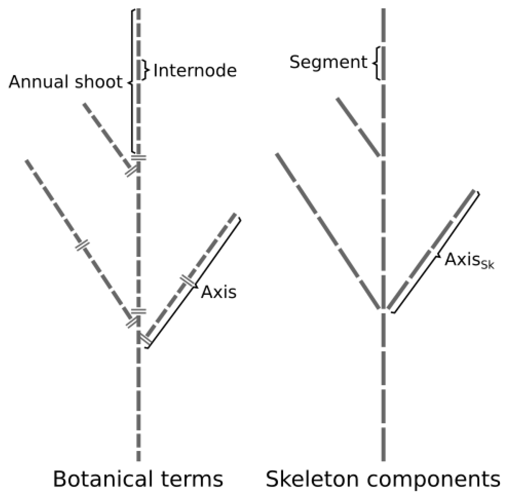
• The segment that is the elementary element of a skeleton defined by 3D coordinates of its starting and ending points and by its unique identifier.
• The skeleton’s axes (axes${}_{Sk}$) are a linear assemblage of connected segments starting from a branching point (or at the tree base for the trunk) and ending at a tip of the skeleton (i.e., a segment without a child segment).

The annual shoot segmentation and classification method is based on 7 steps that can be separated into three main main sections:

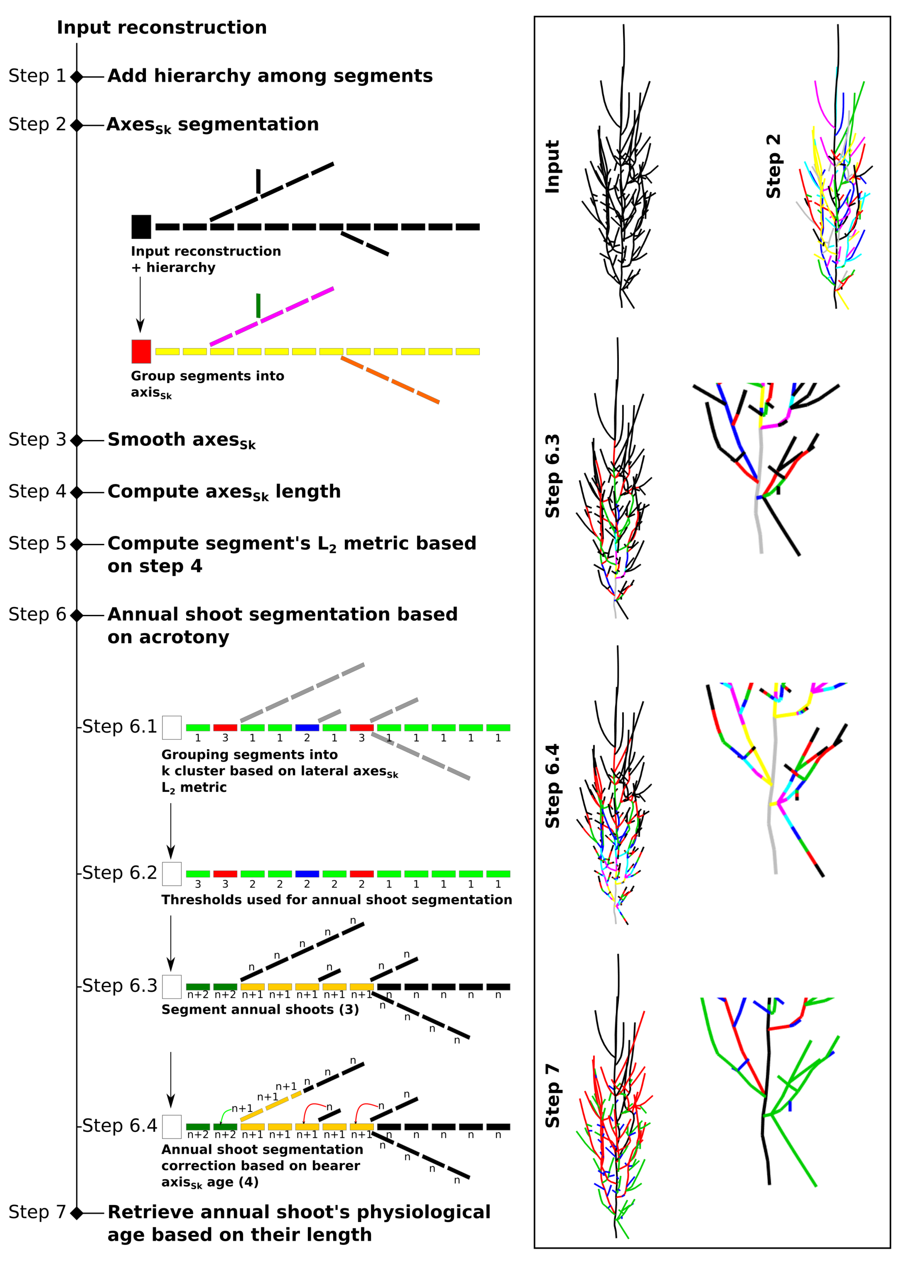
• data preparation prior to annual shoot segmentation (steps 1 to 4)
• annual shoot segmentation (steps 5 and 6)
• annual shoot classification into physiological ages (step 7)

The flowchart of these steps is illustrated in Figure 2.

2.1. Data Preparation Prior to Annual Shoot Segmentation (Steps 1 to 4)

Step 1. By default, a skeleton is composed of only segments, and, the axes${}_{Sk}$ have to be retrieved from a hierarchy among the segments and the geometry of the skeleton. To do so, the hierarchy among connected segments (i.e., parent/child relationships) is first computed for the entire skeleton (Figure 2, Step 1).

Step 2. Segments are then grouped into axes${}_{Sk}$ using an iterative hierarchical process so that an axis always follow the longest path from its starting point to a branch tip (Figure 2, Step 2). Starting with the segment (S${}_{init}$) wtih the smallest z value (i.e., the trunk basis), the child segment that bears the longest branched system (longest in terms of the cumulative length) among all child segments (S${}_{children}$) is assumed to belong to the parent segment’s axis${}_{Sk}$. This process continues until no S${}_{children}$ are found (i.e., the axis tip is reached), and the process restarts with a new S${}_{init}$ being an unclassified child of an already classified segment.

Step 3. Once axes${}_{Sk}$ are segmented, the skeleton is smoothed in order to improve further axis length computation. To do so, the segment tip and base of the axes${}_{Sk}$ are displaced in order to reduce the deviation between three successive axis segments (see Figure 3 for an illustration). This step is performed iteratively until no additional modifications are conducted.

Step 4. After skeleton smoothing, the geodesic distance of each axis${}_{Sk}$ segment tip relative to the axis${}_{Sk}$ base is computed, as is the number of child axes${}_{Sk}$ of each segment of the structure (Figure 2, Step 4).

Figure 2. Illustration of the entire workflow (seven steps) involved in the annual shoot segmentation and physiological age classification model. On the left, a complete list of steps and illustrations of some steps and substeps of the algorithm. On the right, screen shots of the skeleton of a real tree at the end of key steps showing the entire tree and, in some cases, the detail of the tree base. In the screen shots, the colours correspond to the axis ID (step 2), the segmented annual shoots before non-branches axes correction (step 6.3), the corrected annual shoot segmentation (step 6.4), and the physiological ages (step 7, PA1 in black, PA2 in red, PA3 in green, and PA4 in blue). Note that substeps 6.1, 6.2, and 6.3 are illustrated in more detail in Figure 4.

Figure 2. Illustration of the entire workflow (seven steps) involved in the annual shoot segmentation and physiological age classification model. On the left, a complete list of steps and illustrations of some steps and substeps of the algorithm. On the right, screen shots of the skeleton of a real tree at the end of key steps showing the entire tree and, in some cases, the detail of the tree base. In the screen shots, the colours correspond to the axis ID (step 2), the segmented annual shoots before non-branches axes correction (step 6.3), the corrected annual shoot segmentation (step 6.4), and the physiological ages (step 7, PA1 in black, PA2 in red, PA3 in green, and PA4 in blue). Note that substeps 6.1, 6.2, and 6.3 are illustrated in more detail in Figure 4.

Figure 3. Illustration of the structure smoothing for three axis segments. If a modification is needed (i.e., the case illustrated at the bottom), the point that makes the junction between the second and third axis segments is moved to the averaged location between the base of the second and the tip of the third axis segment.

Figure 3. Illustration of the structure smoothing for three axis segments. If a modification is needed (i.e., the case illustrated at the bottom), the point that makes the junction between the second and third axis segments is moved to the averaged location between the base of the second and the tip of the third axis segment.

Figure 4. Illustration of the annual shoot segmentation along the trunk of an 8-year-old simulated tree composed of 105 segments. The input data (a) consists of a set of segments (dots of a dashed line), here presented with a schematic representation of their child axes${}_{Sk}$ (with the axes${}_{Sk}$ in green being used in the L${}_2$ metric computation and those in red being excluded). Note that the annual shoots of the main axis are represented by a bicolour line for the purpose of clarity. The L${}_2$ metric of each segment is then computed (bar height in (b)). The segments are then grouped into clusters based on their L${}_2$ metric, and the clusters are ranked by increasing order of L${}_2$ metric (bar height in (c)). An evolutive threshold (black line in (c)) is then used to identify the tips of the annual shoots (arrows in (c). The output is the segmented annual shoots (shown in black and grey in (d)). Note that the annual shoots located near the tree base are not segmented by the method as the trunk base is not branched (compare annual shoots in (d) to those in (a)). Note that the steps indicated on the left of the figure correspond to the steps illustrated in Figure 2.

Figure 4. Illustration of the annual shoot segmentation along the trunk of an 8-year-old simulated tree composed of 105 segments. The input data (a) consists of a set of segments (dots of a dashed line), here presented with a schematic representation of their child axes${}_{Sk}$ (with the axes${}_{Sk}$ in green being used in the L${}_2$ metric computation and those in red being excluded). Note that the annual shoots of the main axis are represented by a bicolour line for the purpose of clarity. The L${}_2$ metric of each segment is then computed (bar height in (b)). The segments are then grouped into clusters based on their L${}_2$ metric, and the clusters are ranked by increasing order of L${}_2$ metric (bar height in (c)). An evolutive threshold (black line in (c)) is then used to identify the tips of the annual shoots (arrows in (c). The output is the segmented annual shoots (shown in black and grey in (d)). Note that the annual shoots located near the tree base are not segmented by the method as the trunk base is not branched (compare annual shoots in (d) to those in (a)). Note that the steps indicated on the left of the figure correspond to the steps illustrated in Figure 2.

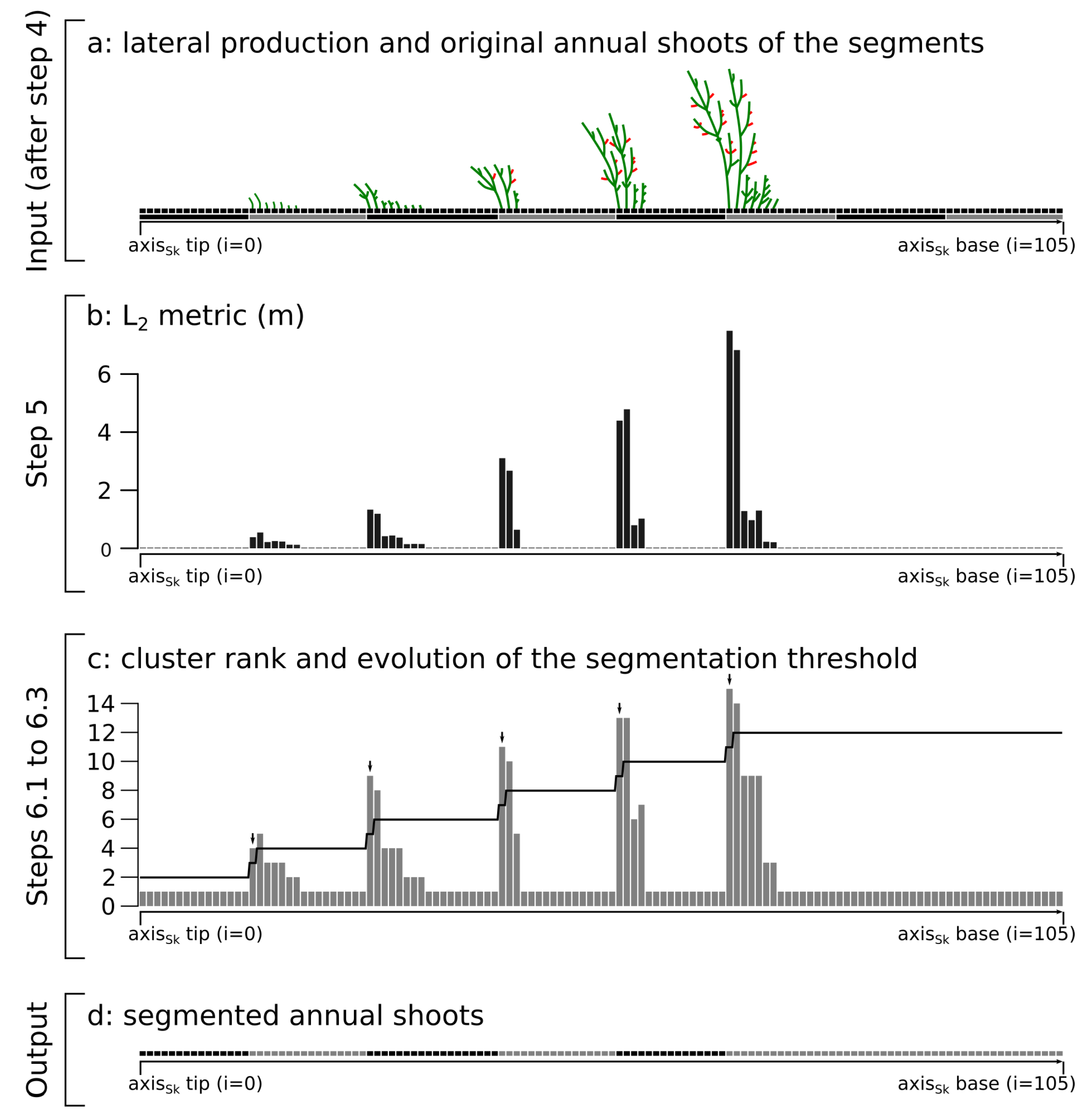
2.2. Annual Shoot Segmentation (Steps 5 and 6)

As in many temperate species an AS corresponds to a single growth unit, the AS segmentation is based on acrotony and therefore relies on the following assumptions:

• acrotony occurs at least on the main axes of the tree structure

  -

  the longest lateral axes are close to the AS tip,

  -

  an AS ends immediately or shortly after the last branching point, and 

  -

  annual shoots are composed of only one growth unit (i.e., there is no polycyclism) so that branching occurs close to the tip of the AS.

• an AS produced at year n can only bear an AS produced at year $n+1$

Based on these assumptions, we developed a model that detects the branching patterns of a given axis and deduces the position of an AS tip from these patterns using very simple rules and without the need for external parameters.

Step 5. For each segment of an axis${}_{Sk}$, a metric describing the length of its child axes${}_{Sk}$ is first computed. This metric corresponds to the length of the lateral axes${}_{Sk}$ of the segment plus the length of their respective child axes${}_{Sk}$. As this metric refers to the length of the child axes of order $BO+1$ and $BO+2$ ($BO$ being the branching order of the target segment), we refer to it as the secondary order length (L${}_2$ metric, Figure 4a,b). The L${}_2$ metric is used as it captures the lateral axes complexity better than the length of the main axis${}_{Sk}$ while reducing the importance of the skeleton quality variations when comparing two lateral axes${}_{Sk}$, e.g., when comparing the length of an axis${}_{Sk}$ located in a poorly reconstructed part of the skeleton (due to low point cloud density) to the length of a better-defined axis${}_{Sk}$.

Step 6.1. After computation of the L${}_2$ metric, segments are grouped into k clusters based on their L${}_2$ metric. This transformation allows us to group segments with similar L${}_2$ metric, which enables us to mitigate the effect of small differences in L${}_2$ when comparing two segments. This also allows us to apply a simple thresholding approach to segment annual shoots, which results in simpler and more robust AS segmentation than if it is based on the raw L${}_2$ metric. The clustering is performed using hierarchical aggregative clustering with Ward’s method [43,44] (Figure 4c), implemented in R in the hclust function [45]. This method iteratively groups single observations by minimizing the within-group dispersion at each fusion. The resulting dendrogram is then pruned in order to maintain k clusters. In the model, the optimal k is defined as the minimal number of clusters so that every non-branched segment (i.e., with L${}_2$ = 0) is grouped into one single cluster. This approach was found to be more efficient than partitioning clustering methods (e.g., regression trees) for quickly isolating non-branched segments to produce a reasonably small k and was favoured over non-hierarchical clustering methods (e.g., k-means) as the latter usually performs better in multidimensional space. Clusters are then ranked based on their L${}_2$ so that $C1$ has an average L${}_2$ of 0 and $C2<C3<C4<\dots <Ck$ (Figure 4 compares cluster rank in c to L${}_2$ in b).

Steps 6.2 and 6.3. The clusters are then used as the basis for AS segmentation. In acrotony, lateral axes located at the tip of an AS are expected to be longer than those located near the base of the AS. At the same time, lateral axes that initiate near the base of the parent axis are older, so they are expected to have a larger L${}_2$ metric and, therefore, belong to a higher cluster. To accommodate these two nested patterns, an evolutive threshold (t) is used. It starts with a value $t_0=2$, and, moving from the axis tip to the axis base, a new AS tip is added to the segment $S_i$ if $C_i\ge t_i$ and $C_{i-1}<t_i$, and at the same time $t_i=t_{i-1}+1$, $if{C}_i>t_i$ (see Figure 4c for an illustration).

During the AS segmentation steps, three cases can occur:

• The AS are correctly segmented. This is usually the case for axes${}_{Sk}$ of small order (i.e., main branches and trunk). This is because large axes usually bear many child axes, which are usually well reconstructed by skeletonization methods and because branching accidents are relatively rare in axes of lower order.
• The AS are not segmented. This is typically the case for axes${}_{Sk}$ of higher order (i.e., short axes) that are usually not branched or poorly branched. This results in an AS longer than it should be (compare steps 6.4 to 6.3 in Figure 2).
• Oversegmentation (i.e., the addition of an AS that does not exists in reality) occurs. This results in an AS shorter than it should be, usually one segment long and mostly occurring at the tip of an annual shoot.

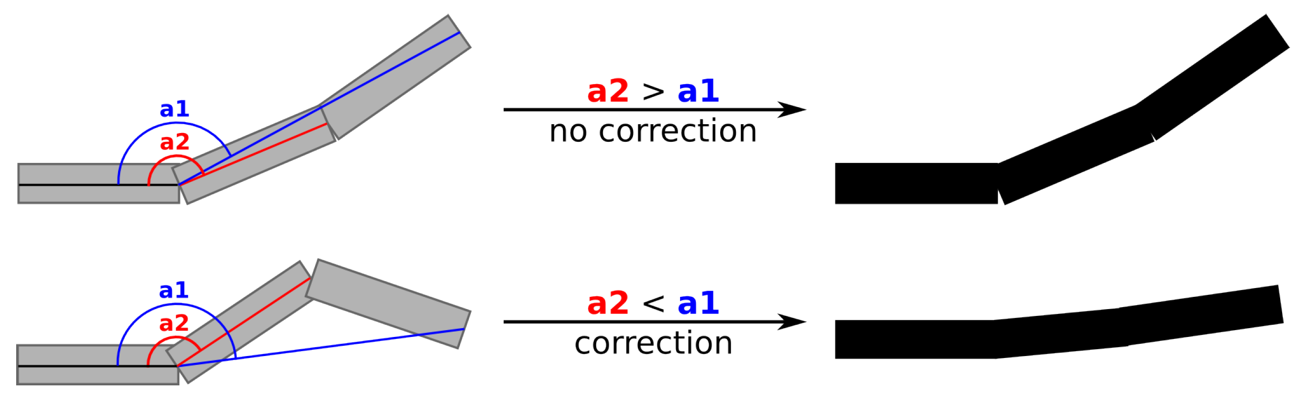
Step 6.4. After AS segmentation, each axis${}_{Sk}$ is tested for potential segmentation errors. This test is based on assumptions that the segmentation of the main axis${}_{Sk}$ (that starts at the tree base and ends at the tip of the skeleton) is perfect and that an AS produced at year n can only bear AS produced at year $n+1$. For each axis, the year of the first AS is compared to the bearer of the annual shoot, and three results can occur depending on the above cases:

• if $beare{r}_{year}-chil{d}_{year}-1=0$, the annual shoots of the axis are correctly segmented (case 1)
• if $beare{r}_{year}-chil{d}_{year}-1>0$, some annual shoots are not segmented (case 2)
• if $beare{r}_{year}-chil{d}_{year}-1<0$, some supernumerary segmentation occurred (case 3)

When case 1 occurs, no correction is conducted. When case 2 occurs, an iterative correction is performed: while $beare{r}_{year}-chil{d}_{year}-1>0$, the longest AS is divided into equally sized AS. Note that, at each iteration, the results of the previous iteration are included so that two different AS can be segmented and not only the longest one. When case 3 occurs, the shortest AS is merged with the previous one except if the shortest AS is the first of the axis. In that latter case, the shortest AS is merged with the next AS.

As the corrections are made in increasing order of branching order (BO), i.e., from BO1 to the ultimate BO (according to the definition from [1]), the corrections propagate within the entire structure as the corrections made within a given BO are used to evaluate the segmentation accuracy in the next BO.

2.3. Classification of Physiological Ages

Step 7. A physiological age is then assigned to each segmented AS based on its length. A previous attempt to automatically retrieve AS types (a concept derived from the concept of PA) from field measurements was based on a combination of topological information and morphological measurements [5]. Other research has shown that morphological and functional variables scale with the AS length [2,3]. Therefore, in the present study, we decided to use the AS length as input for PA classification as it can be applied directly to the AS segmented in a skeleton. PA assignment thus requires the user to provide length thresholds that will be used to make the distinction between two PA. More details on the method we used to retrieve these thresholds from field measurement is provided in Section 3.1.2.

A topology-based correction of the PA of AS can optionally be performed after length-based PA classification. This can be required when wrong positioning of branching points in the skeleton causes the first annual shoot of an axis${}_{Sk}$ to be shorter than the corresponding AS in the real axis, resulting in a wrong classification of PA. The correction assumes that a given AS can only bear AS of equal or lower PA. The correction is performed iteratively by decreasing branching order as follows: if $P{A}_{child}<P{A}_{parent}\to P{A}_{parent}=P{A}_{child}$.

3. Material and Methods

We used two levels of validation for the model:

• at the tree and AS level using “perfect data”
• at the tree level using simulated TLS data

First, a tree simulation model was calibrated based on manual measurements of red ash trees (Fraxinus pennsylvanica). The simulated tree structures were then used in the annual shoot segmentation model. In this first validation step, the model was tested in perfect conditions as the input data is complete and geometrically perfect (i.e., free of skeletonization errors). For the second validation step, TLS scan simulations were conducted on the simulated trees. These simulated TLS scans were then used as input in two different QSM algorithms. The data obtained with the perfect data and QSMs were then compared to the original simulated tree structure.

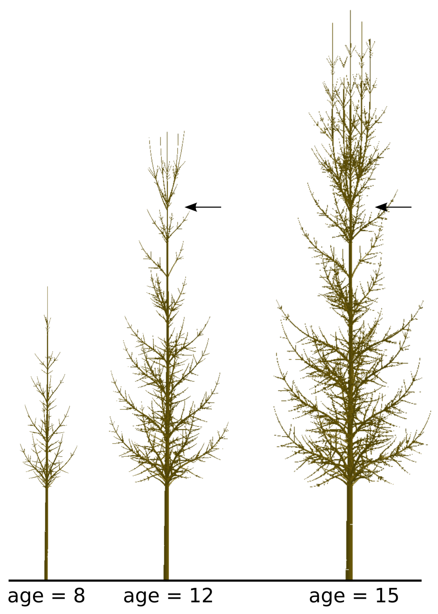
3.1. Tree Sampling, Modeling, and Physiological Age Classification

3.1.1. Sampled Trees and Architectural Measurements

Nine red ash trees (Fraxinus pennsylvanica “patmore”) growing at the nursery of the city of Montreal located in the city of l’Assomption, Quebec, Canada, were selected. Red ash was selected as a model species as its architecture and development are well documented [46] and because its strong acrotonic organization makes it a perfect model species to test our method. The trees were part of a trimming experiment aimed at replicating the tree trimming for power line maintenance. The trees were trimmed according to three intensities: 0% (i.e., control trees), 40%, and 70% of branch removal in 2015 (see [47] for more information). Thus, architectural measurements were taken on three trees for each of these treatments.

Nondestructive manual architectural measurements of three-year-old branched systems were taken in August 2017. To do so, axes of secondary branching order (i.e., BO2 [1]) were randomly selected. Note that BO2 axes includes sequential branches, sequential reiterations of the trunk, and delayed traumatic reiterations that emerge after trimming. This sampling plan ensures that data are obtained for A1 axes, which were generally inaccessible for measurements in control trees.

For each AS of the main axis of each BO2, measures were taken at the internode (IN) level: IN length; number of leaves; the length of one (usually over two) leaf; as well as the number, length, and basal diameter of its lateral axis. For each AS of the BO2 axis, one to six lateral axes were semi-randomly selected (with the criteria of varying axes size in order to increase the probability of sampling various physiological ages) for further measurements. For each selected lateral axis, similar measurements as that for the BO2 axis were performed. This resulted in a total of 117 axes measured at the internode level and a total of 175 axes measured at the axis level (i.e., with only total length, basal diameter, and number of leaves).

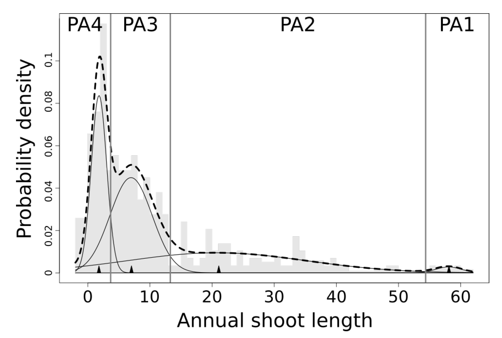
3.1.2. Physiological Age Classification from Manual Measurements

As previously explained, ASs were classified into PA based on their length only. To do so, we hypothesized that the frequency of occurrence of PAs varies within the branched systems, resulting in a PA classification based on the frequency distribution of AS length. Distribution mixture models (DMM) were used to fit four normal distributions to the AS length frequency distribution. Four distributions were used as this is the number of different axes types observed in red ash architecture [46]. Note, however, that we also tested the fit of the models with five distributions (i.e., four PAs in the sequential tree development and one delayed traumatic reiteration) but without success. The DMM was fitted to the complete measurements of the branched systems (i.e., 289 ASs retrieved from the manual measurements previously described) using the mixdist R package [48]. Note that none of the DMM parameters were fixed and could, consequently, take any value. The starting parameters for the DMM model fitting were as follows:

• mean value of the distribution: mu = 2 cm, 10 cm, 30 cm, and 50 cm
• standard deviation: sigma = 10
• the (optional) proportion of the data contained in each distribution (pi) is not provided

As we expect that different PAs will exhibit different morphological and functional attributes, the PA classification based on DMMs was assessed by comparing morphological and functional parameters of the current year AS: the AS leaf area (LA, cm${}^2$), the AS leaf area display (LAD, leaf area:length, cm${}^2$.cm${}^{-1}$), and the leaf-to-shoot ratio (L:S, leaf area:shoot volume, cm${}^2$.cm${}^{-3}$). As we used nondestructive measurements, this last indicator is assumed to be closely related to the leaf-to-shoot ratio (g.g${}^{-1}$) used in other studies [2,3], assuming a constant leaf mass per area and wood density. Note that the leaf area is obtained from the allometric relation of leaf length (r${}^2$ = 0.811). Kendall’s Tau ($\tau$) was used to estimate the correlation strength between the AS length and LA, LAD, and L:S as these relations are generally not linear. Pairwise comparisons of LA, LAD, and L:S as a function of the AS’s PA were then completed using the Kruskal–Wallis test as the residuals were not normally distributed. The analyses were completed using the kendall and kruskal functions from the agricolae R package [49].

3.1.3. Architectural Model Calibration

In order to evaluate the accuracy of the presented method, synthetic TLS data were produced in silico to obtain quantitatively (dimensions and amount of organs) and qualitatively (annual shoot types) known references. To do so, tree structures were simulated using the AmapSim model that produces botanically realistic tree models based on simple developmental rules [50]. The model calibration, which is based on previously described manual measurements of the branched systems of red ash trees, is detailed in the Supplementary Materials S1. Trees at 5 to 15 years of age were simulated. For each age, ten trees were simulated, resulting in a total of 110 simulated trees. A unique random seed was used for each individual simulation in order to avoid redundancy among trees of different ages. See Figure 5 for an example of simulated trees at different ages.

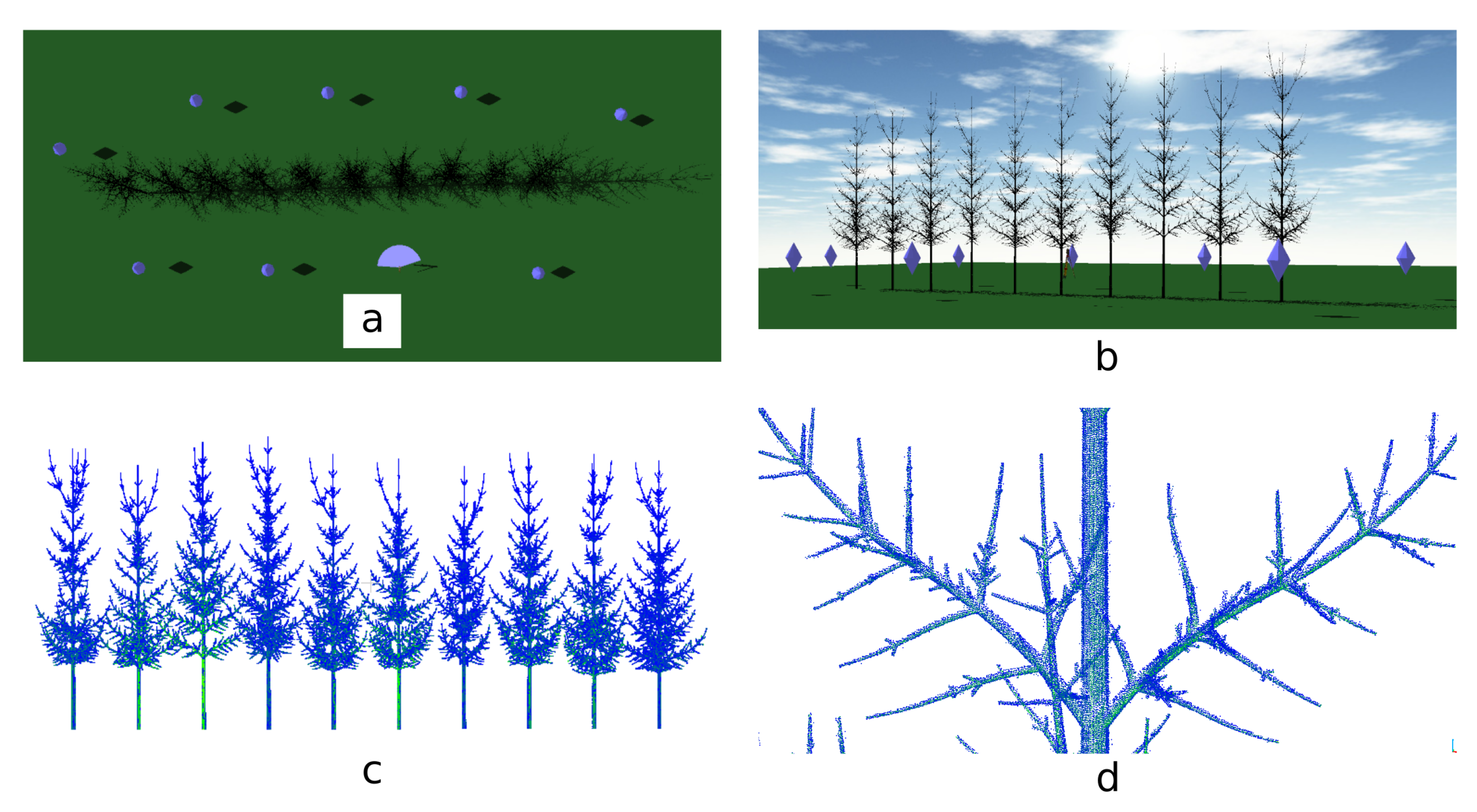
3.2. TLS Simulations

TLS simulations were performed using the Helios model [51] that simulates aerial, fixed or mobile terrestrial laser scanner to survey an artificial 3D scene. In order to build the 3D scene, a mesh object was created for each simulated tree from the output of the AmapSim model in R using the tools available in the rgl package [52]. Using trees ranging in age from 5 to 15 years, eleven 3D scenes were built, each containing ten trees of the same age. In each scene, the trees were organized into a single row with 4 m between the trees (Figure 6a,b). This distribution increases the overlap between the trees as they grow, mimicking trees typically grown in a row, as in a nursery or an orchard. The scanning conditions thus change when the trees becomes larger, as large trees are more prone to producing occlusions caused by crowns overlapping.

The TLS survey was then performed using nine scan positions. The positions were manually distributed in staggered rows around the tree row, the spacing between two scan positions being ~1.5 times the spacing between two trees, i.e., ~6 m, and the distance between a tree and the scanner position was 6 m (Figure 6a). The simulated TLS device was a FARO focus X130 with an angular resolution of 0.04${}^{°}$ in both the vertical and horizontal directions.

In the output of the Helios model, individual scans are registered within the same coordinate system and, consequently, no scan registration is required (Figure 6c). The simulated TLS scenes are then imported into the CloudCompare software [53]. Individual trees are manually segmented, and the statistical outliers filter (SOR) is used to remove noise from the simulated scans. The SOR filter is used to compute the distance of each point to its six nearest neighbours and the points with the average distance greater than 4 times the standard deviation are removed (see Figure 6d for clean point cloud details).

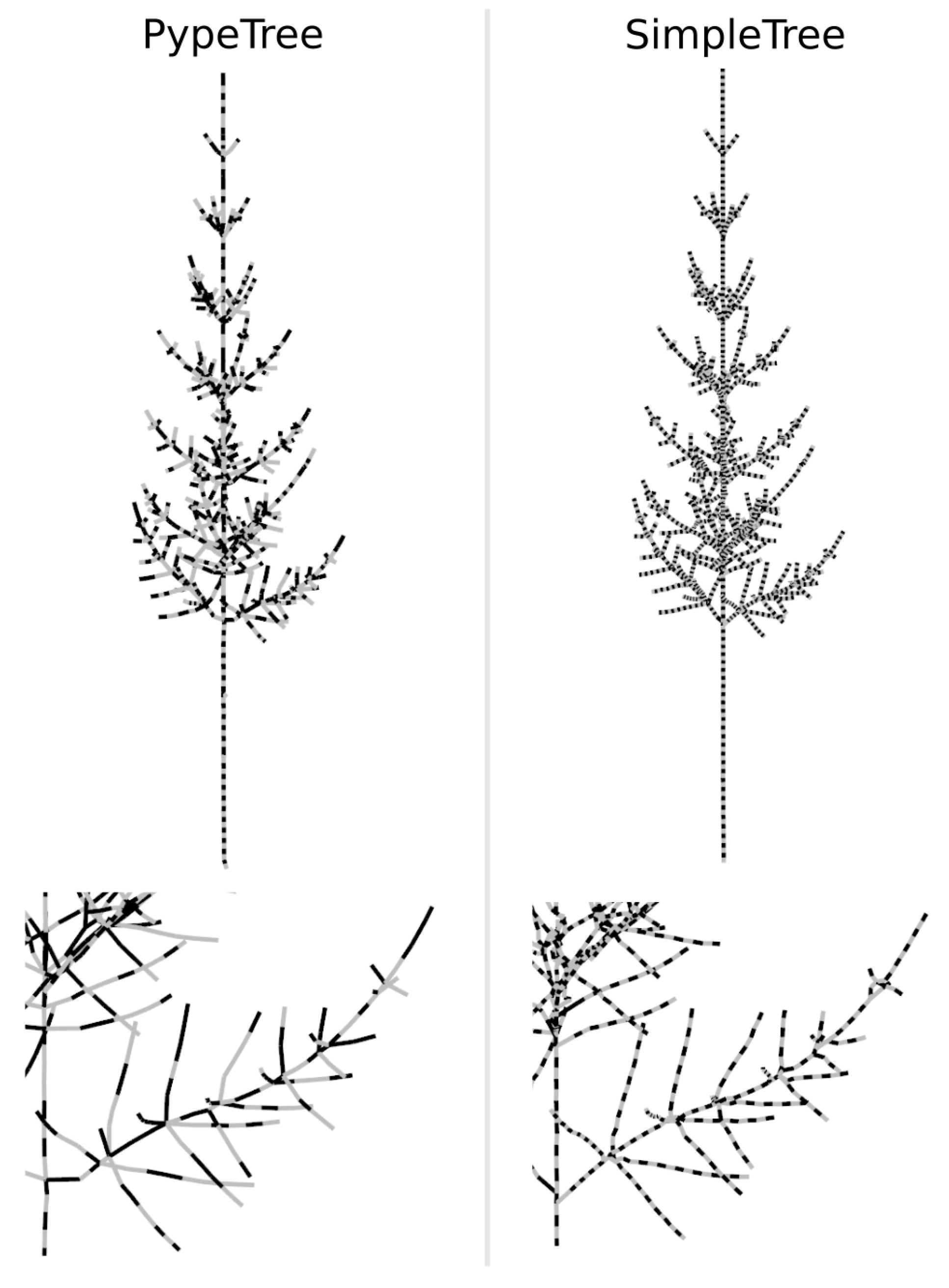
3.3. Simulated TLS Data Skeletonization

As the segment is a fundamental unit of a skeleton and of the AS segmentation model, it is possible that the skeletonization algorithm used to produce the skeleton would influence the results. Therefore, we used two different state-of-the-art and freely available QSM algorithms to produce tree skeletons from the simulated TLS data (The results of the two models can be compared in Figure 7).

PypeTree [32] is a semiautomatic QSM algorithm based on the construction of a geodesic graph [27]. Initially, the geodesic graph was constructed by connecting each point to its k nearest neighbours. k was set to 5 in our reconstructions, and we also applied a maximum search distance of 0.05 m (i.e., a point cannot be connected to a point located further than 5 cm even if it has less than 5 neighbours), which avoids connecting points located on two different branches. After computing the geodesic graph, it can be manually corrected by connecting non-connected components. In our reconstructions, we reduced the manual work to a minimum and only reconnected the largest components (i.e., non-connected branching order 2 or 3). In all trees, the manual work took less than 5 min. After building the geodesic graph, PypeTree computes the geodesic distance of each point to the trunk base. A second parameter, d, was then applied to discretize the geodesic distance. This creates “stages” within which non-connected components (clusters) are assumed to belong to a different branch. Each cluster is then used to produce a cylinder. In our reconstructions, d is set to 0.1 m, which appears to be a good compromise between the trunk diameter (a too-small d causes the creation of inconsistent branches on the trunk) and the axes length (as short axes annual shoots are 0.04 m long, they will be detected with high probability). Consequently, the length of the axes segments within skeletons obtained using the PypeTree algorithm are 0.1 m long. After all cylinders are built, PypeTree can be used to manually add missing cylinders and to “smooth” the structure. In our reconstructions, these two steps were not used as manually adding missing cylinders was considered too time consuming and structure smoothing is accomplished within our annual shoot segmentation model.

We used SimpleTree [33,54], implemented in CompuTree (version 5.0.140 [55]) as a second skeletonization algorithm. This method uses a “sphere following” algorithm (see [8,33] for extensive description of the method) to fit cylinders to the point cloud. In the version of SimpleTree available in the CompuTree platform, all the parameters are computed internally by the model so the user does not need to provide any parameters.

3.4. Comparisons of Modeled vs. Simulated Annual Shoots and Physiological Ages

The objective of the validation based on perfect data is to provide two levels of validation (i.e., at the AS level and at the tree level). The validation at the tree level is based on the cumulated length and total number of ASs for each PA. Validation at the AS level requires matching each segmented AS to the original AS in order (i) to compute the error rate in segmented AS estimated production year, (ii) to compute the PA classification error rate, (iii) to compute the AS length estimates error, and (iv) to determine how this error propagates among AS production years. This matching is based on the fact that the skeleton segments correspond to the internodes of the original data. Therefore, the matching between the segmented AS and the original AS is based on the number of shared segments/internodes: the AS of the original data corresponding to a given segmented AS is the one that shares the most segment/internodes. To do so, the AS segmentation algorithm arranges skeleton segments into annual shoots so that each AS is composed of a whole number of segments.

In validation based on the skeletons extracted using the PypeTree and the SimpleTree algorithms, matching an individual AS to the corresponding AS in the original data is not feasible as the skeleton’s segments substantially differ from the internode positions. Therefore, only variables at the tree scale are extracted (i.e., cumulated length and total number of AS in each PA) in order to compare both algorithms in terms of reconstruction quality (i.e., their ability to reconstruct different PAs). In this case, as the segment lengths can be longer than the internode lengths in the original data and because segment lengths vary among the two QSM algorithms (Figure 7), the segmented AS tips are interpolations of segment tip coordinates. In other words, if the tip of a segmented AS falls between the two extremities of a segment, this segment is partitioned into two smaller segments so that the length of the segmented AS is exactly the same as the one computed by the model.

In any case, the Mean Absolute Error (mae, $\sum \left|predictobserved\right|/n$), Mean relative Prediction Error (mpe, $(\sum (observed-predict)/observed)/n$) and/or Mean Absolute Percentage Error (mape, $(\sum |(observed-predict)/observed\left|\right)/n$) are used to evaluate the total PA length and number, and the individual annual shoot length estimate error.

3.5. Improving the Reconstruction through Non-Reconstructed Axes Modeling

In order to test the possibility of adding non-reconstructed PA4 axes to the tree skeleton, we implemented a simple architectural automaton. For each 2- to 5-year-old annual shoot of PA1, PA2, and PA3 of the reconstructed skeleton, a potential number of PA4 ($pPA4$) is compared to the reconstructed number of PA4 ($nPA4$), and if $pPA4>nPA4$, then $pPA4-nPA4$ randomly generated PA4 annual shoots are added to the tree skeleton. The model uses similar procedures to those of the AMAPsim model, and the parameters are the same as those used to simulate the trees (see Supplementary Materials S1):

• Markov chains were used to determine branching probabilities in order to estimate pPA4 and position modeled PA4 axes along an AS (using parameters shown in Supplementary Materials Figure S1b)
• binomial distributions were used to generate random PA4 ASs (using parameters shown in Supplementary Materials Figure S1c)

Twenty random simulations were performed for each tree, and the average number and length of AS were used for validation.

3.6. An Example from the Real World

In order to apply the AS segmentation model and DMM-based PA classification using real data and to demonstrate its efficiency at detecting changes in tree structures caused by external constraints on tree growth, we used TLS data from a tree trimming experiment.

3.6.1. Tree Sampling and QSM Reconstructions

Six red ash trees were randomly selected from a tree trimming experiment: two were heavily trimmed (estimated removal at trimming time 70%, H), two were trimmed with medium intensity (40%, M), and two were non-trimmed control trees (C). The trees were trimmed during the winter of 2015–2016, and all the trees were scanned using a FARO focus 3D X130 [56] during the winter of 2016–2017, i.e., after one growing season. Trimming involved removing the distal part of the trunk and conserving only the lower branches of the trees.

The point clouds were then registered in FAROscene [56] and cleaned in CloudCompare using the “statistical outlier removal” filter (using similar parameters as those previously described). The cleaned point clouds were then imported into Computree and reconstructed using the SimpleTree QSM model (point clouds and skeleton details are visible in Supplementary Materials S2). Using the annual shoot segmentation model, annual shoots of the resulting tree skeletons were then classified into four PAs based on their length using the parameters shown in

Table 1. Parameters of the four distributions that constitute the distribution mixture model: average value, standard error, proportion of data in the distribution, and the length thresholds that were used to classify annual shoots into physiological ages (PA).

	Average	se	% Data	Range
PA1	58.06	2.09	1.47	54.51+
PA2	20.76	14.42	34.31	13.24–54.51
PA3	6.96	3.38	38.11	3.7–13.24
PA4	1.8	1.24	26.1	0–3.7

.

3.6.2. A New Functionality of the Annual Shoot Segmentation Model

As traumatic reiterations (TR, i.e., fully reiterated complexes that emerge after tree trimming [1]) occur after trimming, a new functionality has been added to the AS segmentation model to enable their automatic detection. In the trimming experiment, TR mainly occurred in two different positions:

• Near the trimming point (i.e., at the crown center), which results in highly heliotrope branches (i.e., nearly vertical) borne via old branches.
• On the trunk bellow the crown, which results in a less vertical TR orientation and TRs that emerge on older branches compared to case one.

TR detection thus uses axis elevation angle (i.e., the angle relative to the zenith) and the difference between the bearer’s age and the older AS before the AS segmentation correction step. Axes that are at least two years younger than the parent branch with an elevation angle <15${}^{°}$ (case 1) or axes at least six years younger than the parent branch with an elevation angle <30${}^{°}$ (case 2) are considered TR.

4. Results

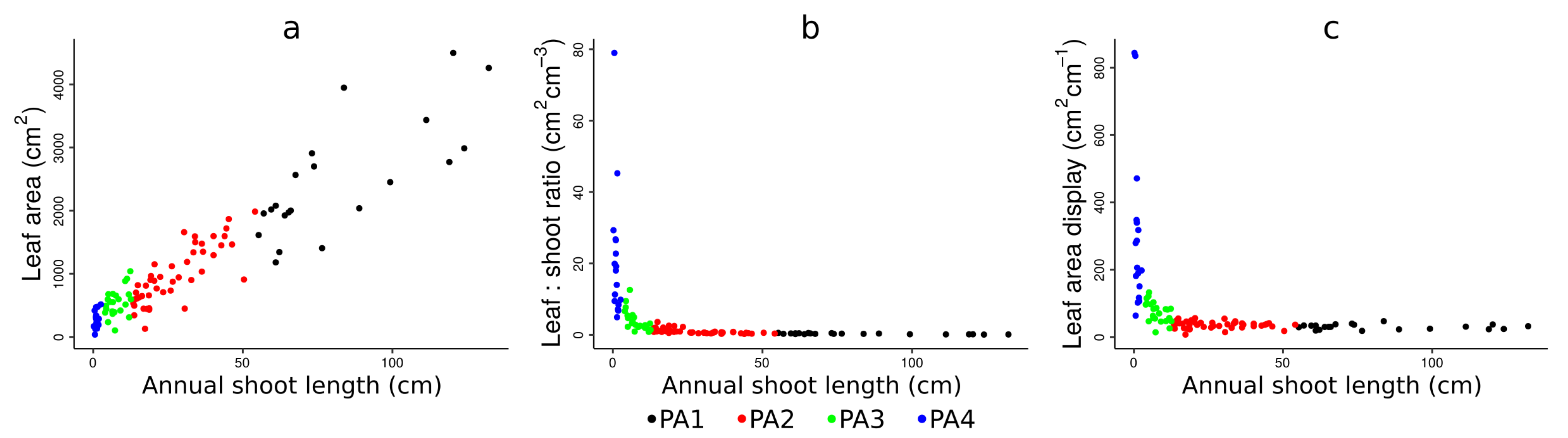
4.1. Physiological Ages Partitioning and Functional Attributes

As in previous findings, in this study, the AS leaf area (LA) positively correlates with the AS length (Kendall $\tau$ = 0.746) while both leaf area density (LAD) and the leaf-to-shoot ratio (L:S) correlates negatively to AS length ($\tau$ = −0.592 and $\tau$ = −0.809, respectively) and follow a negative exponential trend (Figure 8 [2,3]). These results show that, as expected, the morphological and functional variables correlate with the AS length and, therefore, that achieving PA partitioning based on AS length distribution would enable us to retrieve physiological ages with different functional attributes.

The distribution mixture model (DMM) that was used to retrieve the PAs from AS length distribution fits the data adequately (${\chi }^2$ test’s p = 0.411, Figure 9). The retrieved distributions parameters are summarized in Table 1. Based on this DMM, length thresholds separating two different PAs are set as the length corresponding to the fitted distributions intersection (Figure 9, Table 1).

The ASs classified using the DMM model present statistically significant differences in terms of LA, LAD, and L:S (The pairwise comparisons achieved using a Kruskal–Wallis test are summarized in

Table 2. Morphological and functional variables as a function of the four annual shoot physiological ages (PA) created with the distribution mixture model. The groups (gr) correspond to pairwise comparisons using the Kruskal–Wallis test with ($\alpha$ = 0.05).

	LA (cm${}^2$)		LAD (cm${}^2$.cm${}^{-1}$)		L:S (cm${}^2$.cm${}^{-3}$)
	Mean (±sd)	gr	Mean (±sd)	gr	Mean (±sd)	gr
PA1	2478 (±933.25)	a	30.39 (±7.34)	d	0.28 (±0.14)	d
PA2	973.76 (±453.39)	b	37.55 (±12.46)	c	1.02 (±0.73)	c
PA3	537.26 (±222.44)	c	73.85 (±30.95)	b	3.99 (±2.95)	b
PA4	271.76 (±136.70)	d	296.17 (±230.60)	a	21.06 (±18.22)	a

.): LA decreases with increasing PA order, and the reverse trend was observed for LAD and L:S (Figure 8).

These results show that DMM models are able to create PAs with contrasted morphological and functional properties. As expected, PA1 corresponds to long axialized shoots mostly specialized in space exploration as it exhibits a low investment in leaves relative to woody structure (low L:S) but still supports a large leaf area (large LA) although foliage is not displayed efficiently (low LAD). Conversely, PA4 corresponds to short foliated shoots mostly specialized in space exploitation thanks to a high relative investment in leaves (high L:S) and efficient foliage display (high LAD) although it supports a relatively small LA. Both PA2 and PA3 present intermediate levels of specialization (Table 2, Figure 8).

The AS properties for these four PAs were used to calibrate the AmapSim model (see Supplementary Materials S1).

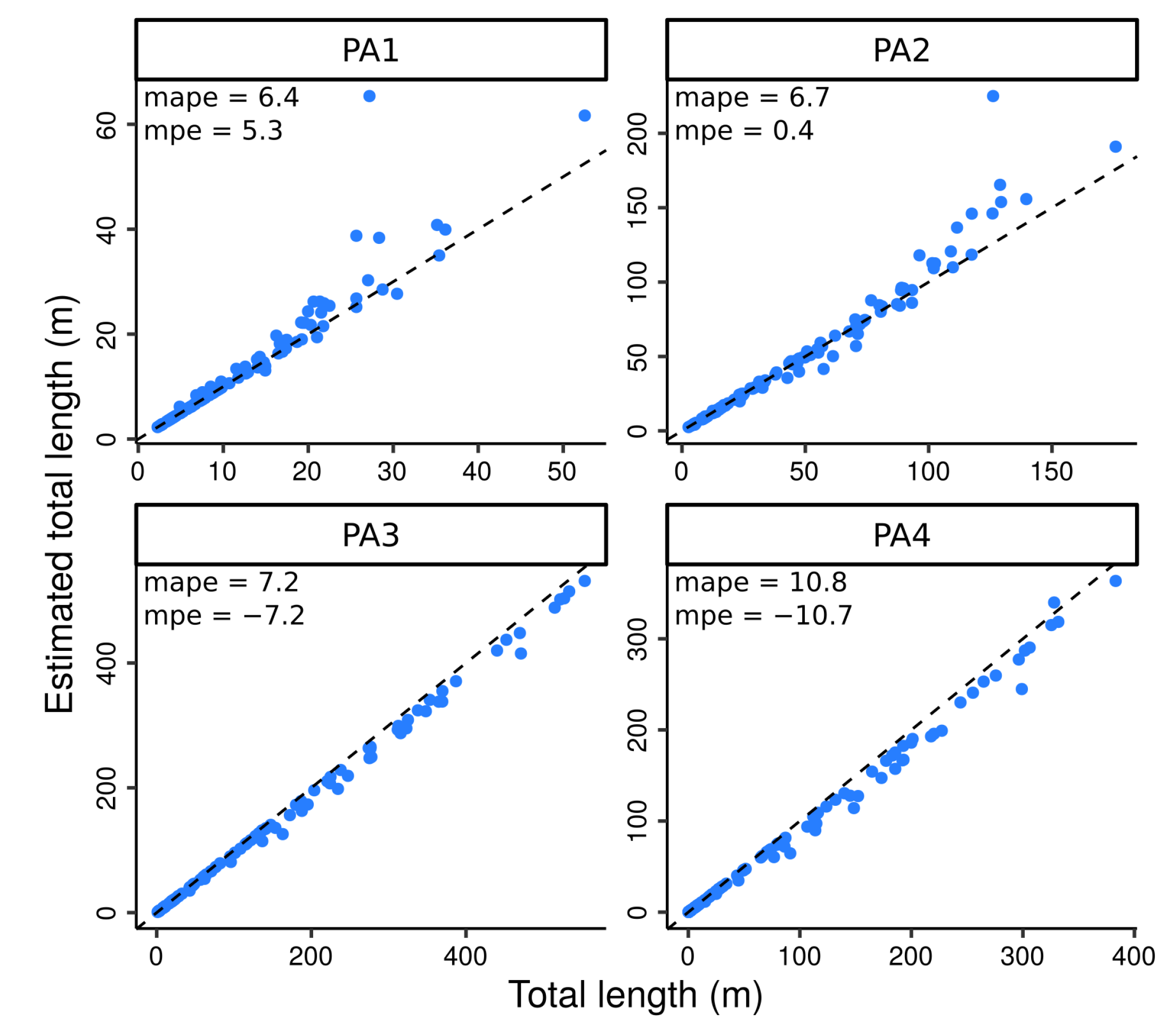
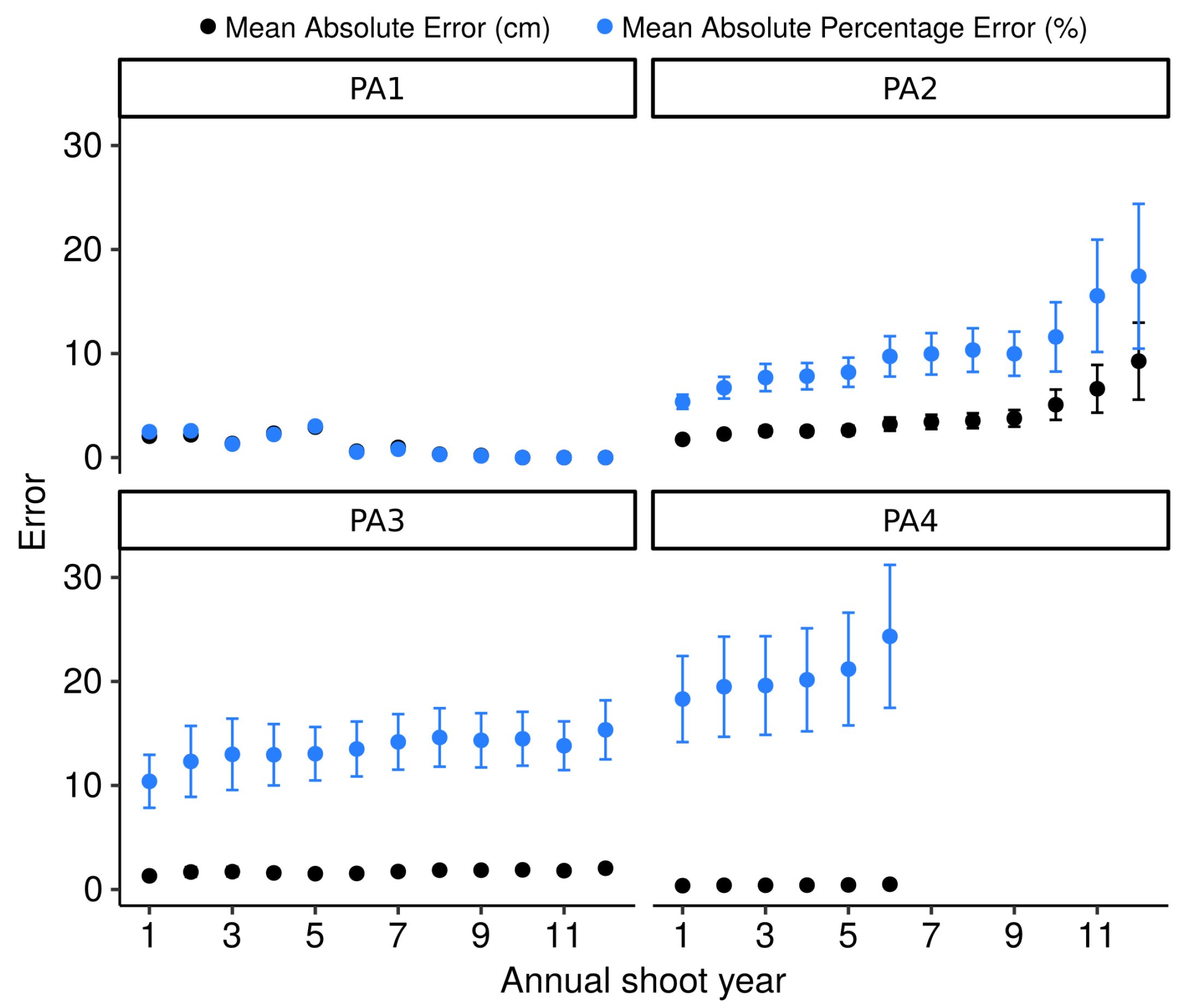
4.2. Testing the Algorithm against Perfect Data

Perfect tree skeletons were generated directly from the output file of the AMAPsim model, and the ASs segmented from the skeleton were matched to the original AS (i.e., the simulated AS) based on the xyz coordinates of their segment tips (i.e., the coordinates of the internodes).

Among all the trees, the annual shoot production year was correctly estimated in 90.85% of annual shoots and was comparable among physiological ages: 88.90% in PA1, 88.28% in PA2, 88.58% in PA3, and 91.62% in PA4. Annual shoot length prediction relative error increases with increasing PA order: mean absolute percentage error (mape) was 1.79% in PA1 (mean absolute error, mae = 1.67 cm), 6.6% in PA2 (mae = 2.57 cm), 10.43% in PA3 (mae = 1.55 cm), and 16.89% in PA4 (mae = 0.39 cm). This can be explained by the fact that PAs of higher order are less branched than those of lower order. Consequently, their annual shoots are segmented at the correction step (i.e., at step 6.4 in Figure 2) rather than by the acrotony-based model. Additionally, as the version of the annual shoot segmentation model dedicated to analyzing the perfect data is designed to arrange segments into annual shoots, the relative error increases with a decrease in the average number of internodes, i.e., with increasing PA order. This explains why the mean absolute prediction error equals the average internode length in PA3 and PA4. When summing the length of all annual shoots within one PA, the length of PA1 and PA2 were overestimated by 5.3% and 0.4%, respectively, while the length of PA3 and PA4 were underestimated by 7.2% and 10.7%, respectively (Figure 10).

In PA2, PA3, and PA4, the relative prediction error of annual shoot length tends to increase with increasing annual shoot production year (1 being the current annual shoot, Figure 11). This shows that AS segmentation errors might accumulate in the tree structure. However, these errors do not significantly affect PA classification of annual shoot as the overall classification success was 99.37%: 100% for PA1, 97.06% for PA2, 98.10% for PA3, and 99.82% for PA4. This indicates that the model is very effective for PA classification of AS.

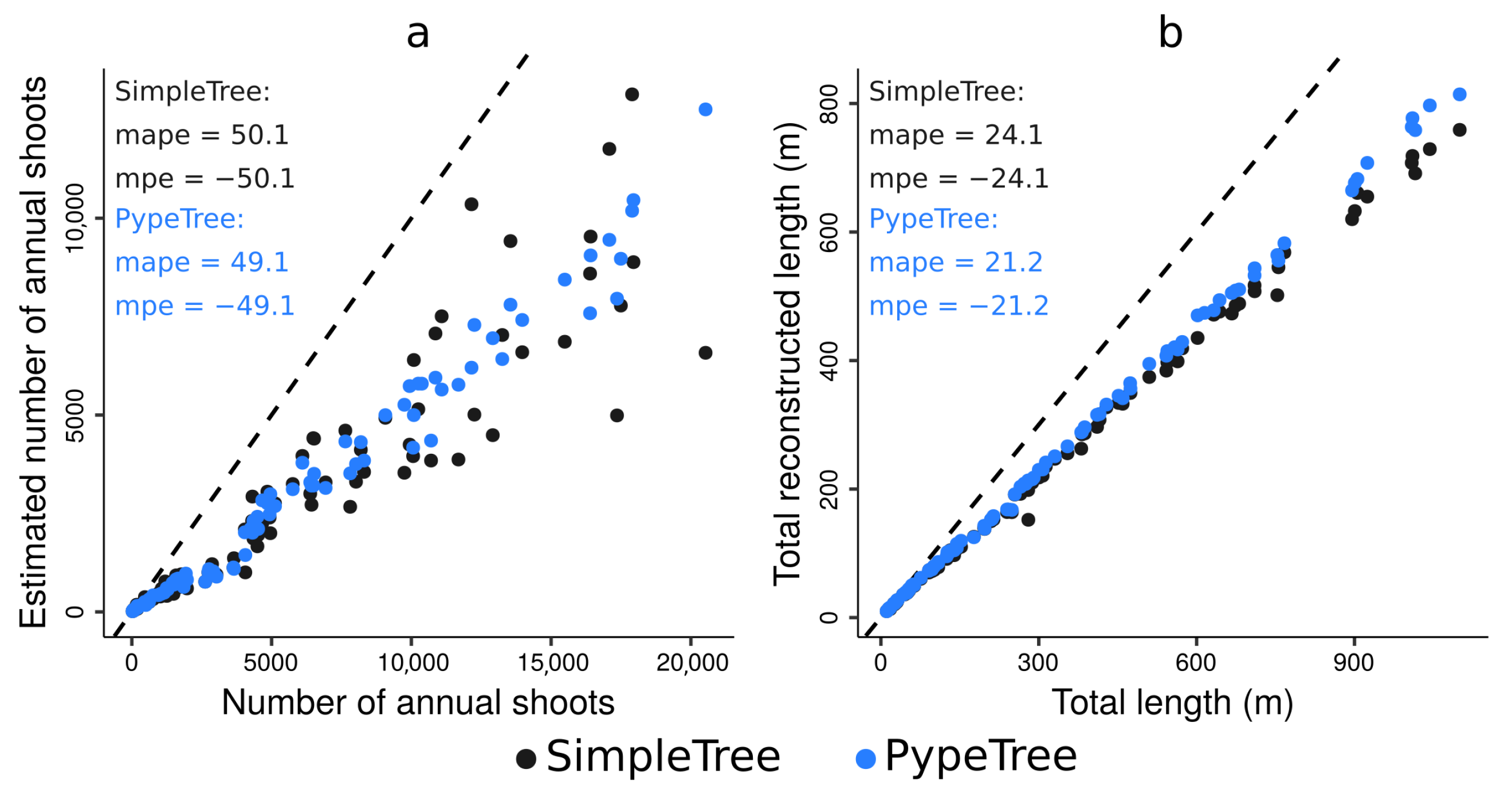
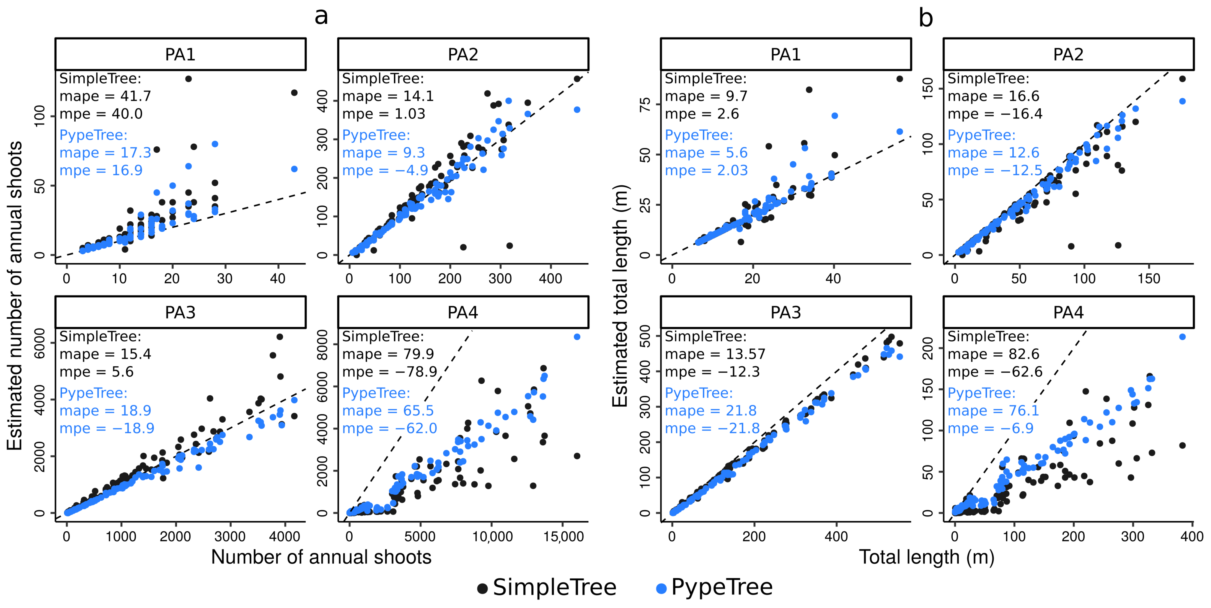
4.3. Testing the Algorithm against Skeletons Obtained from Simulated TLS Data

The two skeletonization models, i.e., PypeTree and SimpleTree, provide similar results as they enabled us to reconstruct 50.9% and 49.9%, respectively, of the total number of annual shoots (Figure 12a) and 78.8% and 75.1% of the overall tree length (Figure 12b), respectively. The proportion of reconstructed length and annual shoot number was lower than that obtained by Delagrange et al. [32], who found that, without manual work, 85% of the length and 58% of the axes of an elm tree (Ulmus americana L.) were reconstructed using the PypeTree model. These differences could be explained by the facts that (i) the elm tree used by Delagrange et al. [32] was small compared to the trees we simulated (2.5 m in height vs. 6.3 m to 20.7 m in our study) and (ii) the scanning conditions were optimal (Four scans were used for one single tree, while we used nine scans for ten trees,). According to this interpretation, we observed that >95% of the length and >76% of the number of annual shoots were reconstructed in 5–year-old trees while 70% to 75% of the length and 34% to 55% of the annual shoots were reconstructed in 10- to 15-year-old trees (data not shown).

These estimation errors are largely explained by a low detection rate of the small PA4 AS (that constitute a smaller proportion of the tree structure in young trees than in larger trees). The number of AS in PA4 was underestimated by 78.9% when the skeleton was extracted with SimpleTree and by 62.0% when the skeleton was extracted with PypeTree (mpe, Figure 13a), resulting in an underestimation of the total length of 62.8% and 6.9%, respectively (mpe, Figure 13b). Note, however, that the −6.9% mpe of the ST4 length obtained with PypeTree does not reflect the overall estimate goodness, as shown by the 76.1% mape (Figure 13b); this was due to an overestimation of PA4 length in some of the youngest trees.

When focusing on other PAs, the estimation errors were lower in both models in terms of AS number and total length. Both SimpleTree and PypeTree overestimated the total number (by 40.0% and 16.9%, respectively) and length (by 2.6% and 2.03%, respectively) of PA1 annual shoots. SimpleTree overestimated the PA2 and PA3 annual shoot numbers by 1.03% and 5.6%, respectively, while PypeTree underestimates them by 4.9% and 18.9%, respectively (Figure 13a). However, both models underestimated PA2 and PA3 total length by 16.4% and 12.3%, respectively, for SimpleTree and by 12.5% and 21.8%, respectively, for PypeTree (Figure 13b).

These results show that both SimpleTree and PypeTree performed poorly at detecting PA4 AS. Our results are similar to those obtained by Delagrange et al. [32], who found that only 26.0% of total number and 26.1% of total length of short axes were detected when applying PypeTree to a small elm tree. However, consistent with the Delagrange et al.’s study [32], the structural axes (i.e., PA1, PA2, and PA3) were detected with greater success than PA4. This suggests that the segmented tree skeletons are of sufficient quality to support an architectural automaton to add non-reconstructed axes to the skeleton.

A simple architectural automaton was used to model non-reconstructed PA4 and to add it to the reconstructed structure. The addition of non-reconstructed PA4 improved the estimated number of PA4 annual shoots from an underestimation of 78.9% to an overestimation of 10.7% in SimpleTree and from an underestimation of 62% to an overestimation of 9.8% when using PypeTree (mpe, compare Figure 14a to ST4 in Figure 13a). A similar improvement was observed for PA4 total length for the skeletons reconstructed using SimpleTree: from an underestimation of 62.6% to an overestimation of 0.6% (compare Figure 14b to ST4 in Figure 13b). However, these improvements were not valuable in skeletons reconstructed using PypeTree as the total PA4 length prediction error varied from an underestimation of 6.9% to an overestimation of 43.8%. When removing trees younger than 8 years of age from the analyses, i.e., trees for which the reconstructions were of lower quality, the average prediction error of PA4 length increased in skeletons obtained using SimpleTree (mae = 25.7% and mpe = −21%) but decreased in PypeTree (mae = 16.7% and mpe = 12.2%).

At the tree level, the addition of missing PA4 improved the estimates of both the total number of annual shoots (from −50.1% to 4.43% in SimpleTree and from −49.1% to −5.3% in PypeTree, Figure 14c) and total reconstructed length (from −24.1% to −12.2% in SimpleTree and from −21.2% to −11.5% in PypeTree, Figure 14d). These results show that using a simple architectural automaton to add the non-reconstructed axes might help to improve tree skeletonization quality. However, more complex modeling (e.g., with the addition of non-reconstructed ST3) could provide valuable additional improvements to the final skeleton.

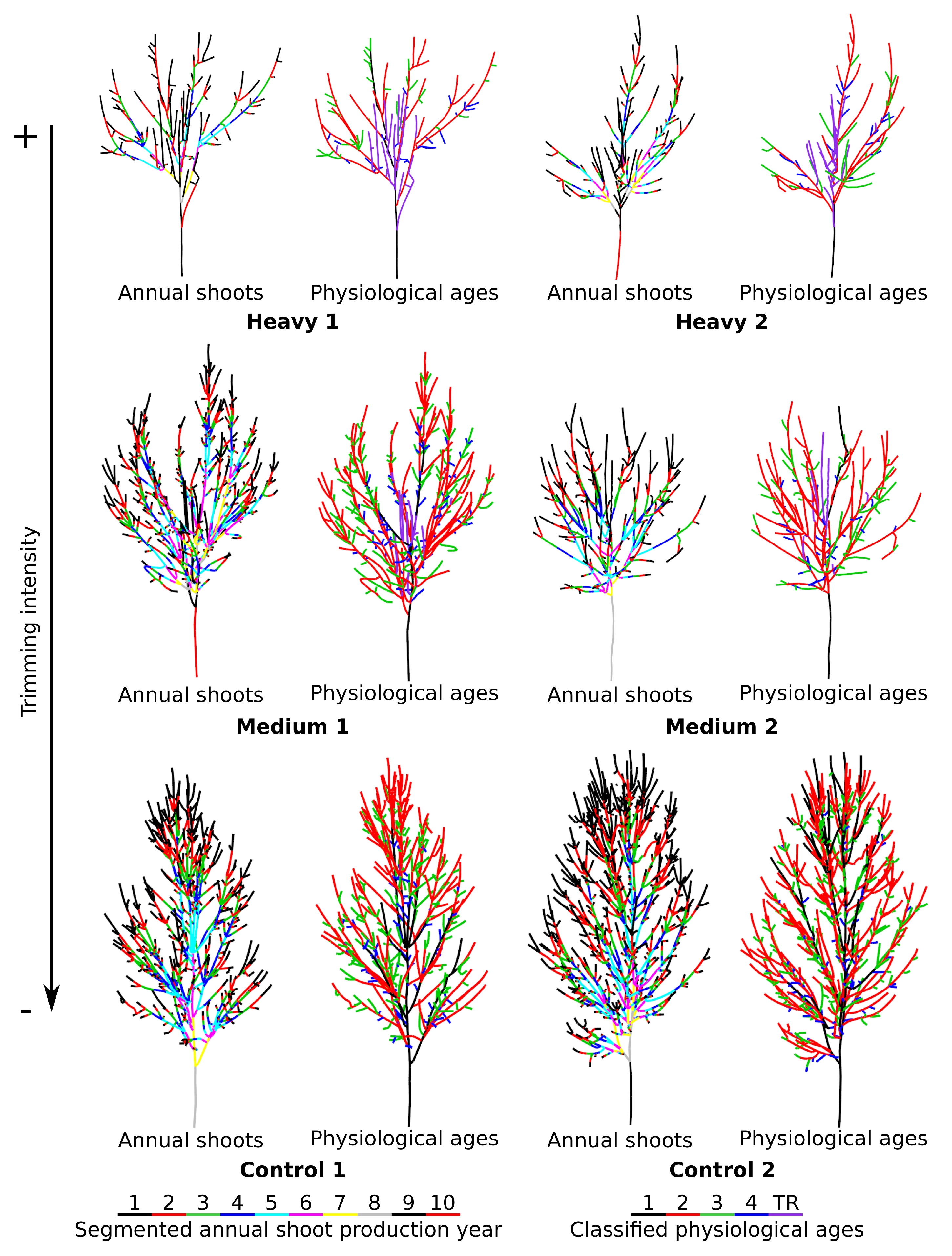
4.4. Real-Life Example

The annual shoot segmentation model was applied to six trees from a trimming experiment reconstructed using the SimpleTree model. The oldest annual shoot in the segmented tree structures were between 8 and 10 years old (Figure 15), which constitute a plausible result considering that the trees were 12 years old and that no annual shoot segmentation occurred on the trunk. We did not observe any pattern in difference in terms of estimated tree age between High intensity (H), Medium intensity (M), and Control (C) trees, suggesting that the annual shoot segmentation method is robust to the changes in tree form caused by trimming. Additionally, the position and size of the segmented TR were consistent with those observed in the field (Figure 15).

On average, the total reconstructed length was 76.8% lower in H trees and 43.5% in M trees relative to C trees. The total number of AS was reduced by 77.6% in H trees and by 34.5% in M trees relative to C trees.

When partitioning the reconstructed length and total number of annual shoots into physiological ages, PA1, PA2, PA3, and PA4 absolute total lengths decreased in the two trimming treatments relative to C trees (

Table 3. Length and annual shoot number in six red ashes from a tree trimming experiment. The total (number or length) as well as the total for each classified annual shoot types are presented (ST1 to 4 and traumatic reiterations, TR).

	Annual Shoot Length
	Total (m)	PA1 (m-%)	PA2 (m-%)	PA3 (m-%)	PA4 (m-%)	TR (m-%)
Heavy 1	42.02	3.72–8.89	17.26–40.08	6.78–16.14	4.19–9.97	10.07–23.96
Heavy 2	43.61	1.39–3.19	17.52–40.17	10.44–23.94	4.75–10.89	9.51–21.81
Medium 1	132.19	6.5–4.92	70.15–53.07	34.14–25.83	14.31–10.83	7.09–5.36
Medium 2	76.41	3.75–4.91	44.09–57.70	17.68–23.14	5.88–7.70	5.01–6.56
Control 1	153.76	18.73–12.18	76.28–49.61	45.06–29.31	13.69–8.90	-
Control 2	215.18	39.77–18.48	110.02–51.13	51.88–24.11	13.51–6.28	-
	Number of Annual Shoot
	Total (n)	PA1 (n-%)	PA2 (n-%)	PA3 (n-%)	PA4 (n-%)	TR (n-%)
Heavy 1	243	8–3.29	62–25.51	70–28.81	83–34.15	20–8.23
Heavy 2	288	1–0.35	74–25.69	94–32.64	94–32.64	25–8.68
Medium 1	1098	9–0.81	280–25.50	366–33.33	426–38.80	17–1.54
Medium 2	455	5–1.20	151–33.20	160–35.16	130–28.57	9–1.98
Control 1	1021	29–2.84	262–25.66	435–42.61	295–28.89	-
Control 2	1349	66–4.89	412–30.54	535–39.65	336–24.91	-

). However, only the proportion of total reconstructed length constituted by PA1 seems to decrease in both trimming treatments relative to C trees, while other PAs seem to remain relatively stable (Table 3). These results are consistent with the fact that trimming occurred on the tree trunk, also removing sequential reiterations that occurred when trees were around 10 years old.

The proportion and absolute value of both the total reconstructed length and number of annual shoots composed by traumatic reiterations (TR) were greater in H trees than in M trees while the average TR length was similar. Consistent with previous findings [57,58,59,60,61], this suggests that the more heavily a tree was trimmed, the more numerous the TR.

5. Discussion

5.1. Model Accuracy, Possible Applications, and Limitations

We developed a model that enables, for the first time, the segmentation of annual shoots (AS) from tree skeletons obtained using TLS data. The testing of this model against perfect data shows its strong efficiency for segment annual shoots (90% of detection success) and to provide good estimates of single AS length (error <3 cm in long shoots and <0.5 cm in short shoots). We also demonstrate that, by applying distribution mixture models (DMM) to the frequency distribution of annual shoot length, we are able to retrieve physiological ages (PA) of annual shoots that exhibit contrasted morphological and functional attributes. When combining the AS segmentation model and the PA classification of an AS, we successfully partitioned perfect skeletons into four PAs (classification success 99%).

On the other hand, when applying the model to simulated TLS data, the low detection rate of short axes by QSM models (PA4, only 20% to 38% of AS number and 20% to 25% of total length are adequately reconstructed) results in lower overall reconstruction quality (~50% of the annual shoots and 75% to 80% of the total tree length are reconstructed). However, the reconstructions obtained for longer axes (i.e., PA1, PA2, and PA3) remain relatively good (prediction error of the total length varies from 2.6% to −21.8% depending on the PA and QSM model considered), supporting the application of an architectural automaton of adding non-reconstructed PA4 axes. This could substantially improve the overall reconstructions, of the PA4 as well as the entire tree, suggesting that this workflow could help to improve the reconstruction quality of incomplete QSMs, which might be useful for a variety of applications.

This annual shoot segmentation model could be used to identify the current year AS to support the application of an algorithm dedicated to adding leaves to a reconstructed tree structure (e.g., [41]). Quantitative variables of ASs could also be derived, such as the number of internodes, the number of leaves, or the leaf area, through the application of allometric relations [39], making their application possible on large reconstructed tree structures. This method could also be used in plant phenotyping, which often consists of retrieving and quantifying the abundance of different structural elements [62] such as specialized axes [63,64]. However, quantifying the abundance of different axes types trough manual digitization is time consuming [65] and TLS has been mostly used to derive coarse variables of the tree canopy (e.g., crown volume and leaf area [66]). Therefore, the ability of our method to classify different elements of a tree structure into a finite number of features could help to improve, for example, the phenotyping of fruit trees where fruits are borne on specialized axes types. This method could also be used in fundamental research on tree architecture as the composition of a tree crown in terms of axes types express the state of functioning of the tree [1,5,63]. This method could also constitute a first step toward the combination of TLS-derived tree reconstruction and functional and structural tree models that often consider a finite set of structural elements as a building block [50,67]. Therefore, this method holds great potential in the study of tree structure and functions and could open the way to the developement of new approaches to analyze tree functions.

However, the present method can be limited by three aspects:

• the quality of the TLS point cloud that depends on scanning conditions and/or scanner technical characteristics (variations in point density, occlusion, noise caused by wind or “mixed pixel effect”, point deviation from the object surface, and low detection rate of small objects [28,68]);
• the capacity of the QSM and skeletonization methods to capture all the finest details of the point cloud; and
• the stage of development that influences the branching pattern, especially due to the drift effect [1]. This would limit the applicability of this method to large trees that do not express acrotony anymore.

Limitation 1 can be partly tackled by setting experiments on relatively small trees, in an open environment, during the leaf-off period, during days with no wind, by increasing the number of TLS stations around a given tree, and by placing the scanner close to the target tree. This will help to reduce occlusion without increasing point cloud noise as well as increasing small objects detection rates. In addition, using noise filtering will help to improve scan quality by reducing the influence of the “mixed pixel effect”. However, one should acknowledge that TLS have inherent limitations [68] and that, even when applying all the previous recommendations, TLS point clouds still does not represent a perfect image of a tree. QSM and skeletonization methods are a very active field of research, and one can expect that the development of new methods will help to reduce limitation 2. At this time, modeling approaches can be used to reconstruct the missing portions of the tree structure. Limitation 3 could be tackled trough the use of more complex segmentation methods (e.g., by using statistical models), but more work is needed to develop such methods. In its current form and considering the state-of-the-art in QSM and skeletinization methods, we thus believe that the annual shoot segmentation model should be used in a context where scans of very high quality are available and should be restricted to small to medium trees that are still in a base effect or acrotony stage of development [1].

5.2. On the Use of Distribution Mixture Models to Retrieve Annual Shoot Physiological Ages

We demonstrate that distribution mixture models (DMM) are a promising tool for recognizing PAs based on very simple measurements of the tree architecture (i.e., measuring only AS length) and botanical knowledge (the number of different PAs that can occur). The annual shoots classified using a DMM present morphological and functional differences that reflect well the morphogenic gradient that exists among tree axes [1,5]. Using only the AS length also greatly reduces data collection in the field and, therefore, eases application of the model and study replication. However, abiotic effects such as the climate could influence annual shoot length through their influence on organogenesis and growth. Therefore, more complex models, such as Markov-chain-based models [69] may help in obtaining annual shoot physiological ages along temporal variations. Additionally, it is unclear how DMM will work for other species that may exhibit less contrasted physiological ages than red ash.

5.3. Toward a More Complex Model

In its present form, the hypothesis on which the AS segmentation model relies limits its applicability to species with strong acrotony and trees that do not exhibit a high prevalence of immediate branching. Therefore, our method is best suited for trees growing in optimal conditions so that they are able to express their full developmental potential and to express more clearly their architectural model [1] which is the case for the red ashes growing in the open that were used in the “real life” example. To accommodate a wider range of cases, some parts of the model’s workflow could be replaced by more robust statistical approaches. For example, statistical models based on Markov chains are shown to be very efficient at retrieving patterns in trees architecture [70,71]. Such models could be used at the annual shoot segmentation step to more efficiently segment annual shoots or at the segmentation correction step to detect inconsistent patterns in the segmented annual shoots.

References

1. Barthélémy, D.; Caraglio, Y. Plant Architecture: A Dynamic, Multilevel and Comprehensive Approach to Plant Form, Structure and Ontogeny. Ann. Bot. 2007, 99, 375–407. [Google Scholar] [CrossRef] [PubMed] [Green Version]
2. Yagi, T.; Kikuzawa, K. Patterns in Size-Related Variations in Current-Year Shoot Structure in Eight Deciduous Tree Species. J. Plant Res. 1999, 112, 343–352. [Google Scholar] [CrossRef]
3. Yagi, T. Morphology and Biomass Allocation of Current-Year Shoots of Ten Tall Tree Species in Cool Temperate Japan. J. Plant Res. 2000, 113, 171–183. [Google Scholar] [CrossRef]
4. Puntieri, J.; Torres, C.; Magnin, A.; Stecconi, M.; Grosfeld, J. Structural Differentiation among Annual Shoots as Related to Growth Dynamics in Luma Apiculata Trees (Myrtaceae). Flora 2018, 249, 86–96. [Google Scholar] [CrossRef]
5. Taugourdeau, O.; Delagrange, S.; Lecigne, B.; Sousa-Silva, R.; Messier, C. Sugar Maple (Acer Saccharum Marsh.) Shoot Architecture Reveals Coordinated Ontogenetic Changes between Shoot Specialization and Branching Pattern. Trees 2019, 33, 1615–1625. [Google Scholar] [CrossRef]
6. Fernández-Sarría, A.; Martínez, L.; Velázquez-Martí, B.; Sajdak, M.; Estornell, J.; Recio, J.A. Different Methodologies for Calculating Crown Volumes of Platanus Hispanica Trees Using Terrestrial Laser Scanner and a Comparison with Classical Dendrometric Measurements. Comput. Electron. Agric. 2013, 90, 176–185. [Google Scholar] [CrossRef]
7. Bayer, D.; Reischl, A.; Rötzer, T.; Pretzsch, H. Structural Response of Black Locust (Robinia Pseudoacacia L.) and Small-Leaved Lime (Tilia Cordata Mill.) to Varying Urban Environments Analyzed by Terrestrial Laser Scanning: Implications for Ecological Functions and Services. Urban For. Urban Green. 2018, 35, 129–138. [Google Scholar] [CrossRef]
8. Hackenberg, J.; Wassenberg, M.; Spiecker, H.; Sun, D. Non Destructive Method for Biomass Prediction Combining TLS Derived Tree Volume and Wood Density. Forests 2015, 6, 1274–1300. [Google Scholar] [CrossRef]
9. Paynter, I.; Genest, D.; Peri, F.; Schaaf, C. Bounding Uncertainty in Volumetric Geometric Models for Terrestrial Lidar Observations of Ecosystems. Interface Focus 2018, 8, 20170043. [Google Scholar] [CrossRef] [PubMed] [Green Version]
10. Lau, A.; Bentley, L.P.; Martius, C.; Shenkin, A.; Bartholomeus, H.; Raumonen, P.; Malhi, Y.; Jackson, T.; Herold, M. Quantifying Branch Architecture of Tropical Trees Using Terrestrial LiDAR and 3D Modelling. Trees 2018, 32, 1219–1231. [Google Scholar] [CrossRef] [Green Version]
11. Owers, C.J.; Rogers, K.; Woodroffe, C.D. Terrestrial Laser Scanning to Quantify Above-Ground Biomass of Structurally Complex Coastal Wetland Vegetation. Estuar. Coast. Shelf Sci. 2018, 204, 164–176. [Google Scholar] [CrossRef] [Green Version]
12. Stovall, A.E.L.; Anderson-Teixeira, K.J.; Shugart, H.H. Assessing Terrestrial Laser Scanning for Developing Non-Destructive Biomass Allometry. For. Ecol. Manag. 2018, 427, 217–229. [Google Scholar] [CrossRef]
13. Fan, G.; Nan, L.; Dong, Y.; Su, X.; Chen, F. AdQSM: A New Method for Estimating Above-Ground Biomass from TLS Point Clouds. Remote Sens. 2020, 12, 3089. [Google Scholar] [CrossRef]
14. Nock, C.A.; Lecigne, B.; Taugourdeau, O.; Greene, D.F.; Dauzat, J.; Delagrange, S.; Messier, C. Linking Ice Accretion and Crown Structure: Towards a Model of the Effect of Freezing Rain on Tree Canopies. Ann. Bot. 2016, 117, 1163–1173. [Google Scholar] [CrossRef] [Green Version]
15. Martin-Ducup, O.; Robert, S.; Fournier, R.A. Response of Sugar Maple (Acer Saccharum, Marsh.) Tree Crown Structure to Competition in Pure versus Mixed Stands. For. Ecol. Manag. 2016, 374, 20–32. [Google Scholar] [CrossRef]
16. Lecigne, B.; Delagrange, S.; Messier, C. Exploring Trees in Three Dimensions: VoxR, a Novel Voxel-Based R Package Dedicated to Analysing the Complex Arrangement of Tree Crowns. Ann. Bot. 2018, 121, 589–601. [Google Scholar] [CrossRef]
17. Malhi, Y.; Jackson, T.; Patrick Bentley, L.; Lau, A.; Shenkin, A.; Herold, M.; Calders, K.; Bartholomeus, H.; Disney, M.I. New Perspectives on the Ecology of Tree Structure and Tree Communities through Terrestrial Laser Scanning. Interface Focus 2018, 8, 20170052. [Google Scholar] [CrossRef] [Green Version]
18. Hosoi, F.; Omasa, K. Voxel-Based 3-D Modeling of Individual Trees for Estimating Leaf Area Density Using High-Resolution Portable Scanning Lidar. IEEE Trans. Geosci. Remote Sens. 2006, 44, 3610–3618. [Google Scholar] [CrossRef]
19. Béland, M.; Widlowski, J.-L.; Fournier, R.A.; Côté, J.-F.; Verstraete, M.M. Estimating Leaf Area Distribution in Savanna Trees from Terrestrial LiDAR Measurements. Agric. For. Meteorol. 2011, 151, 1252–1266. [Google Scholar] [CrossRef]
20. Béland, M.; Widlowski, J.-L.; Fournier, R.A. A Model for Deriving Voxel-Level Tree Leaf Area Density Estimates from Ground-Based LiDAR. Environ. Model. Softw. 2014, 51, 184–189. [Google Scholar] [CrossRef]
21. Li, S.; Dai, L.; Wang, H.; Wang, Y.; He, Z.; Lin, S. Estimating Leaf Area Density of Individual Trees Using the Point Cloud Segmentation of Terrestrial LiDAR Data and a Voxel-Based Model. Remote Sens. 2017, 9, 1202. [Google Scholar] [CrossRef] [Green Version]
22. Xie, D.; Wang, X.; Qi, J.; Chen, Y.; Mu, X.; Zhang, W.; Yan, G. Reconstruction of Single Tree with Leaves Based on Terrestrial LiDAR Point Cloud Data. Remote Sens. 2018, 10, 686. [Google Scholar] [CrossRef] [Green Version]
23. Magney, T.S.; Eitel, J.U.H.; Griffin, K.L.; Boelman, N.T.; Greaves, H.E.; Prager, C.M.; Logan, B.A.; Zheng, G.; Ma, L.; Fortin, E.A.; et al. LiDAR Canopy Radiation Model Reveals Patterns of Photosynthetic Partitioning in an Arctic Shrub. Agric. For. Meteorol. 2016, 221, 78–93. [Google Scholar] [CrossRef]
24. Li, W.; Guo, Q.; Tao, S.; Su, Y. VBRT: A Novel Voxel-Based Radiative Transfer Model for Heterogeneous Three-Dimensional Forest Scenes. Remote Sens. Environ. 2018, 206, 318–335. [Google Scholar] [CrossRef]
25. Seidel, D. A Holistic Approach to Determine Tree Structural Complexity Based on Laser Scanning Data and Fractal Analysis. Ecol. Evol. 2018, 8, 128–134. [Google Scholar] [CrossRef]
26. Martin-Ducup, O.; Ploton, P.; Barbier, N.; Momo Takoudjou, S.; Mofack, G.; Kamdem, N.G.; Fourcaud, T.; Sonké, B.; Couteron, P.; Pélissier, R. Terrestrial Laser Scanning Reveals Convergence of Tree Architecture with Increasingly Dominant Crown Canopy Position. Funct. Ecol. 2020, 34, 2442–2452. [Google Scholar] [CrossRef]
27. Verroust, A.; Lazarus, F. Extracting Skeletal Curves from 3D Scattered Data. In Proceedings of the Shape Modeling International ’99. International Conference on Shape Modeling and Applications, Aizu-Wakamatsu, Japan, 1–4 March 1999. [Google Scholar]
28. Bucksch, A.; Lindenbergh, R.; Menenti, M. SkelTre: Robust Skeleton Extraction from Imperfect Point Clouds. Vis. Comput. 2010, 26, 1283–1300. [Google Scholar] [CrossRef] [Green Version]
29. Bucksch, A.; Lindenbergh, R. CAMPINO—A Skeletonization Method for Point Cloud Processing. ISPRS J. Photogramm. Remote Sens. 2008, 63, 115–127. [Google Scholar] [CrossRef]
30. Li, R.; Bu, G.; Wang, P. An Automatic Tree Skeleton Extracting Method Based on Point Cloud of Terrestrial Laser Scanner. Int. J. Opt. 2017, 2017, 1–11. [Google Scholar] [CrossRef] [Green Version]
31. Raumonen, P.; Kaasalainen, M.; Åkerblom, M.; Kaasalainen, S.; Kaartinen, H.; Vastaranta, M.; Holopainen, M.; Disney, M.; Lewis, P. Fast Automatic Precision Tree Models from Terrestrial Laser Scanner Data. Remote Sens. 2013, 5, 491–520. [Google Scholar] [CrossRef] [Green Version]
32. Delagrange, S.; Jauvin, C.; Rochon, P. PypeTree: A Tool for Reconstructing Tree Perennial Tissues from Point Clouds. Sensors 2014, 14, 4271–4289. [Google Scholar] [CrossRef] [Green Version]
33. Hackenberg, J.; Spiecker, H.; Calders, K.; Disney, M.; Raumonen, P. SimpleTree—An Efficient Open Source Tool to Build Tree Models from TLS Clouds. Forests 2015, 6, 4245–4294. [Google Scholar] [CrossRef]
34. Du, S.; Lindenbergh, R.; Ledoux, H.; Stoter, J.; Nan, L. AdTree: Accurate, Detailed, and Automatic Modelling of Laser-Scanned Trees. Remote Sens. 2019, 11, 2074. [Google Scholar] [CrossRef] [Green Version]
35. Calders, K.; Newnham, G.; Burt, A.; Murphy, S.; Raumonen, P.; Herold, M.; Culvenor, D.; Avitabile, V.; Disney, M.; Armston, J.; et al. Nondestructive Estimates of Above-Ground Biomass Using Terrestrial Laser Scanning. Methods Ecol. Evol. 2015, 6, 198–208. [Google Scholar] [CrossRef]
36. Stovall, A.E.L.; Shugart, H.H. Improved Biomass Calibration and Validation with Terrestrial LiDAR: Implications for Future LiDAR and SAR Missions. IEEE J. Sel. Top. Appl. Earth Obs. Remote Sens. 2018, 11, 3527–3537. [Google Scholar] [CrossRef]
37. Disney, M.I.; Boni Vicari, M.; Burt, A.; Calders, K.; Lewis, S.L.; Raumonen, P.; Wilkes, P. Weighing Trees with Lasers: Advances, Challenges and Opportunities. Interface Focus 2018, 8, 20170048. [Google Scholar] [CrossRef] [PubMed] [Green Version]
38. Brede, B.; Calders, K.; Lau, A.; Raumonen, P.; Bartholomeus, H.M.; Herold, M.; Kooistra, L. Non-Destructive Tree Volume Estimation through Quantitative Structure Modelling: Comparing UAV Laser Scanning with Terrestrial LIDAR. Remote Sens. Environ. 2019, 233, 111355. [Google Scholar] [CrossRef]
39. Delagrange, S.; Rochon, P. Reconstruction and Analysis of a Deciduous Sapling Using Digital Photographs or Terrestrial-LiDAR Technology. Ann. Bot. 2011, 108, 991–1000. [Google Scholar] [CrossRef] [Green Version]
40. Qi, J.; Xie, D.; Zhang, W. Reconstruction of Individual Trees Based on LiDAR and in Situ Data. In Proceedings of the 2nd ISPRS International Conference on Computer Vision in Remote Sensing, Xiamen, China, 2 March 2016; Wang, C., Ji, R., Wen, C., Eds.; International Society for Optics and Photonics: Xiamen, China, 2016; p. 99011E. [Google Scholar]
41. Åkerblom, M.; Raumonen, P.; Casella, E.; Disney, M.I.; Danson, F.M.; Gaulton, R.; Schofield, L.A.; Kaasalainen, M. Non-Intersecting Leaf Insertion Algorithm for Tree Structure Models. Interface Focus 2018, 8, 20170045. [Google Scholar] [CrossRef]
42. Calders, K.; Origo, N.; Burt, A.; Disney, M.; Nightingale, J.; Raumonen, P.; Åkerblom, M.; Malhi, Y.; Lewis, P. Realistic Forest Stand Reconstruction from Terrestrial LiDAR for Radiative Transfer Modelling. Remote Sens. 2018, 10, 933. [Google Scholar] [CrossRef] [Green Version]
43. Murtagh, F.; Legendre, P. Ward’s Hierarchical Agglomerative Clustering Method: Which Algorithms Implement Ward’s Criterion? J. Classif. 2014, 31, 274–295. [Google Scholar] [CrossRef] [Green Version]
44. Murtagh, F.; Legendre, P. Ward’s Hierarchical Clustering Method: Clustering Criterion and Agglomerative Algorithm. arXiv 2011, arXiv:1111.6285. [Google Scholar]
45. R Core Team. Available online: https://www.r-project.org/ (accessed on 14 January 2021).
46. Millet, J. L’architecture des Arbres des réGions Tempérées, 1st ed.; MultiMondes: Montréal, QC, Canada, 2012; p. 397. [Google Scholar]
47. Perrette, G.; Delagrange, S.; Messier, C. Optimizing Reduction Pruning of Trees Under Electrical Lines: The Influence of Intensity and Season of Pruning on Epicormic Branch Growth and Wound Compartmentalization. Arboric. Urban For. 2020, 46, 432–449. [Google Scholar] [CrossRef]
48. Macdonald, P.; Du, J. mixdist: Finite Mixture Distribution Models. R Package. Available online: Https://CRAN.R-project.org/package=mixdist (accessed on 14 January 2021).
49. De Mendiburu, F. Agricolae: Statistical Procedures for Agricultural Researché. Available online: Https://CRAN.R-project.org/package=agricolae (accessed on 14 January 2021).
50. Barczi, J.-F.; Rey, H.; Caraglio, Y.; de Reffye, P.; Barthelemy, D.; Dong, Q.X.; Fourcaud, T. AmapSim: A Structural Whole-Plant Simulator Based on Botanical Knowledge and Designed to Host External Functional Models. Ann. Bot. 2007, 101, 1125–1138. [Google Scholar] [CrossRef] [PubMed] [Green Version]
51. Bechtold, S.; Höfle, B. Helios: A multi-purpose LiDAR simulation framework for research, planning and training of laser scanning operations with airborne, ground-based mobile and stationary platforms. ISPRS Ann. Photogramm. Remote Sens. Spat. Inf. Sci. 2016, 3, 161–168. [Google Scholar] [CrossRef] [Green Version]
52. Adler, D.; Murdoch, D.; Nenadic, O.; Urbanek, S.; Chen, M.; Gebhardt, A.; Bolker, B.; Csardi, G.; Strzelecki, A.; Senger, A.; et al. RGL: A R-Library for 3D Visualization with OpenGL. 11. R Package. Available online: Https://CRAN.R-project.org/package=rgl (accessed on 14 January 2021).
53. CloudCompare. Available online: https://www.danielgm.net/cc/ (accessed on 14 January 2021).
54. Hackenberg, J.; Morhart, C.; Sheppard, J.; Spiecker, H.; Disney, M. Highly Accurate Tree Models Derived from Terrestrial Laser Scan Data: A Method Description. Forests 2014, 5, 1069–1105. [Google Scholar] [CrossRef] [Green Version]
55. Computree. Available online: http://computree.onf.fr/?lang=en (accessed on 14 January 2021).
56. Faro. Available online: https://www.faro.com/ (accessed on 14 January 2021).
57. Deal, R.L. Development of Epicormic Sprouts in Sitka Spruce Following Thinning and Pruning in South-East Alaska. Forestry 2003, 76, 401–412. [Google Scholar] [CrossRef]
58. O’Hara, K.L.; York, R.A.; Heald, R.C. Effect of Pruning Severity and Timing of Treatment on Epicormic Sprout Development in Giant Sequoia. Forestry 2008, 81, 103–110. [Google Scholar] [CrossRef] [Green Version]
59. Attocchi, G. Effects of Pruning and Stand Density on the Productionof New Epicormic Shoots in Young Stands of Pedunculate Oak (Quercus robur L.). Ann. For. Sci. 2013, 70, 663–673. [Google Scholar] [CrossRef] [Green Version]
60. Maurin, V.; DesRochers, A. Physiological and Growth Responses to Pruning Season and Intensity of Hybrid Poplar. For. Ecol. Manag. 2013, 304, 399–406. [Google Scholar] [CrossRef]
61. Desrochers, A.; Maurin, V.; Tarroux, E. Production and Role of Epicormic Shoots in Pruned Hybrid Poplar: Effects of Clone, Pruning Season and Intensity. Ann. For. Sci. 2015, 72, 425–434. [Google Scholar] [CrossRef]
62. Li, Z.; Guo, R.; Li, M.; Chen, Y.; Li, G. A Review of Computer Vision Technologies for Plant Phenotyping. Comput. Electron. Agric. 2020, 176, 105672. [Google Scholar] [CrossRef]
63. Lauri, P.-E.; Kelner, J.-J. Shoot Type Demography and Dry Matter Partitioning: A Morphometric Approach in Apple (Malus x Domestica). Can. J. Bot. 2001, 79, 1270–1273. [Google Scholar] [CrossRef]
64. Stephan, J.; Sinoquet, H.; Dones, N.; Haddad, N.; Talhouk, S.; Lauri, P.-E. Light Interception and Partitioning between Shoots in Apple Cultivars Influenced by Training. Tree Physiol. 2008, 28, 331–342. [Google Scholar] [CrossRef] [Green Version]
65. Sinoquet, H.; Godin, C.; Rivet, P. Assessment of the Three-Dimensional Architecture of Walnut Trees Using Digitising. Silva Fenn. 1997, 31, 265–273. [Google Scholar] [CrossRef] [Green Version]
66. Colaço, A.F.; Molin, J.P.; Rosell-Polo, J.R.; Escolà, A. Application of Light Detection and Ranging and Ultrasonic Sensors to High-Throughput Phenotyping and Precision Horticulture: Current Status and Challenges. Hortic. Res. 2018, 5, 35. [Google Scholar] [CrossRef] [Green Version]
67. Cournède, P.-H.; Kang, M.-Z.; Mathieu, A.; Barczi, J.-F.; Yan, H.-P.; Hu, B.-G.; de Reffye, P. Structural Factorization of Plants to Compute Their Functional and Architectural Growth. Simulation 2006, 82, 427–438. [Google Scholar] [CrossRef]
68. Abegg, M.; Boesch, R.; Schaepman, M.E.; Morsdorf, F. Impact of Beam Diameter and Scanning Approach on Point Cloud Quality of Terrestrial Laser Scanning in Forests. IEEE Trans. Geosci. Remote Sens. 2020, 1–15. [Google Scholar] [CrossRef]
69. Taugourdeau, O.; Caraglio, Y.; Sabatier, S.; Guédon, Y. Characterizing the Respective Importance of Ontogeny and Environmental Constraints in Forest Tree Development Using Growth Phase Duration Distributions. Ecol. Model. 2015, 300, 61–72. [Google Scholar] [CrossRef]
70. GuéDon, Y.; BarthéLéMy, D.; Caraglio, Y.; Costes, E. Pattern Analysis in Branching and Axillary Flowering Sequences. J. Theor. Biol. 2001, 212, 481–520. [Google Scholar] [CrossRef]
71. Guédon, Y.; Caraglio, Y.; Heuret, P.; Lebarbier, E.; Meredieu, C. Analyzing Growth Components in Trees. J. Theor. Biol. 2007, 248, 418–447. [Google Scholar] [CrossRef] [PubMed]
Figure 1. Illustration of the differences between the botanical term (left) and the terms used to describe the skeleton components (right). On the left, = corresponds to the annual shoot delimitation.
Forests 12 00391 g001
Figure 5. A tree simulated with the AmapSim model at 8, 12, and 15 years of age. The arrows indicate the location of the reiteration that occurs at age 10.
Forests 12 00391 g005
Figure 6. Scenes, sampling plan, and simulated scans for a row of ten 13-year-old trees. The scene of the row, i.e., the mesh created from the mtg files, from above (a) and from the front (b). In (a,b), the TLS positions are represented by the purple diamonds except for one scan position for which the tripod and TLS device as well as its lateral viewing angle are shown. The resulting point clouds for the entire row (c) and the details for one tree (d) are shown after applying the statistical outliers filter.
Forests 12 00391 g006
Figure 7. Comparison between the skeletons of a 10-year-old simulated tree extracted using the PypeTree (left) and SimpleTree (right) models. The whole tree (top) and details of a branch (bottom) with the segments shown in black and grey.
Forests 12 00391 g007
Figure 8. Manual measurement of annual shoots leaf area ((a), τ = 0.746), leaf area:shoot volume ratio ((b), τ = −0.809) and leaf area display ((c), τ = −40.592) as a function of annual shoots length. The colours indicate the annual shoots’ physiological ages retrieved from the distribution mixture model (legend on the graph).
Forests 12 00391 g008
Figure 9. Distribution mixture of annual length to retrieve annual shoot physiological ages (PA). Four normal distributions (continuous curve) are fitted to the frequency distribution of annual shoot length (grey histograms) to build the distribution mixture model (dotted curve). The black triangles show the average value of each distribution, and the vertical lines show the position of intersections between two distributions used to retrieve PAs.
Forests 12 00391 g009
Figure 10. Total length of the annual shoots of each physiological age (PA) classified with the annual shoot segmentation model as a function of the the total length observed in the output file of the AMAPsim model for the corresponding PA; 110 trees were simulated at different ages ranging from 5 to 15 years (10 trees per age). The dotted line represent the 1:1 relation. The Mean Absolute Percentage Error (mape, %) and Mean Prediction Error (mpe) are indicated on the graphs.
Forests 12 00391 g010
Figure 11. Mean absolute error and mean absolute percentage error (±standard deviation) of individual annual shoot length segmented by the annual shoot segmentation model as a function of production year for each physiological age (PA). Note that the y axis scale is the same for both indicators and that annual shoot year = 1 corresponds to the current year annual shoot.
Forests 12 00391 g011
Figure 12. Evaluation of skeletonization and annual shoot segmentation in 110 simulated terrestrial laser scanning (TLS) scans of 110 simulated trees (5 to 15 years with 10 trees per age) reconstructed with two quantitative structural model (QSM) methods. Number of segmented annual shoot (a) and total reconstructed length (b) cumulated at the tree level. Evaluations were done against the real AS number and length observed in the output of the AMAPsim model. The dotted line represents the 1:1 relation. The Mean Absolute Percentage Error (mape, %) and Mean Percentage Error (mpe, %) are indicated on the graphs.
Forests 12 00391 g012
Figure 13. Evaluation of skeletonization and annual shoot segmentation in 110 simulated TLS scans of 110 simulated trees (5 to 15 years with 10 trees per age) reconstructed with two QSM methods. Number of segmented annual shoot (a) and total annual shoot length (b) in each physiological age (PA). Evaluations are done against the AS number and length observed in the output file of the AMAPsim model. The dotted line represents the 1:1 relation. The Mean Absolute Percentage Error (mape, %) and Mean Percentage Error (mpe, %) are indicated on the graphs.
Forests 12 00391 g013
Figure 14. Number and length of PA4 annual shoots and reconstructed total length after the addition of non-reconstructed PA4 using a simple architectural automaton. The number of annual shoot is evaluated for PA4 only (a) or for all PA at the tree level (c) as well as the total reconstructed length ((b,d), respectively). The Mean Absolute Percentage Error (mape, %) and Mean Percentage Error (mpe, %) are indicated on the graphs.
Forests 12 00391 g014
Figure 15. Skeletons of six red ashes from a trimming experiment obtained with the SimpleTree QSM model with segmented annual shoots (Segmented) and annual shoots classified into four physiological ages (Classified) using the parameters described in Table 1. In the classified annual shoot, TR (purple) corresponds to traumatic reiterations that occurred after tree trimming.
Forests 12 00391 g015