Article

Modelling Maritime Pine (Pinus pinaster Aiton) Spatial Distribution and Productivity in Portugal: Tools for Forest Management

by
Cristina Alegria
1,2,*,
Natália Roque
1,3,
Teresa Albuquerque
1,2,3,4,
Paulo Fernandez
1,5 and
Maria Margarida Ribeiro
1,2,6
1
Instituto Politécnico de Castelo Branco, 6000-084 Castelo Branco, Portugal
2
CERNAS-IPCB—Pólo de Castelo Branco do Centro de Estudos de Recursos Naturais, Ambiente e Sociedade, Unidade de Investigação e Desenvolvimento do Instituto Politécnico de Castelo Branco, 6000-084 Castelo Branco, Portugal
3
QRural—Qualidade de Vida no Mundo Rural, Unidade de Investigação e Desenvolvimento do Instituto Politécnico de Castelo Branco, 6000-084 Castelo Branco, Portugal
4
ICT—Instituto de Ciências da Terra, Universidade de Évora, 7000-849 Évora, Portugal
5
MED—Mediterranean Institute for Agriculture, Environment and Development, Universidade de Évora, 7006-554 Évora, Portugal
6
CEF—Forest Research Centre, School of Agriculture, University of Lisbon, Tapada da Ajuda, 1349-017 Lisbon, Portugal
*
Author to whom correspondence should be addressed.
Forests 2021, 12(3), 368; https://doi.org/10.3390/f12030368
Submission received: 2 March 2021 / Accepted: 14 March 2021 / Published: 19 March 2021
(This article belongs to the Special Issue Modelling and Managing the Dynamics of Pine Forests)

Abstract

:
Research Highlights: Modelling species’ distribution and productivity is key to support integrated landscape planning, species’ afforestation, and sustainable forest management. Background and Objectives: Maritime pine (Pinus pinaster Aiton) forests in Portugal were lately affected by wildfires and measures to overcome this situation are needed. The aims of this study were: (1) to model species’ spatial distribution and productivity using a machine learning (ML) regression approach to produce current species’ distribution and productivity maps; (2) to model the species’ spatial productivity using a stochastic sequential simulation approach to produce the species’ current productivity map; (3) to produce the species’ potential distribution map, by using a ML classification approach to define species’ ecological envelope thresholds; and (4) to identify present and future key factors for the species’ afforestation and management. Materials and Methods: Spatial land cover/land use data, inventory, and environmental data (climate, topography, and soil) were used in a coupled ML regression and stochastic sequential simulation approaches to model species’ current and potential distributions and productivity. Results: Maritime pine spatial distribution modelling by the ML approach provided 69% fitting efficiency, while species productivity modelling achieved only 43%. The species’ potential area covered 60% of the country’s area, where 78% of the species’ forest inventory plots (1995) were found. The change in the Maritime pine stands’ age structure observed in the last decades is causing the species’ recovery by natural regeneration to be at risk. Conclusions: The maps produced allow for best site identification for species afforestation, wood production regulation support, landscape planning considering species’ diversity, and fire hazard mitigation. These maps were obtained by modelling using environmental covariates, such as climate attributes, so their projection in future climate change scenarios can be performed.

1. Introduction

Nowadays, access to big spatial data on climate and other environmental variables has fostered the use of powerful techniques from artificial intelligence and spatial statistics, such as machine learning (ML) and geostatistical modeling, which, coupled with geographic information systems (GIS) allow for the construction of simulated maps for the species’ habitat suitability and productivity under the impacts of climate change [1,2,3,4,5,6,7,8,9,10,11].
Indeed, statistical modelling techniques such as classical regression (CR), generalized linear models (GLM), algorithmic modelling based on machine learning (ML), e.g., Bayesian networks (BNs), maximum entropy (MaxENT), and classification and regression trees (CART) have become increasingly popular [12]. For instance, some of these statistical modelling techniques were used to predict current and future suitable habitats and productivity for Maritime pine populations (Pinus pinaster Aiton) in Spain [1], the impact of climate change on the potential distribution of Mediterranean pines [2], and the current and future conflicts between Eucalypt plantations and high biodiversity areas in the Iberian Peninsula [3]. In Portugal, a bioclimatic modelling approach (MaxENT) was used to study the influence of environmental variables explaining the presence of strawberry tree (Arbutus unedo L.), a typically adapted species to the Mediterranean region, under climate change scenarios [4].
Regarding forest species’ productive potential mapping, several methodological approaches have been essayed in various studies [6,7,8,9,10,11]. In Portugal, forest species’ productive potential maps for present and future climate change scenarios are available, for each one of the seven forest management regions the country, as divided in [13]. Nevertheless, each of these regional maps were produced with different methodological approaches (e.g., using ecological–cultural characteristics and/or edaphic–climatic characteristics, or bioclimatic indices or productivity estimation), thus no consistency exists when considering the whole country.
Yet, in a recent study [11], current species’ potential maps were produced for Portugal using the species ecological envelopes methodology, proposed by DGRF (Direção Geral dos Recursos Florestais) [14], and afterwards, projected into the future under climate change scenarios. Moreover, in that study a Bayesian ML approach was used to explore the most influential environmental variables on current species’ distribution and productivity for the species essayed (Maritime pine and Eucalypt). The findings in that study indicated that the species’ ecological envelope methodology was robust and encouraged further investigation on fitting statistical ML models for the species’ distribution and productivity for Maritime pine in Portugal.
Maritime pine forests provide a significant amount of the wood harvested in Portugal [15] as raw material for the wood-based industry. According to the last National Forest Inventory (NFI 2015) this species’ forests area represents 23% of Portuguese forests (713 × 103 ha). However, the impact of climate change in Maritime pine forest area must not be neglected. Indeed, several studies have consistently reported a future decrease of potential areas of the Maritime pine, particularly in south of the Tagus river and the inland of Portugal, associated with a species’ migration trend from south to north and from the interior to coastal areas [11].
Maritime pine forests are mostly established by natural regeneration and managed in medium to long revolutions (e.g., more than 35 years) [15,16,17]. Maritime pine is a light pioneer species and viable seed production occurs later in stands of 15 to 20 years that ensures desirable natural regeneration [18].
In Portugal wildfires are currently a major issue and a serious challenge for forest management. In fact, during the 1950s and 1960s, the country observed a total burnt area of about 5000 ha year−1. Between 1975 and 1980, the total burnt area increased remarkably, reaching about 43,860 ha year−1. More recently, new historical values were attained in 2003, 2005 and 2015, respectively 425,839 ha, 339,089 ha, and 442,418 ha [19,20].
Undeniably, wildfires’ severity and recurrency, e.g., within a 10 to 15 year interval, have had a huge impact in Maritime pine forests, making the species’ post-fire recovery uncertain [21]. For instance, during the past decades Maritime pine’s post-fire area has been mainly converted into scrub, pastures, and Eucalypt plantations [19]. Moreover, forest owner’s confidence levels in sustaining Maritime pine management significantly dropped afterwards. In fact, a study in the central inland of Portugal noticed that these stands became less stable (inventory data 1991–1996 and 2007–2010) and under-stocked, with large amounts of small-diameter poles, and enlarged tree size variability, showing a decline in their management [22].
More recently, the industrial development of bioenergy production from biomass residues created another industrial destination for forests’ raw material which traditionally had no commercial value [23,24,25]. The opportunity to value forest residues resulting from silvicultural operations (e.g., brushing, cleaning, pruning, thinning, and harvesting) are an inducement to forest management and fire severity mitigation.
It is well known that fire hazard mitigation can be attained by a combination of different associated effects, such as forest type-appropriate management, together with stands’ age planification, density, and spatial landscape pattern arrangements (i.e., patch size, forest fragmentation) [26,27,28,29]. Indeed, what contributes most to fire severity are the species’ flammability and combustibility, spatial arrangement, vertical structure (high/low and close/open), and land topographic characteristics (slope and aspect) [27,28].
To that end, the definition of a forest type implies considering, among others, straightforward afforestation planning at the landscape level. The stand’s vertical structure can be managed through corresponding rearrangement by different ages, heights, or eligible density. The area control method by Davis and Johnson [30] allows for forest production regulation, introducing the age diversity factor to the landscape. Therefore, this method works as a tool on fire hazards mitigation by creating a stand age class progression (e.g., different succession stages) with different fuel loads, as well as vertical fuel continuities between harvesting compartments. Over time, the stands’ age class progression (e.g., different succession stages), due to their establishment and growth, results in a vertical structural change, from short and open (in the establishment phase), to short and close, and, eventually, tall and close (in the harvest phase). Finally, when the compartment is harvested (e.g., clear-cutting), a break in the fuel load is observed [26]. It is important to stress that application of the area control method requires previous knowledge of the area under productivity regulation [9,26]. Thus, the availability of cartographic support on species’ current and potential distributions and productivity is key as a supporting tool for integrated landscape planning, species’ afforestation, and sustainable forest management [26].
The present study focused on producing Maritime pine distribution and productivity maps by using a ML modelling approach. In a previous study [11], the authors used a predefined set of environmental variables to produce an ecological envelope map for the species’ potential distribution. Afterwards, a Bayesian ML approach highlighted that the species’ current distribution was mainly determined by precipitation-related variables, and that elevation- and temperature-related variables were very important to differentiate the species’ current productivity. However, these last variables were not the ones used to obtain the species’ ecological envelope map.
Therefore, in the current study, the research question was to verify if the set of environmental variables used in species’ ecological envelope map were also good regressors in the species’ distribution model (SDM) and species’ productivity model (SPM). Additionally, species’ spatial productivity modelling was also performed using an alternative methodological approach (sequential stochastic simulation). Hence, a full discussion about high and low Maritime pine’s productivity spots was made. Furthermore, the fitted species’ distribution model (SDM) and species’ productivity model (SPM) may be used to make projections of the future under climate change scenarios.
The specific aims of this study were: (1) firstly, to model the species’ spatial distribution and correspondent productivity using a ML Regression approach; (2) in a second step, to model the species’ spatial productivity through an alternative approach based on a sequential stochastic simulation process; (3) to produce a species’ potential distribution cartography and the definition of the ecological envelope’s thresholds by using a ML classification technique; and, finally (4) to identify present and future key factors of the species’ afforestation and optimized management. To that end, land cover and forest inventory, used as hard data, together with soft data attributes such as climate variables, topography, and soil information, were used to model species’ current and potential spatial distribution and productivity.

2. Materials and Methods
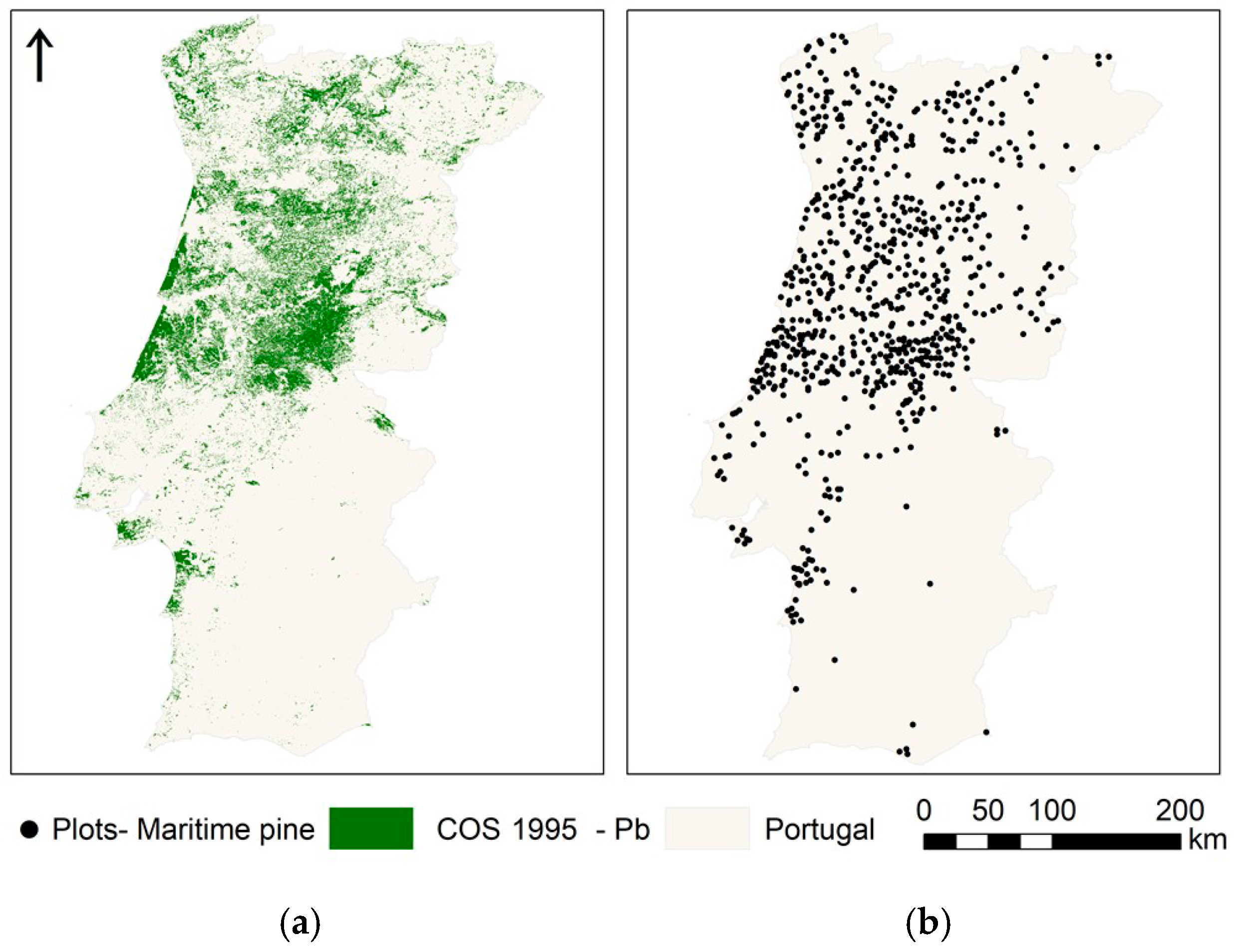
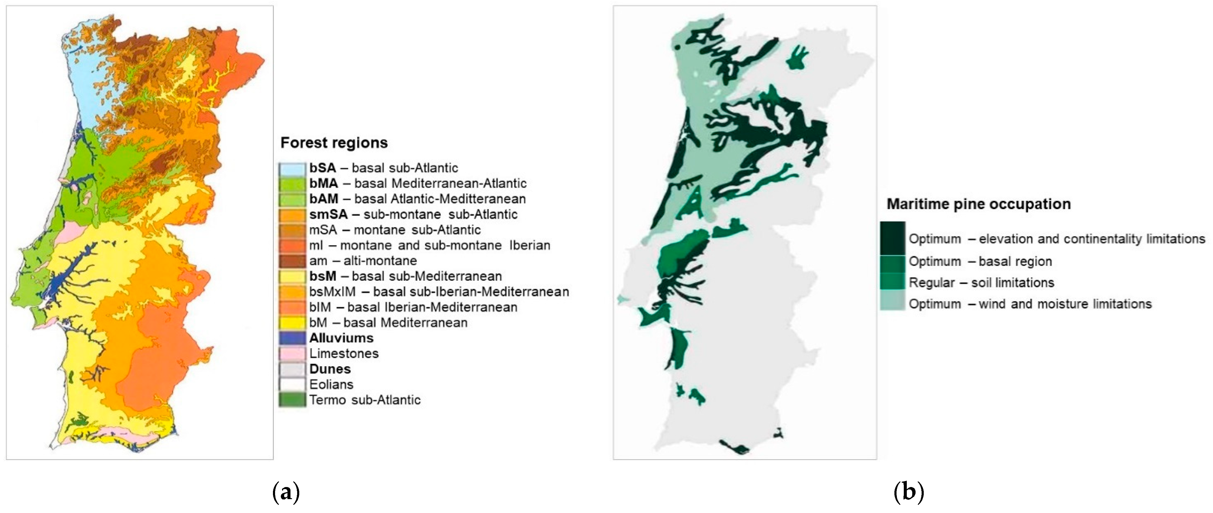
2.1. Study Area

The study area is Mainland Portugal (36.9636° N 9.4944° W and 42.1543° N 6.1892° W), located in the Iberian Peninsula (southwestern Europe), between Spain, to the east, and the Atlantic Ocean to the west. The annual temperature ranges from about 7 °C in the northern and central inland highlands to about 18 °C in the south coast. The average annual precipitation has the highest values in the north and northwest regions and the lowest values in the south and inland. The study area includes two climate classifications: (i) hot-summer Mediterranean in the south and central inland and lower elevations (below 800 m); and (ii) temperate Mediterranean in the north and northwest region of the country and higher elevations (above 800 m) [31].

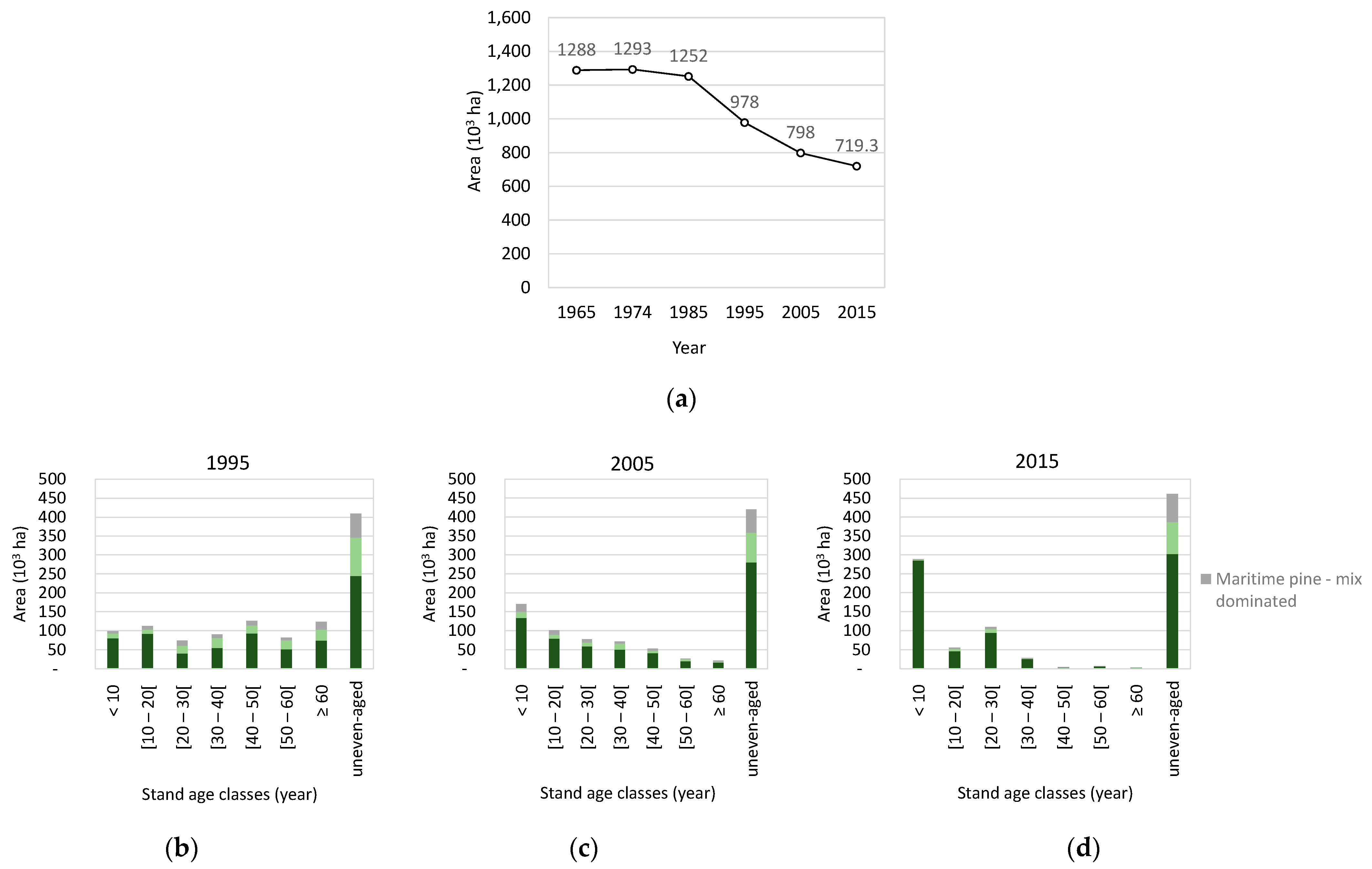
2.2. Hard Data—Land Cover and Forest Inventory

The Portuguese Land Cover and Land Use (LCLU) 1995 thematic map (COS1995) [32] was used to extract the Maritime pine’s forest cover layer. The COS1995 map has 1:25,000 scale, corresponding to the minimum cartographic unit of one ha. Furthermore, a five-level hierarchical classification with 89 classes segmentation at the most detailed level allowed a detailed analysis regarding this species’ forest cover (Figure 1). The COS1995 was available through the Web Feature Services (WFS) [33].
The National Forest Inventory 1995 was used to assess pure Maritime pine stands’ productivity, defined as forests where the dominant species represents more than 75% and the ground cover is higher than 10% [17,33,34] (Figure 1).

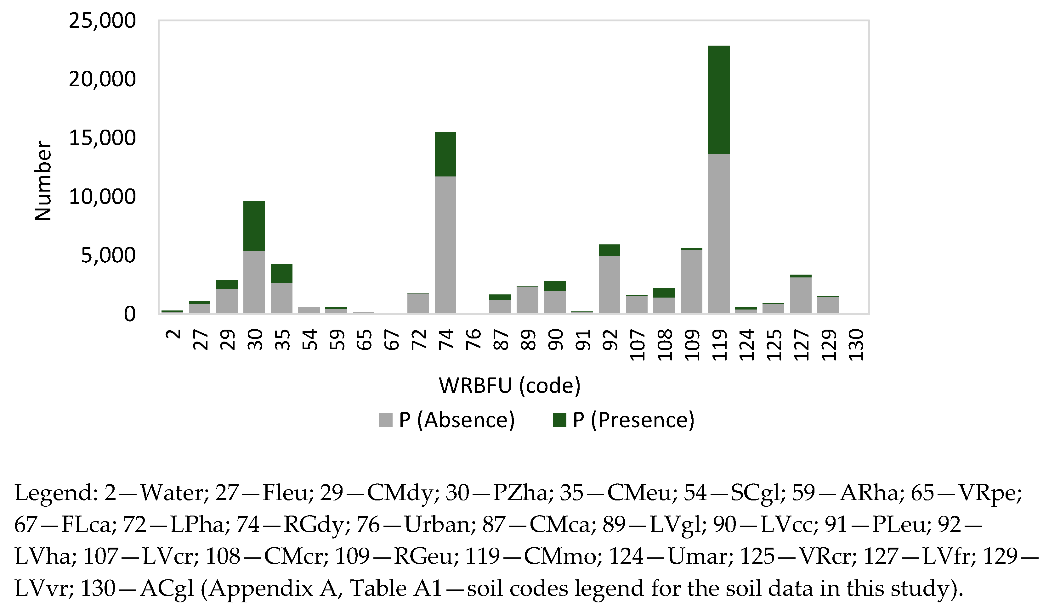
2.3. Soft Data—Climate, Topography, and Soil Attributtes

The climate data sets (Table 1) for the period between 1960 and 1990 was downloaded from the WorldClim site version 1.4, with a 1 km × 1 km grid [35]. The elevation data (Table 1) was derived from the Shuttle Radar Topography Mission 1 Arc-Second Global (SRTM1N22W016V3) with a spatial resolution of 30 m [36]. The soil data (Table 1) was derived from the ESDBv2 Raster Library in a 1 km × 1 km grid [37,38,39].
Climate variables (Table 1) followed the original WorldClim symbology, wherein the first variables from Tmax to BIO11 are temperature-related variables and variables from BIO12 to BIO19 are precipitation-related variables. The topographic-related variables considered were elevation, slope, and aspect. The soil-related variables used the soil codes according to the international classification system (Appendix A, Table A1—soil codes legend for the soil data in this study).

2.4. Methods

2.4.1. Species’ Distribution and Productivity Modeling—A Machine Learning Regression Approach

The species’ presence was extracted from COS1995 classes, in 1 km × 1 km grid, as a coverage percentage in each pixel (Pb95; species’ presence occurs when pixel percentage coverage is higher than 0). The same procedure was used for the correspondent bioclimatic attributes (1960–1990), topography and soil variables (Table 1).
To model the pure Maritime pine stands’ productivity, the site index was used, since it is the most widely accepted site productivity indicator [40]. The classical site index SI35 (i.e., the stand dominant height at the age of 35 years) fitted by Páscoa et al. [41] was evaluated for each inventory plot. It should be stressed that this site index model was fitted for the species and country using forest inventory data from 1995, as well. The extracted climate attributes, elevation, and soil data sets were projected in each plot location (Table 1).
WEKA (Waikato Environment for Knowledge Analysis) open-source software [42,43] was subsequently used for modelling purposes. WEKA allows for big data pre-processing, and the supported algorithms are organized under Classify, Cluster, Associate, and Select Attributes (SA). The SA was used as the regressor for covariates selection in the subsequent ML analysis.
The search method “Rankers” under the “Correlation Attribute Evaluation” provides a selection ranking technique for the predictors’ inclusion in the final regression model, by measuring the correlation (Pearson) between the predictor and the class. Thevalues were expressed in relative terms for comparability purposes, as follows:
RI = (rank−rankmin)/(rankmax−rankmin)
Afterwards, the seven best fitted variables were retained and used to model the species’ distribution (Pb95) and correspondent productivity (SI35). Additionally, a set of environmental variables were used for species’ ecological envelope delimitation, accordingly: BIO5, BIO6, BIO7, BIO12, E, WRBFU (Table 1).
ML models were fitted, under Classify, for the species’ distribution (Pb95; species’ presence occurs when pixel percentage coverage is higher than 0) and productivity (SI35). The variables Pb95 and SI35 are continuous variables, thus three ML regression trees algorithms were tested, namely: M5P, Random Forests (RF), and Random Tree (RT) [44,45]. WEKA software provides k-fold cross-validation to test the algorithm’s accuracy, by dividing the data set into k subsets. One of these subsets is randomly selected as the test set, and the other k-1 subset constitutes the training sample, in each run. The models’ fitting performance is assessed using statistics such as the pseudo-coefficient of determination (R2) [46], the mean absolute error (MAE) and the root mean squared error (RMSE). Under Classify, the species distribution (P; species presence and absence, that is P = 1 when Pb95 > 0 and P = 0 otherwise) was fitted. As the variable P is a discrete (nominal) variable, then three ML classification tree algorithms were tested, namely: J48, random forests (RF), and random tree (RT) [44,45]. Statistics such as Cohen’s kappa (kappa), MAE and RMSE statistics were computed for the models’ fitting performance assessments.

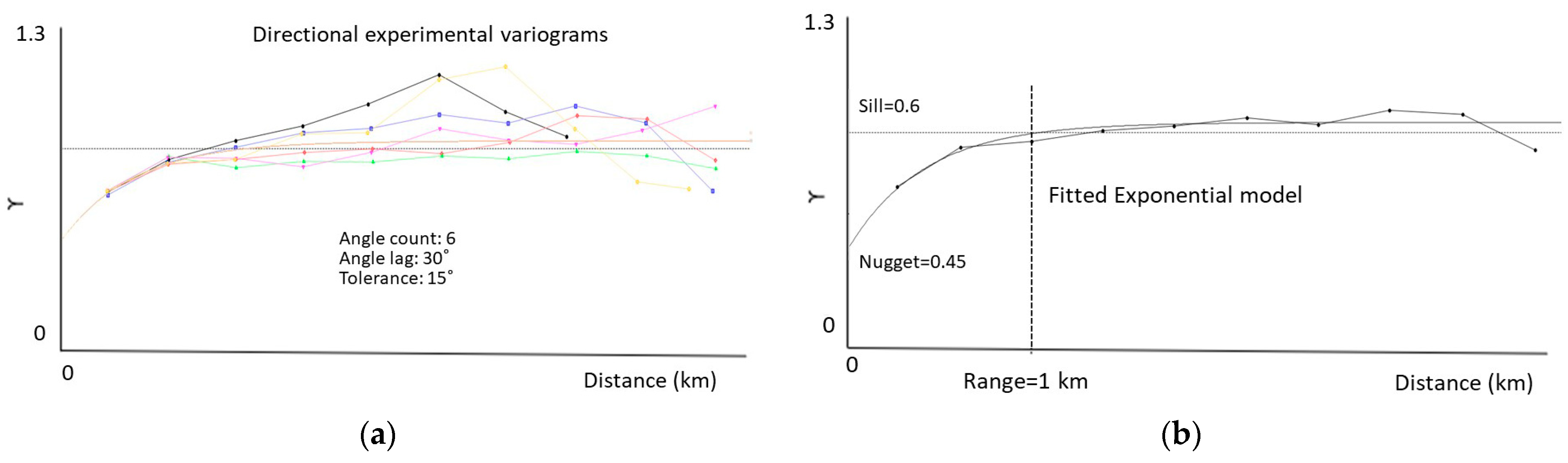
2.4.2. Species’ Productivity Modelling—A Sequential Gaussian Simulation Approach

The sequential Gaussian simulation (SGS), a stochastic sequential simulation algorithm, was used. This geostatistical approach starts with the definition of the univariate distribution normal scored values. Indeed, the first step is the normal score transformation of the measured values [47]. Furthermore, normal scores at 2 km × 2 km grid node locations were sequentially simulated using simple kriging (SK) with zero mean [48]. The SI35 spatial structure was performed through variography. Finally, the obtained outputs went through a back-transform function, allowing the results to be obtained in the original grade values. The Space-Stat software v.4.0.18 from Biomedware was used for computation purposes [48,49]. It is important to highlight that when multiple sequences of simulations are designed (100 different scenarios were performed), it is possible to obtain more accurate probabilistic maps. The mean image (MI) together with a representation of the spatial uncertainty (the 100 simulations standard deviation was used as the uncertainty measurement), allows the spatial productivity clusters robustness to be ascertained, and therefore constitutes a powerful tool for productivity evaluation and future management policies [11,50].

2.4.3. Species’ Ecological Envelope—Potential Distribution

The species’ potential distribution map was based on the methodology introduced by the DGRF (Direção Geral dos Recursos Florestais) [14] concerning the definition of the species’ ecological envelopes. Maritime pine’s ecological envelope is based on literature information [51] and was defined using the following five variables: (i) temperature range (T max Aug–T min Jan <26 °C); (ii) temperature limits (T max Aug <29.9 °C); (iii) precipitation (BIO12 > 850 mm); (iv) elevation (E < 800 m); and (v) lithology (different of limestone).
In this study, the variables’ threshold aimed to ensure that at least 75% of plots (1995), as the dominant species [33], are inside of the defined envelope. The soft covariates used for the species’ ecological envelope definition were selected through the ML regression tree algorithm J58. Additionally, to safeguard consistency in data usage in all produced maps, the soil data was used to set the lithology constraint as follows: WRFBU—soils differing by luvisols calcic, cambisols calcarean, and fluvisols calcic.
Afterward, the covariates’ thresholds were obtained fitting a ML classification tree model. The maps of the selected variables were constructed using the new thresholds and a subsequent Boolean reclassification (0—not suitable, 1—suitable). A map algebra approach was used for the species’ potential distribution map computation (i.e., the ecological envelope) as follows: ((BIO7 + (BIO6 × BIO5) + BIO12) × E × WRFBU). Finally, the final map was obtained, reclassifying into four suitability classes: 3—excellent (without temperature range, temperature limits, and precipitation restrictions), 2—good (with one restriction), 1—regular (with two restrictions), and 0—unsuitable (null).
The obtained map for the species’ potential distribution was then compared with the empirical maps for forest regions in Portugal by Alves et al. [52] and the Maritime pine occupation map by Oliveira [17] (Figure 2). The coverage of the Maritime pine plots in 1995 (Figure 1) was also assessed using its suitability class.

2.4.4. Species’ Afforestation and Management

The National Forest Inventory statistics (1968–2015) [15,16,53] were used to assess the Maritime pine forest changes in area and stand age structure through the years (1995–2005–2015) [15,16,54,55].
The maps produced in the study (current species distribution, species productivity, and species potential distribution) were evaluated together, aiming for an evaluation of the best sites for species settlement.

3. Results

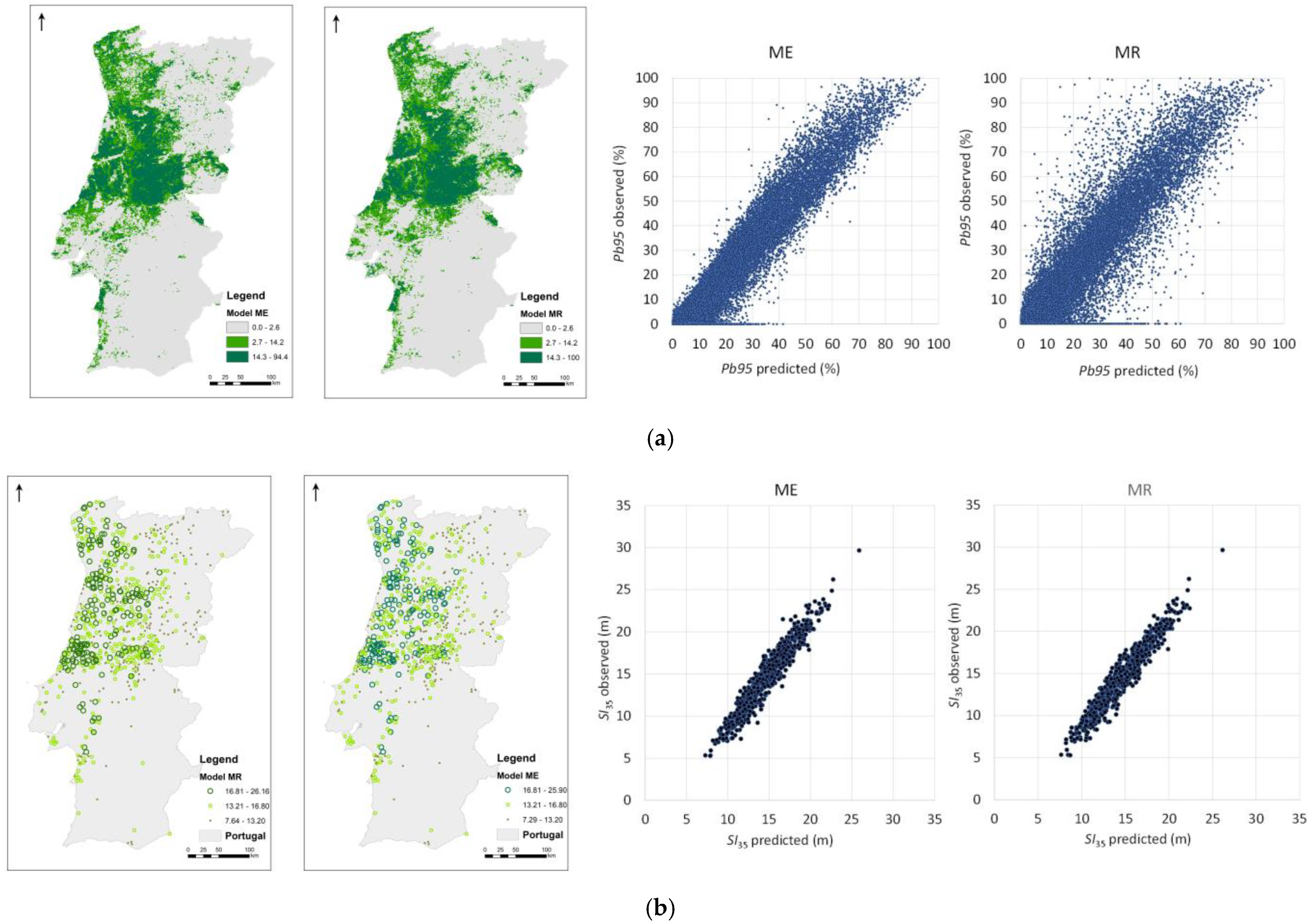
3.1. Species’ Distribution and Productivity Modelling—A Machine Learning Regression Approach

Two types of models (ME and MR) were used to predict species grid percentage coverage (Pb95), species presence (P), and site index (SI35) (Table 2). The ME models used as regressor variables were the same variables as the ecological envelope. The MR models used as regressor variables were the seven best variables selected by the search method “Rankers” according to their relative importance (RI; Table A2). It should be noted that all variables are continuous, with exception made to the variables P and WRBFU which are discrete (nominal variables). The relative importance (RI) of regressor variables for the Maritime pine distribution (Pb95) in the MR model was BIO13 > BIO19 > BIO16 > BIO12 > BIO18 > BIO17 > BIO2, and for Maritime pine presence (P) in the MR model, BIO7 > BIO16 > BIO4 > BIO19 > BIO13 > BIO12 > BIO2. For Maritime pine productivity (SI35) the ranking was BIO4 > BIO3 > E > BIO7 > BIO8 > BIO11 > BIO6.
The best performance was achieved by the “random forest” algorithm. The selected model for the species’ distribution (Pb95—species grid percentage coverage and P—presence/absence) as well as for the species’ productivity (SI35) was the ME model fitted by the algorithm RF (random forest), a model using conceptual environmental variables as regressors. The ME models’ fitting efficiency for Maritime pine distribution (Pb95 and P), were 69% and 65%, respectively. The ME model for Maritime pine productivity (SI35) explained only 43% of the observed variability (Table 2). The ecological envelopes’ variables proved to be robust in defining the species’ presence and corresponding productivity with potential areas. The observed versus residuals scatterplot shows a slightly higher performance than the ME models (Figure 3).
The summary data for the regressors’ variables in ME models for the species distribution (Pb95) and productivity (SI35) (Table 3) are consistent. The occurrence and distribution of the WRFBU codes in this study soil data (Table A1) and for species’ presence (P) shows that Maritime pines occur in a variety of soil types, but mostly cambisols molic (code 119—CMmo; 34%), podzols haplic (code 30—PZha; 18%) and regosols dystric (code 74—RGdy; 16%) (Figure 4).

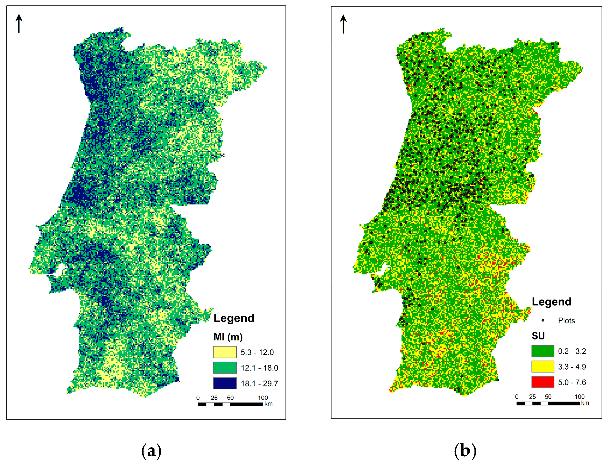
3.2. Species’ Productivity Modelling—A Sequential Gaussian Simulation Approach

The previous structural evaluation—variography—revealed no evidence of spatial anisotropy and, therefore, the omnidirectional variogram was used for the subsequent stochastic simulation technique (Figure 5).
The species’ spatial productivity map produced by the SGS approach highlights the highest productivities of timber (for fully-mature 35 year old trees) in the coastal center regions followed by the northern and central montane and submontane regions (Figure 6).

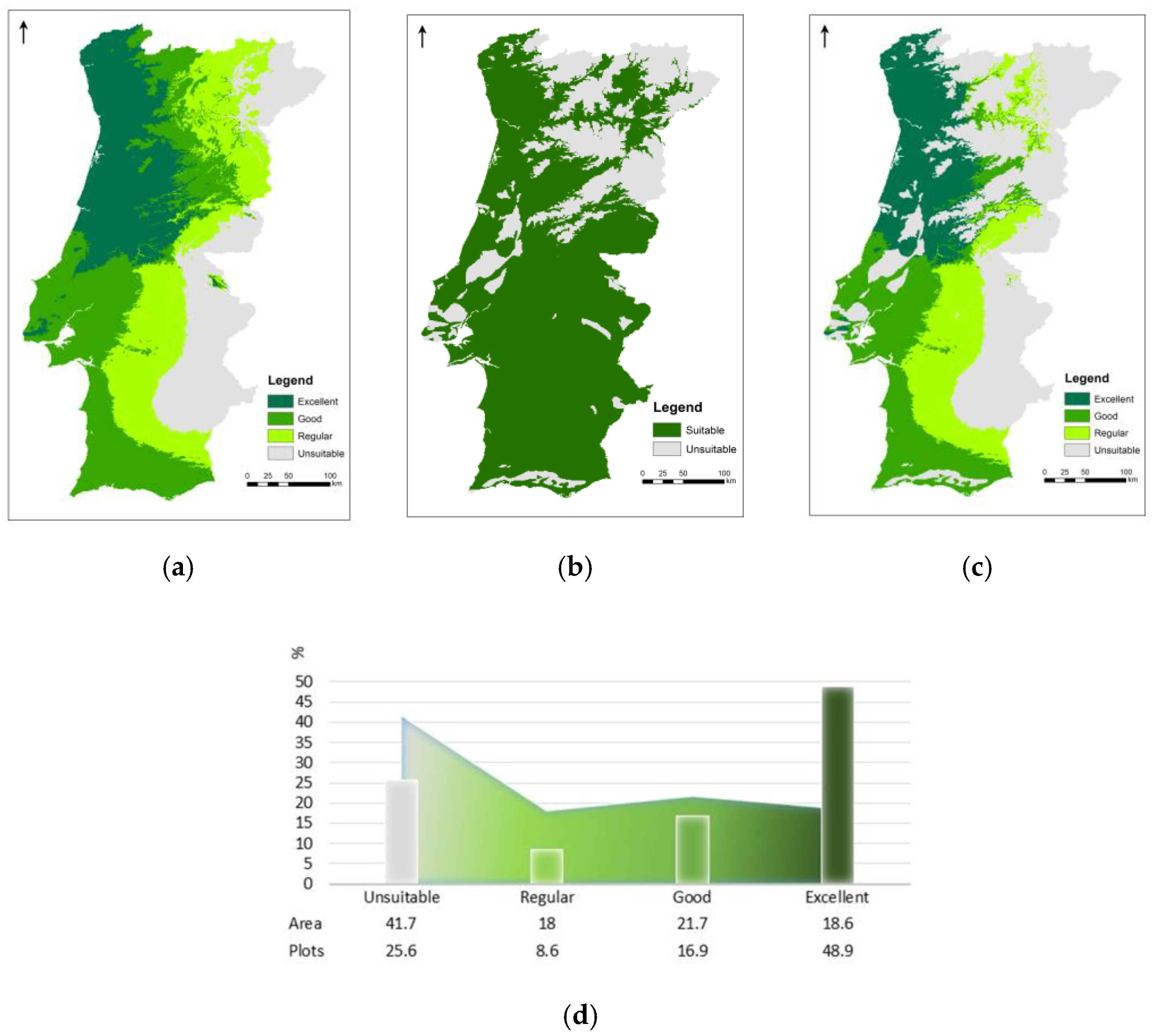
3.3. Species’ Ecological Envelope—Potential Distribution

The summary data for the species’ presence (Pb95 > 0) provides a few highlights about the ecological envelope variables range (Table 4) and the new computed thresholds through the ML classification tree algorithm, J48 (Table 5). A comparative assessment of these values allows one to conclude that the new defined thresholds are inside the range of the species’ presence and, therefore, consistent with the literature values (Table 5; Figure 7a,b). As expected, a broader range is observed when considering the species’ presence (Table 4) than when considering the species’ ecological envelope range, which sets the species’ potential distribution area (Figure 7c). As a result, the species’ potential distribution area was assessed in 60% of the country’s area and 78% of the species’ forest inventory plots (1995), as a dominant species, were found inside this ecological envelope (Figure 7c,d).

3.4. Species’ Afforestation and Management

The National Forest Inventory statistics (1965–2015) show the noticeable decrease in Maritime pine areas over the last 50 years (Figure 8a). Besides, as the species’ area decreased, a long-term damaging effect is observed in the stand age structure distribution of the past 20 years (1995–2005–2015) (Figure 8b–d). In 1995 (Figure 8b), Maritime pine forest had a regular age structure distribution. But in 2005 (Figure 8c), an important decrease in mature and old stands (>40 years) is already observed. The large wildfire which occurred in 2003 had a significant impact on the new stands’ increase by natural regeneration (<10 years). This trend was worse in 2015 (Figure 8d), with a massive increase in stands established by natural regeneration (<10 years) in opposition to the mature and old stands’ disappearance (>40 years). Again, 14 years after the 2003 wildfire, another large and extremely severe wildfire occurred in 2017. As a result, the young stands’ burnt area (<10 years; without viable seed production) will hardly recover by natural regeneration, so conversion to scrubland or other species is expected. From 1995 to 2015, the increase of uneven-aged stands was also observed, due to the absence of management (human desertification, forest owners ageing and lack of forest investment due to the high fire hazard) (Figure 8b,d).

4. Discussion

The results obtained in this study revealed that: (1) Maritime pine spatial distribution (Pb95 and P) modelling by ML approach provided a 69% and 65% fitting efficiency, respectively, while only a 43% fitting efficiency was obtained with the species’ productivity (SI35) modelling; (2) the species’ spatial productivity map corresponding to the SGS mean image (MI) shows the spatial distribution for high and low Maritime pine productivity spots in concordance with the results obtained when using the ML approach. Together, the approaches of the evaluation stresses two important points: (i) the species’ productivity is optimized in the northern coast (Atlantic influence) followed by the northern and central montane and submontane regions, and (ii) the obtained results overlap, given the two used techniques, validating the distribution of the associated spatial uncertainty and signaling a less robust assessment of the Maritime pine’s productivity in the south of the country; (3) the new obtained thresholds, through ML, were consistent with the literature [17,52], and refined the species’ potential distribution map. The species’ potential area was assessed in 60% of country’s area with 78% of the species’ forest inventory plots (1995) found inside this ecological envelope; and (4) the change in the Maritime pine stands’ age structure observed in the last decades put the species’ recovery by natural regeneration at risk.
The species spatial productivity map produced by the SGS approach uses the site index SI35 as a forest productivity indicator. This site index is highly linearly correlated to the site index SI50 (fitting efficiency of 90%) used in the PBRAVO growth and yield model for the species in Portugal. So, correspondence between the site index SI35 classes and timber productivities (e.g., mean annual increment at the age of 45 years) is possible. Low productivities (SI35 < 15 m) correspond to around 5 m3 ha year−1 or lower and high productivities (SI35 > 18 m) correspond to around 8 m3 ha year−1 or higher, which is in accordance with other studies and authors [56,57,58].
The species’ potential distribution map (ecological envelope) identifies the coastal strip in the north and center penetrating inland up to elevations of 700–900 m (e.g., smSA) as the Maritime pine distribution in Portugal. However, elevations from 0–400 m correspond to the most favorable sites (e.g., bSA, bMA, bAM, bsM). Current knowledge calls attention to the fact that the species does not well tolerate intense and prolonged colds and snow [17,52]. The species has severe limitations to growth in elevations above 800 m due to wind and snow, showing increased susceptibility to pests and diseases [17,52]. It was found that the species occurs in a variety of soil types, but mostly in cambisols molic, podzols haplic and regosols dystric [39]. Indeed, the species grows well in poor soil with light textures, preferably siliceous (e.g., podzols) [17,39].
Comparing the current Maritime pine distribution with the species’ potential distribution map, only 39% of species’ area stands in unsuitable sites compared to 51% in excellent and good sites. Regarding the productivity map, most of the species’ current distribution is in intermediate productive sites (56%), with high productive sites representing only 17%. When comparing the potential and productivity maps, a narrow concordance of only 28% between potential and productivity classes was obtained. Since forest productivity depends both on the environmental factors inherent to the site (climate, topography, and soil) and on management-related factors, it is possible that non-concordant classes (potentiality vs. productivity) can be explained to some extent by site micro-environmental conditions and/or species’ management (active/absent). Furthermore, the species’ range expansion in Portugal during the twentieth century (mainly due to human activity), and the extensive gene flow among populations related to this expansion, indicates that there is no genetic structure for the Portuguese populations of this species, meaning that the species is genetically homogeneous in the country [59].
Species management can be supported by applying the intensive management stand prescription, round wood production-oriented, as defended by Louro et al. [60], that uses artificial regeneration by plantation. In intense natural regeneration areas, a fully stocked stand prescription, pulp wood production-oriented, argued by Oliveira [17], is well suited. Moreover, the later prescription saves site preparation and plantation costs, being the most appropriate for the existing naturally regenerated Maritime pine stands of Portuguese private forest areas. It should be stressed that the two above recommendations were considered the most economically efficient in a study conducted for the Portuguese central inland species [58].
Forest planning and management at the local level is argued to be mandatory [26]. Firstly, the Forest Management Unit (FMU) must be organized into administrative units (units). Secondly, the Maritime pine forest must be identified by using the latest official land cover map and updated with the latest annual burnt area maps. Thirdly, the method for area control can be applied, following the species’ productivity map in defining the management compartments’ number and size, necessary to wood production regulation (annual constant production). The number of compartments is defined by the harvesting age, and the size of each compartment considering the site class productivity aiming to ensure a constant wood production in each year. Fourth, the silvicultural schedule is applied to each compartment, supported by the species’ potential distribution map, and will allow after harvesting the decision of whether to regenerate or to convert to another species or land use [9,26]. If the decision is to regenerate the Maritime pine stand, then measures to ensure natural regeneration sustainability should be considered.
In sum, the maps for the species’ current and potential distribution and productivity produced in this study allows us to identify the best sites for Maritime pine establishment, support this species’ wood production regulation and landscape planning, to decide about species’ diversity introduction (other products and services), and for fire hazard mitigation (fragmentation/compartmentalization). Furthermore, these maps were produced for the Maritime pine considering the entire country and with a higher resolution than others previously produced [7,13,61], as more detailed input data was used. Besides, the use of a ML approach to model species’ distribution model (SDM) and species’ productivity model (SPM) allowed us to validate the regressors’ variables used as covariates and to assess the resulting maps accuracy and precision, nonexistent information in previous studies. Moreover, it is worth noting that the seven-best selected regressor variables, either for the SDM and SPM, obtained in this study were consistent with the findings of a previous study [11]. Indeed, emphasizing that precipitation-related variables are more important in explaining the species’ distribution while a combination of temperature- and precipitation-related variables are important to explain species’ presence. On the other hand, elevation- and temperature-related variables are more important to explain the species’ productivity.
Additionally, in a similar study for Maritime pine in Spain, the best models selected for the species´ current distribution and productivity were the ML classification tree algorithm random forest and the ML regression tree algorithm by random forest, respectively [1]. These authors obtained an overall accuracy of 73% for the SDM and 60% for SPM, which is slightly higher than in the present study. This may be explained as in that study, more detailed data regarding the lithostratigraphy, geology and soil physical properties were used (e.g., bulk density of fine earth fraction (<2 mm); percentage of silt in soil; probability of occurrence of R horizon within 200 cm; depth to bedrock (R horizon) up to 200 cm; cation exchange capacity) [1].
Finally, further investigation is already being undertaken to compare maps’ agreement, for the present and for future projections under climate change scenarios, using the species’ distribution model (SDM) and species’ productivity model (SPM) fitted in this study and using the ML maximum entropy modelling by the MaxENT software.

5. Conclusions

Modelling species’ distribution and productivity are key to supporting integrated landscape planning, species afforestation, and sustainable forest management. Maritime pine forest area has decreased remarkably in the past years and requires urgent measures optimize recovery. The potential distribution map (ecological envelope) and the productivity map, obtained through a coupled stochastic-deterministic approach, are key for decision making on identifying the best sites for species afforestation, to apply the best management practices, and to improve species productivity. Post-fire areas in the best sites for the species should also be evaluated regarding the species’ natural regeneration capacity.
Since the species’ current and potential distributions and associated productivity were modeled using environmental covariates, such as climate attributes, their projection in future climate change scenarios is an achievable goal. This prospective view supports the design of future integrated planning, regarding fire hazard mitigation, and promoting forests multifunctionality and ecosystems services, under climate change scenarios.

Author Contributions

Conceptualization, C.A.; data curation, C.A., N.R. and T.A.; methodology, C.A., N.R. and T.A.; formal analysis, writing—original draft preparation, C.A. and T.A.; writing—review and editing, C.A., T.A., P.F. and M.M.R. All authors have read and agreed to the published version of the manuscript.

Funding

This study was funded by CERNAS-IPCB [UIDB/00681/2020 funding by Foundation for Science and Technology (FCT)]; CEF [UIDB/00239/2020 funding by FCT]; and under the Project UIDB/05183/2020 funding by FCT.

Institutional Review Board Statement

Not applicable.

Informed Consent Statement

Not applicable.

Data Availability Statement

All the data used in this study will be available upon request to the corresponding author.

Conflicts of Interest

The authors declare no conflict of interest.

Appendix A

Table A1. Soil codes and legend from the international soil classification system.
Code WRFBUGroupQualifier
2Water--
27FLeuFluvisolEutric
29CMdyCambisolDystric
30PZhaPodzolHaplic
35CMeuCambisolEutric
54SCglSolonchakGleyic
59ARhaArenosolHaplic
65VRpeVertisolPellic
67FLcaFluvisolCalcaric
72LPhaLeptosolHaplic
74RGdyRegosolDystric
76Urban--
87CMcaCambisolCalcaric
89LVglLuvisolGleyic
90LVccLuvisolCalcic
91PLeuPlanosolEutric
92LVhaLuvisolHaplic
107LVcrLuvisolChromic
108CMcrCambisolChromic
109RGeuRegosolEutric
119CMmoCambisolMollic
124UMarUmbrisolArenic
125VRcrVertisolChromic
127LVfrLuvisolFerric
129LVvrLuvisolFluvic
130ACglAcrisolGleyic
Table A2. Relative importance analysis to obtain a ranking regarding the significance of each regressor variable to the species distribution (Pb95 and P) and productivity (SI35) modelling in ML tree classification and regression.
TypeVariable RIPearsonRIPearsonRIPearson
P (n = 88,455) Pb95 (n = 88,455) SI50 (n = 739)
TemperatureT max31.33−0.0777824.030.079529.270.102
T min0.00−0.0033917.530.060953.240.1685
BIO116.62−0.042850.000.010744.160.1433
BIO259.66−0.1450390.780.270642.43−0.1385
BIO33.190.0109752.920.162298.740.2947
BIO446.38−0.1135198.570.2929100.00−0.2982
BIO555.73−0.1357187.320.260756.02−0.1762
T max Aug22.690.0572656.550.172657.820.1812
BIO61.880.0078528.990.093764.280.1991
T min Jan55.53−0.1352387.530.26135.98−0.0374
BIO750.27−0.12274100.000.29786.37−0.2604
BIO812.37−0.0327515.400.054874.410.2272
BIO943.92−0.1076861.470.186730.43−0.1052
BIO1046.69−0.1142461.440.186625.70−0.0921
BIO110.01−0.0034124.140.079872.170.221
PrecipitationBIO1296.230.2318896.330.286524.330.0883
BIO13100.000.2408296.540.287115.030.0625
BIO1452.240.1274254.420.16658.980.0457
BIO1538.77−0.0954533.920.107810.38−0.0496
BIO1698.450.2371599.550.295725.230.0908
BIO1773.210.1772270.630.212910.670.0504
BIO1873.660.1782981.870.245136.550.1222
BIO1999.380.2393598.080.291521.380.0801
TopographyE0.51−0.0046141.670.1389.44−0.2689
S37.450.092326.020.085242.00−0.1373
A11.220.0300211.420.04340.000.0208
SoilWRBFU26.650.0666629.270.094521.020.0791

References

  1. Barrio-Anta, M.; Castedo-Dorado, F.; Cámara-Obregón, A.; López-Sánchez, C. Predicting current and future suitable habitat and productivity for Atlantic populations of maritime pine (Pinus pinaster Aiton) in Spain. Ann. For. Sci. 2020, 77, 41. [Google Scholar] [CrossRef]
  2. Bede-Fazekas, A.; Levente Horváth, K.M. Impact of climate change on the potential distribution of Mediterranean pines. Q. J. Hung. Meteorol. Serv. 2014, 118, 41–52. [Google Scholar]
  3. Deus, E.; Silva, J.S.; Castro-Díez, P.; Lomba, A.; Ortiz, M.L.; Vicente, J. Current and future conflicts between eucalypt plantations and high biodiversity areas in the Iberian Peninsula. J. Nat. Conserv. 2018, 45, 107–117. [Google Scholar] [CrossRef]
  4. Ribeiro, M.M.; Roque, N.; Ribeiro, S.; Gavinhos, C.; Castanheira, I.; Quinta-Nova, L.; Albuquerque, T.; Gerassis, S. Bioclimatic modeling in the Last Glacial Maximum, Mid-Holocene and facing future climatic changes in the strawberry tree (Arbutus unedo L.). PLoS ONE 2019, 14, e0210062. [Google Scholar] [CrossRef] [Green Version]
  5. Hock, B.K.; Payn, T.W.; Shirley, J.W. Using a geographical information system and geostatistics to estimate site index of Pinus radiata for Kaingaroa Forest. N. Z. J. For. Sci. 1993, 23, 264–277. [Google Scholar]
  6. Payn, T.W.; Hill, R.B.; Hock, B.K.; Skinner, M.F.; Thorn, A.J.; Rijkse, W.C. Potential for the use of GIS and spatial analysis techniques as tools for monitoring changes in forest productivity and nutrition, a New Zealand example. For. Ecol. Manag. 1999, 122, 187–196. [Google Scholar] [CrossRef]
  7. Santos, C.; Almeida, J. Caracterização espacial de um índice de produtividade nos povoamentos de pinheiro bravo em Portugal. Finisterra Rev. Port. De Geogr. 2003, 75, 51–65. (In Portuguese) [Google Scholar] [CrossRef] [Green Version]
  8. Pelissari, A.L.; Caldeira, S.F.; Filho, F.A.; Amaral, M.S. Propostas de mapeamentos da capacidade produtiva de sítios florestais por meio de análises geoestatísticas. Sci. For. 2015, 43, 601–608. [Google Scholar]
  9. Mestre, S.; Alegria, C.; Teresa, M.; Albuquerque, D.; Goovaerts, P. Developing an index for forest productivity mapping—A case study for maritime pine production regulation in Portugal. Rev. Árvore 2017, 41, e410306. [Google Scholar] [CrossRef]
  10. Parresol, B.R.; Scott, D.A.; Zarnoch, S.J.; Edwards, L.A.; Blake, J.I. Modeling forest site productivity using mapped geospatial attributes within a South Carolina Landscape, USA. For. Ecol. Manag. 2017, 406, 196–207. [Google Scholar] [CrossRef]
  11. Alegria, C.; Roque, N.; Albuquerque, T.; Gerassis, S.; Fernandez, P.; Ribeiro, M.M. Species ecological envelopes under climate change scenarios: A case study for the main two wood-production forest species in Portugal. Forests 2020, 11, 880. [Google Scholar] [CrossRef]
  12. Fourcade, Y.; Engler, J.O.; Rodder, D.; Secondi, J. Mapping species distributions with MAXENT using a geographically biased sample of presence data: A performance assessment of methods for correcting sampling bias. PLoS ONE 2019, 9, e97122. [Google Scholar] [CrossRef] [Green Version]
  13. ICNF. Planos Regionais de Ordenamento Florestal; Instituto da Conservação da Natureza e das Florestas, Lisboa. 2019. Available online: http://www2.icnf.pt/portal/florestas/profs/prof-em-vigor (accessed on 20 February 2020). (In Portuguese).
  14. DGRF. Plano Regional de Ordenamento Florestal do Pinhal Interior Sul; Documento estratégico; Direção Geral dos Recursos Florestais: Lisbon, Portugal, 2005. (In Portuguese) [Google Scholar]
  15. ICNF. FN6—Áreas dos Usos do Solo e das Espécies Florestais de Portugal Continental. Resultados Preliminares; Instituto da Conservação da Natureza e das Florestas, Lisboa. 2013. Available online: http://www2.icnf.pt/portal/florestas/ifn/resource/doc/ifn/ifn6-res-prelimv1-1 (accessed on 20 February 2020). (In Portuguese).
  16. ICNF. 6° Inventário Florestal Nacional—IFN6. 2015. Relatório Final; Instituto da Conservação da Natureza e das Florestas, Lisboa. 2019. Available online: http://www2.icnf.pt/portal/florestas/ifn/resource/doc/ifn/ifn6/IFN6_Relatorio_completo-2019-11-28.pdf (accessed on 20 February 2020). (In Portuguese).
  17. Oliveira, A. Boas Práticas Florestais para o Pinheiro Bravo. Manual; Centro Pinus, Porto. 1999. Available online: https://centropinus.org/files/2018/04/manual01.pdf (accessed on 12 November 2020). (In Portuguese).
  18. DR. Estratégia Nacional para as Florestas, Resolução de Conselho de Ministros n° 6-B/2015, Diário da República, I Série—n° 24 de 4 de fevereiro. 2015. Available online: https://dre.pt/application/file/66432612 (accessed on 9 March 2018). (In Portuguese).
  19. ICNF. Estatísticas. Incêndios Florestais—Totais Anuais (Nacionais, Por Distrito e por Freguesia). Área Ardida Por Tipo de Ocupação de Solos. Lisboa, Instituto da Conservação da Natureza e Florestas. 2017. Available online: http://www.icnf.pt/portal/florestas/dfci/inc/estat-sgif (accessed on 9 March 2018). (In Portuguese).
  20. Soares, P.; Calado, N.; Carneiro, S. Manual de Boas Práticas Para o Pinheiro-Bravo. Centro Pinus, Porto. 2020. Available online: https://centropinus.org/files/2020/05/Silvicultura_Centro-Pinus_digital.pdf (accessed on 12 November 2020).
  21. Calvo, L.; Hernández, V.; Valbuena, L.; Taboada, A. Provenance and seed mass determine seed tolerance to high temperatures associated to forest fires in Pinus pinaster. Ann. For. Sci. 2016, 73, 381–391. [Google Scholar] [CrossRef] [Green Version]
  22. Alegria, C.; Teixeira, M.C. An overview of maritime pine private non-industrial forest in the centre of Portugal: A 19-year case study. Folia For. Pol. 2016, 58, 198–213. [Google Scholar] [CrossRef] [Green Version]
  23. Nurek, T.; Gendek, A.; Roman, K.; Dąbrowska, M. The Impact of Fractional Composition on the Mechanical Properties of Agglomerated Logging Residues. Sustainability 2020, 12, 6120. [Google Scholar] [CrossRef]
  24. Nurek, T.; Gendek, A.; Roman, K. Forest Residues as a Renewable Source of Energy: Elemental Composition and Physical Properties. BioResources 2018, 14, 6–20. Available online: https://ojs.cnr.ncsu.edu/index.php/BioRes/article/view/BioRes_14_1_6_Nurek_Forest_Residues_Renewable_Energy/6480 (accessed on 23 February 2021). [CrossRef]
  25. Nurek, T.; Gendek, A.; Roman, K.; Dąbrowska, M. The effect of temperature and moisture on the chosen parameters of briquettes made of shredded logging residues. Biomass Bioenergy 2019, 130, 105368. [Google Scholar] [CrossRef]
  26. Navalho, I.; Alegria, C.; Quinta-Nova, L.; Fernandez, P. Integrated planning for landscape diversity enhancement, fire hazard mitigation and forest production regulation: A case study in central Portugal. Land Use Policy 2017, 61, 398–412. [Google Scholar] [CrossRef]
  27. Fernandes, P.M. Combining forest structure data and fuel modelling to classify fire hazard in Portugal. Ann. For. Sci. 2009, 66, 415. [Google Scholar] [CrossRef] [Green Version]
  28. Fernandes, P.M.; Luz, A.; Loureiro, C. Changes in wildfire severity from maritime pine woodland to contiguous forest types in the mountains of northwestern Portugal. For. Ecol. Manag. 2010, 260, 883–892. [Google Scholar] [CrossRef]
  29. Fernandes, P.M.; Loureiro, C.; Guiomar, N.; Pezzatti, G.B.; Manso, F.T.; Lopes, L. The dynamics and drivers of fuel and fire in the Portuguese public forest. J. Environ. Manag. 2014, 146, 373–382. [Google Scholar] [CrossRef]
  30. Davis, L.; Johnson, K. Forest Management, 3rd ed.; McGraw-Hill Education: New York, NY, USA, 1987. [Google Scholar]
  31. DGT. Catálogo de Serviços de Dados Geográficos; Direção Geral do Território, Lisboa. 2020. Available online: https://snig.dgterritorio.gov.pt/rndg/srv/por/catalog.search#/search?anysnig=COS&fast=index (accessed on 20 February 2020).
  32. IPMA. Clima de Portugal Continental. Instituto Português do Mar e da Atmosfera. 2021. Available online: https://www.ipma.pt/pt/educativa/tempo.clima/ (accessed on 1 March 2021).
  33. DGT. Especificações Técnicas da Carta de Uso e Ocupação do Solo de Portugal Continental para 1995, 2007, 2010 e 2015. Relatório Técnico; Direção-Geral do Território, Lisboa. 2018. Available online: http://www.dgterritorio.pt/cartografia_e_geodesia/cartografia/cartografia_tematica/cartografia_de_uso_e_ocupacao_do_solo__cos_clc_e_copernicus_/ (accessed on 27 July 2019).
  34. ICNF. Inventário Florestal Nacional. IFN4. Dados de Base de 1995-98. ICNF: Lisboa, Portugal. 2020. Available online: http://www2.icnf.pt/portal/florestas/ifn/ifn4/dad-base95-98 (accessed on 11 August 2020). (In Portuguese).
  35. Hijmans, R.J.; Cameron, S.E.; Parra, J.L.; Jones, P.G.; Jarvis, A. Very high-resolution interpolated climate surfaces for global land areas. Int. J. Climatol. 2005, 25, 1965–1978. [Google Scholar] [CrossRef]
  36. NASA JPL. NASA Shuttle Radar Topography Mission Global 1 arc second [Data Set]. NASA EOSDIS Land Processes DAAC. 2013. Available online: http://doi.org/10.5067/MEaSUREs/SRTM/SRTMGL1.003 (accessed on 9 March 2018).
  37. Panagos, P. The European soil database. GEO Connex. 2006, 5, 32–33. [Google Scholar]
  38. Van Liedekerke, M.; Jones, A.; Panagos, P. ESDBv2 Raster Library—A Set of Rasters Derived from the European Soil Database Distribution v2.0 (CD-ROM, EUR 19945 EN); European Commission and the European Soil Bureau Network. 2006. Available online: https://esdac.jrc.ec.europa.eu/content/european-soil-database-v2-raster-library-1kmx1km (accessed on 29 July 2018).
  39. IUSS Working Group WRB. World Reference Base for Soil Resources 2014, Update 2015 International Soil Classification System for Naming Soils and Creating Legends for Soil Maps; World Soil Resources Reports No. 106; FAO: Rome, Italy, 2015. [Google Scholar]
  40. Vanclay, J. Modeling Forest Growth and Yield. Applications to Mixed Tropical Forests; CAB International: Wallingford, UK, 1994. [Google Scholar]
  41. Páscoa, F.; Bento, J.; Marques, C. Previsão da Produção Lenhosa Para o Período 1988/2048; ACEL: Lisboa, Portugal, 1989. Inventário Florestal, Pinheiro Bravo. (In Portuguese) [Google Scholar]
  42. WEKA. WEKA Software. Machine Learning Group at the University of Waikato: Waikato, New Zealand. 2020. Available online: https://www.cs.waikato.ac.nz/ml/weka/ (accessed on 11 August 2020).
  43. Hall, M.; Frank, E.; Holmes, G.; Pfahringer, B.; Reutemann, P.; Witten, I.H. The WEKA data mining software: An update. SIGKDD Explor. 2009, 11, 10–18. [Google Scholar] [CrossRef]
  44. Breiman, L. Random forests. Mach. Learn. 2001, 45, 5–32. [Google Scholar] [CrossRef] [Green Version]
  45. Witten, I.H.; Frank, E.; Hall, M.A. Data Mining: Practical Machine Learning Tools and Techniques; Morgan Kaufmann: Burlington, VT, USA, 2011. [Google Scholar]
  46. Ryan, T.P. Modern Regression Methods; John Wiley & Sons: New York, NY, USA, 1997. [Google Scholar]
  47. Nussbaumer, R.; Mariethoz, G.; Gloaguen, E.; Holliger, K. Which path to choose in sequential Gaussian simulation. Math. Geosci. 2018, 50, 97–120. [Google Scholar] [CrossRef]
  48. Albuquerque, M.; Gerassis, S.; Sierra, C.; Taboada, J.; Martín, J.; Antunes, I.; Gallego, J. Developing a new Bayesian risk index for risk evaluation of soil contamination. Sci. Total Environ. 2017, 603–604, 167–177. [Google Scholar] [CrossRef]
  49. Goovaerts, P. Geostatistics for Natural Resources Evaluation. Applied Geostatistics; Oxford University Press: New York, NY, USA, 1997; p. 496. [Google Scholar]
  50. Soares, A.; Nunes, R.; Azevedo, L. Integration of uncertain data in geostatistical modelling. Math. Geosci. 2017, 49, 253–273. [Google Scholar] [CrossRef]
  51. Alves, A.A.M. Técnicas de Produção Florestal; Instituto Nacional de Investigação Científica: Lisbon, Portugal, 1988. (In Portuguese) [Google Scholar]
  52. Alves, A.M.; Pereira, J.S.; Correia, V.A. Silvicultura. A Gestão dos Ecossistemas Florestais; Fundação Calouste Gulbenkian: Lisbon, Portugal, 2012. (In Portuguese) [Google Scholar]
  53. AFN. Inventário Florestal Nacional Portugal Continental. 5º Inventário Florestal Nacional 2005–2006. Apresentação do Relatório Final. Available online: http://www2.icnf.pt/portal/florestas/ifn/resource/doc/ifn/Apresenta-IFN5-AFN-DNGF-JP.pdf (accessed on 11 August 2020). (In Portuguese).
  54. DGR. Inventário Florestal Nacional Portugal Continental. 3ª Revisão, 1995–1998. Relatório Final; Direçção-Geral das Florestas (DGR): Lisboa, Portugal, 2010. (In Portuguese) [Google Scholar]
  55. AFN. Inventário Florestal Nacional Portugal Continental. 5º Inventário Florestal Nacional 2005–2006. FloreStat—Aplicação para a Consulta dos Resultados do 5° Inventário Florestal Nacional. Autoridade Florestal Nacional (AFN): Lisboa, Portugal. 2010. Available online: http://www.icnf.pt/portal/florestas/ifn/ifn5/relatorio-final-ifn5-florestat-1 (accessed on 11 August 2020). (In Portuguese).
  56. Santos, C.; Almeida, J.A. Spatial characterization of maritime pine productivity in Portugal. In Forest Context and Policies in Portugal. World Forests; Reboredo, F., Ed.; Springer: Cham, Switzerland, 2014; Volume 19, pp. 185–217. [Google Scholar] [CrossRef]
  57. Oliveira, A.C.; Pereira, J.S.; Correia, A.V. A Silvicultura do Pinheiro Bravo. Manual; Centro Pinus: Porto, Portugal, 2000. [Google Scholar]
  58. Alegria, C. Simulation of silvicultural scenarios and economic efficiency for maritime pine (Pinus pinaster Aiton) wood-oriented management in centre inland of Portugal. Investig. Agrar. Sist. Recur. For. Syst. 2011, 20. [Google Scholar] [CrossRef] [Green Version]
  59. Ribeiro, M.M.; Plomion, C.; Petit, R.; Vendramin, G.G.; Szmidt, A.E. Variation in chloroplast single-sequence repeats In Portuguese maritime pine (Pinus pinaster Ait.). Theor. Appl. Genet 2001, 102, 97–103. [Google Scholar] [CrossRef]
  60. Louro, G.; Marques, H.; Salinas, F. Elementos de Apoio à Elaboração de Projectos Florestais, 2nd ed.; Estudos e Informação n° 321, Direcção Geral das Florestas—DGF, Lisboa. 2002. Available online: http://www2.icnf.pt/portal/florestas/gf/documentos-tecnicos/resource/doc/Elaboracao-projetos-florestais_2ed-EI-321_Louro-Marques-Salinas_DGF_2002b.pdf (accessed on 11 August 2020). (In Portuguese).
  61. Pereira, J.S.; Correia, A.V.; Correia, C.V.; Ferreira, M.T.; Onofre, N.; Freitas, H.; Godinho, F. Florestas e biodiversidade. In Alterações Climáticas em Portugal. Cenários, Impactos e Medidas de Adaptação (Projecto SIAM II); Santos, F.D., Miranda, P.M.A., Eds.; Gradiva: Lisbon, Portugal, 2006; pp. 301–344. [Google Scholar]
Figure 1. Maritime pine study area: (a) land cover map (COS 1995); and (b) forest inventory plots (1995) in pure Maritime pine stands (n = 739).
Forests 12 00368 g001
Figure 2. Maritime pine empirical distribution: (a) forest regions in Portugal [52]; and (b) Maritime pine occupation by Oliveira [17]. Forest regions of Maritime pine occurrence (in bold). bSA—basal Sub-Atlantic; bMA—basal Mediterranean–Atlantic; bAM—basal Atlantic–Mediterranean; bsM—basal sub-Mediterranean; and smSA—sub-montane sub-Atlantic.
Forests 12 00368 g002
Figure 3. ML models maps and residuals: (a) species distribution maps (Pb95) and residual for ME and MR models simulations; and (b) species productivity maps (SI35) and residual for ME and MR model simulations.
Forests 12 00368 g003
Figure 4. Soil data (n = 88,455)—occurrence and distribution of the WRFBU codes.
Forests 12 00368 g004
Figure 5. (a) Directional variograms (angle lag 30°; tolerance 15°); and (b) adopted omnidirectional variogram.
Forests 12 00368 g005
Figure 6. Maritime pine forest productivities by back-transformed sequential Gaussian simulation. (a) Site index map —SI35 mean image (MI), and (b) back-transformed standard deviation (SU). Legend: SI30—stand dominant height (m) at the age of 35 years; MI—mean image of 100 computed scenarios through back-transformed SGS (sequential Gaussian simulation); SU—spatial uncertainty (back-transformed standard deviation).
Forests 12 00368 g006
Figure 7. Maritime pine potential distribution (i.e., ecological envelope) map algebra. (a) Temperature annual range, temperature limits and precipitation ranking (BIO7 + (BIO6 × BIO5) + BIO12). (b) Elevation and soil constrains (E × WRFBU). (c) Potential distribution map ((BIO7 + (BIO6 × BIO5) + BIO12) × E × WRFBU); and (d) area (ha) and plots distribution (%) by suitability class. Legend: Excellent (sum equal 3—without temperature range, temperature limits and precipitation limitations); 2—Good (sum equals 2—with one limitation); 1—Regular (sum equals 1—with two limitation); 0—Unsuitable (null); Boolean maps (0—Not suitable, 1—Suitable).
Forests 12 00368 g007
Figure 8. Maritime pine forest National Forest Inventory statistics. (a) Area (1965–2015); (b) area by stand age classes (1995); (c) area by stand age classes (2005); and (d) area by stand age classes (2015).
Forests 12 00368 g008
Table 1. Climatic, topographic, and soil variables.
TypeVariableUnitsDescription
TemperatureT max°C 10−1Monthly average maximum temperature
T min°C 10−1Monthly average minimum temperature
BIO1°C 10−1Annual mean temperature
BIO2°C 10−1Mean diurnal range (mean of monthly (max temp–min temp))
BIO3%Isothermality B I O 3 = 100 . B I O 2 . B I O 7 1    
BIO4%Temperature seasonality (standard deviation ×100)
BIO5°C 10−1Maximum temperature of the warmest month
T max Aug°C 10−1Maximum temperature in August
BIO6°C 10−1Minimum temperature of the coldest month (i.e., winter frost)
T min Jan°C 10−1Minimum temperature in January
BIO7°C 10−1Temperature annual range B I O 7 = B I O 5 B I O 6    
BIO8°C 10−1Mean temperature of the wettest quarter
BIO9°C 10−1Mean temperature of the driest quarter
BIO10°C 10−1Mean temperature of the warmest quarter
BIO11°C 10−1Mean temperature of the coldest quarter
PrecipitationBIO12mmAnnual precipitation
BIO13mmPrecipitation of the wettest month
BIO14mmPrecipitation of the driest month
BIO15%Precipitation seasonality (coefficient of variation)
BIO16mmPrecipitation of the wettest quarter
BIO17mmPrecipitation of the driest quarter
BIO18mmPrecipitation of the warmest quarter
BIO19mmPrecipitation of the coldest quarter
TopographyEmElevation—The vertical distance measured between a point and a datum (a reference surface) which is usually the mean sea level (MSL)
S%Slope—The rate of change of elevation for each digital elevation model (DEM) cell (i.e., the first derivative of a DEM)
A°Aspect—The orientation of slope measured clockwise in degrees from 0 to 360, where 0 is north-facing, 90 is east-facing, 180 is south-facing, and 270 is west-facing.
SoilWRBFU Soil codes from the international soil classification system for naming soils and creating legends for soil maps.
Table 2. Species distribution and productivity of ML models. Performance statistics (after the 10-fold cross-validation approach) for the best ML regression and classification trees algorithms essayed: M5P or J48, respectively; random forests (RF); and random tree (RT).
ML Tree Regression Models—Species Distribution Models (Pb95) (n = 88,455)
Regressor variablesM5P RFRT
R2R2R2
(MAE)(MAE)(MAE)
ME—BIO5, BIO6, BIO7, BIO12, E, WRBFU0.66880.69340.5356
(5.9535)(5.5021)(6.5937)
MR—BIO13, BIO19, BIO16, BIO12, BIO18, BIO17, BIO20.65320.65550.5322
(6.2138)(5.7823)(6.5820)
ML Tree Classification Models—Species distribution models (P) (n = 88,455)
Regressor variablesJ48 RF RT
KappaKappaKappa
(MAE)(MAE)(MAE)
ME—BIO5, BIO6, BIO7, BIO12, E, WRBFU0.64250.65240.5789
(0.1893)(0.1701)(0.1654)
MR—BIO7, BIO16, BIO4, BIO19, BIO13, BIO12, BIO20.6298 0.6427 0.5613
(0.1937)(0.1761)(0.1724)
ML Tree Regression Models—Productivity models (SI35) (n = 739)
Regressor variablesM5P RF RT
R2R2R2
(MAE)(MAE)(MAE)
ME—BIO5, BIO6, BIO7, BIO12, E, WRBFU0.3727 0.4261 0.2247
(2.9650)(2.9093)(3.9190)
MR—BIO4, BIO3, E, BIO7, BIO8, BIO11, BIO60.3845 0.4170 0.2634
(2.9473)(2.9339)(3.7945)
Legend: Models essayed: ME (conceptual environmental variables) and MR (variables selected by the search Rankers method). Model performance statistics: R2—pseudo-coefficient of determination; Kappa—Cohen’s kappa statistic; and MAE—mean absolute error (in brackets). Temperature-related variables BIO2—Mean diurnal range (°C); BIO3—Isothermality (%); BIO4—Temperature seasonality (%); BIO5—Maximum temperature of the warmest month (°C); BIO6—Minimum temperature of the coldest month (°C); BIO7—Temperature annual range (°C). Precipitation-related variables BIO12—Annual precipitation (mm); BIO13—Precipitation of the wettest month (mm); BIO14—Precipitation of the driest month (mm); BIO15—Precipitation seasonality (%); BIO16—Precipitation of the wettest quarter (mm); BIO17—Precipitation of the driest quarter (mm); BIO18—Precipitation of the warmest quarter (mm); BIO19—Precipitation of the coldest quarter (mm); Topographic related variables E—Elevation (m). Soil-related variables WRBFU—soil codes; Pb95—species grid percentage coverage (0–100); P—species presence (1)/absence (0); SI35—stand dominant height (m) at the age of 35 years using the model by Páscoa et al. [35].
Table 3. Selected ML models (ME) for species distribution and productivity. Regressor variables summary data.
Species Distribution (Pb95) (n = 88,455)Species Productivity (SI35) (n = 739)
Type Variables Min.Max.MeanSDMin.Max.MeanSD
TemperatureBIO519.734.028.62.522.131.927.32.1
BIO6−2.89.25.02.3−1.18.34.81.9
BIO712.229.323.62.914.127.922.52.9
PrecipitationBIO12463.01792.0840.7269.9483.01593.01015.6211.5
TopographyE0.01921.0321.1262.60.01275.0329.6248.5
Legend: Temperature-related variables BIO5—Maximum temperature of the warmest month (°C); BIO6—Minimum temperature of the coldest month (°C); BIO7—Temperature annual range (°C); Precipitation-related variables BIO12—Annual precipitation (mm); Topographic-related variables E—Elevation (m); and Soil-related variables Pb95—species grid percentage coverage (0–1); SI35—stand dominant height (m) at the age of 35 years using the model by Páscoa et al. [41]; Min.—minimum; Max.—maximum; SD—standard deviation.
Table 4. Summary data for species presence in COS 1995 (Pb95 > 0).
Maritime Pine—Pb95 > 0 (n = 23,752)
TypeVariableUnitsMin.Max.MeanStd. Dev.
TemperatureBIO5°C21.832.727.52.2
T max Aug°C21.832.727.52.2
BIO6°C−1.49.05.41.7
T min Jan°C−2.49.33.42.0
BIO7°C13.328.222.12.9
T max Aug–T min Jan°C14.131.024.13.2
PrecipitationBIO12mm468.01587.0968.3221.3
TopographyEm0.01192.0264.9200.7
Legend: Temperature-related variables BIO5—Maximum temperature of the warmest month (°C); BIO6—Minimum temperature of the coldest month (°C); BIO7—Temperature annual range (°C); Precipitation-related variables BIO12—Annual precipitation (mm); and Topographic-related variables E—Elevation (m).
Table 5. Maritime pine potential distribution (i.e., ecological envelope)—new thresholds obtained by ML classification tree algorithm J48.
Temperature Range
(°C)
Temperature Limits
(°C)
Precipitation (mm)Elevation
(m)
WRFBU
BIO7 ≤ 25.1BIO6 > 2.6
BIO5 < 29.8
P > 821E < 731Soils different of LVcc, CMca, and FLca
Legend: Temperature-related variables BIO7—Temperature annual range (°C); BIO6—Minimum temperature of the coldest month (°C); BIO5—Maximum temperature of the warmest month (°C); Precipitation-related variables BIO12—Annual precipitation (mm); Topographic-related variables E—Elevation (m); and Soil related variables WRFBU—soils different of luvisols calcic (LVcc), cambisols calcarean (CMca), and fluvisols calcic (FLca).
Publisher’s Note: MDPI stays neutral with regard to jurisdictional claims in published maps and institutional affiliations.

