Spatial Distribution of Forest Ecosystem Service Benefits in Germany: A Multiple Benefit-Transfer Model

Abstract

We investigate the economic benefits of fundamental forest ecosystem services (FES) for the population in Germany at national level in monetary terms and estimate the spatial distribution of these benefits at county level. Specifically, we consider the benefits of timber production, of global climate protection due to carbon sequestration, of recreation for local residents, and of services for nature protection and landscape amenity. Combining information from official statistics and data from valuation studies that are compatible with economic demand theory, we identify spatial drivers of FES benefits and derive generic valuation functions for each of the services. Using a Geographic Information System, these valuation functions are applied to the conditions in the Local Administrative Units (municipalities), resulting in Benefit Function Transfer estimates for each service and each municipality. Afterwards, results are aggregated to NUTS-3 level (counties) and mapped. Aggregate annual benefits of timber production to society as a whole, of climate protection and of recreation services together exceed the ten billion Euro mark—far more than what is reflected in market statistics. Scenarios illustrate the potential for enhancing nature protection benefits particularly by restoring forest biodiversity, as measured by an avifaunistic indicator. The spatial analysis reveals distinct distributional patterns for each of the services. We conclude that a spatially explicit valuation for an entire country is possible even with limited data, which can help policy makers improve the institutional setting in a way that the protection and use of the forests become more sustainable and efficient. After pointing at several caveats, we finally suggest various possibilities for further model development.

1. Introduction

The Millennium Ecosystem Assessment of the United Nations (MEA) has highlighted how extensively human societies benefit from the services provided by biodiverse ecosystems in general and by forests in particular [1,2]. In the subsequent studies on the “Economics of Ecosystems and Biodiversity” (TEEB), the manifold interdependencies between economy and nature and their influence on human well-being were demonstrated from an international perspective [3,4,5] as well as for individual countries, including Germany [6,7,8,9]. Both MEA and TEEB take global threats to biodiversity and to the sustainable use of natural resources as their starting point. Economically, such threats can be traced back to distorted market signals: Many services provided by ecosystems are non-marketable and remain unpriced (i.e., they are “public goods”), causing markets to reflect neither their benefits nor the costs of their consumption. Market signals may therefore misguide decisions about resource utilization (i.e., the problem of externalities) [10,11].

Nevertheless, it is possible to quantify the values that people assign to unpriced ecosystem services, even in monetary terms. Such valuations help to make the value of unpriced services tangible in comparison to the value of marketable goods, to reveal trade-offs and to depict scarcities [12]. If undertaken from the consumer perspective, economic valuations inform about the benefits people derive from a service. Individual monetary benefits can then be interpreted as (cardinal) indicators of (ordinal) individual utility (for some associated problems, see [13,14]). The TEEB studies illustrate how benefits of virtually all ecosystem services can be valued in monetary units with methods grounded in economic welfare theory and provide a wealth of examples [5].

The central problem for a comprehensive economic valuation of ecosystem services is thus not the lack of suitable methods. Very often, however, there is a lack of empirical application at a policy-relevant level. Despite years of research (as documented, e.g., in several specialized databases [15,16,17]), the available information about (forest) ecosystem benefits remains fragmentary. Much of the literature focuses on site-specific, case-specific, or methodological particularities, and studies differ substantially with respect to their spatial scope, purpose, disciplinary basis, and the services evaluated [18]. In addition, the definitions of the latter are often not mutually comparable, impeding a systematic overview of the respective service spectrum and its comprehensive spatial analysis at larger scale. Against this background, the Biodiversity Strategy of the European Commission emphasizes the need for mapping and assessment of ecosystem services (MAES) and calls upon the member states to map the state of ecosystems and their services in their national territories [(by 2014)], to assess the economic value of such services, and to integrate the values into their reporting [(by 2020)] [19].

In response, the European Union has launched the MAES initiative [20,21], and several member countries have elaborated national TEEB studies and/or National Ecosystem Assessments (NEA), albeit in very different depth and detail [22]. However, even under this umbrella, comprehensive and spatially differentiated economic valuations of ecosystem services are rare. An early and very comprehensive example is the NEA of the United Kingdom, which has been issued already before the EU Biodiversity Strategy [23,24]; an update was published in 2014, part of which specifically addressed economic benefits of ecosystem services [25]. Drawing on extensive experience with the economic valuation of ecosystem services in the UK, the British NEA covers the major land use forms, including forestry, and presents spatially differentiated benefit estimates of various ecosystem services of forests and other land uses for the whole country (including timber production, water quality, greenhouse gas reduction, recreation, and biodiversity services), under the status quo as well as under different future scenarios [26]. The Spanish NEA [27,28] addresses economic benefits of a variety of ecosystem services, some of which are also spatially differentiated and mapped (i.e., agricultural production, recreational and water related services); forestry, however, plays but a marginal role here. Other national studies address various forest ecosystem services (FES) and their economic benefits, too, but limit the results either to a number of illustrative case studies or to average or aggregate values at national level, without systematically analyzing and mapping the spatial distribution of benefits for the respective country as a whole. Examples are the Norwegian NEA [29,30], Finland’s TEEB study [31], the NEA of France in its first phase [32], an Austrian study on FES benefits [33,34,35,36] commissioned by the Austrian Federal Forests (who manage about 22% of the Austrian territory), and finally, the German TEEB study [7,8]. Other NEAs do not address economic FES benefits at all [22], often so because they lack the necessary data basis.

In short: Even if some information about the economic benefits of FES is available in European countries, not much is known about their spatial distribution. However, particular FES benefits may vary strongly within a country [25]—and even more so across countries, as preferences of people differ due to cultural traditions and socioeconomic structures, as well as due to different characteristics of their forests and their silvicultural history [37,38,39].

The problem of spatially distributing data to smaller scale levels exists in many domains. The spatial distribution of national data across regions is often applied in economic studies, e.g., for calculating the specialization of certain sectors or economic activities in the regions of a country by location quotients when appropriate survey data are missing [40]. While various location quotients have been tested and parameterized for regional distributions of sectoral employment (as regionalized employment data are usually available), applications in conservation studies are very rare. Overall, the problem remains that regionalized data of indicator variables must be available for appropriate parametrization and model control, regardless of the methods applied.

Against this background, the present article aims to identify FES benefits and their spatial variability in Germany, in a way that also allows scenario analyses of alternative forest management approaches. This can help policy makers identify regional trade-offs between services and exploit potential for optimization, for example in the development of the legal and economic framework for forest management. Methodologically, our study applies a benefit function transfer approach: we analyze data from domestic valuation studies that are in line with demand theory, identify spatial value determinants, and translate them into a generic valuation function for each FES. This function is then applied to estimate the respective FES benefits in each German municipality.

Specifically, the article focuses on timber production, global climate protection due to carbon sequestration, recreation of local residents, and on services for nature protection and landscape amenity, thus covering provisioning, regulating as well as cultural ecosystem services according to the CICES typology [41,42]. The following section first gives a short overview and explains the GIS database that links the valuation functions to the local conditions in the municipalities. Afterwards it describes our quantification approach for each of these services as well as the valuation methods applied. The results section presents aggregated benefit estimates for the entire country, validates these by a comparison to reference values (if available), and subsequently shows the spatial distribution of the benefits. Finally, we discuss several caveats that should be considered when interpreting the results, indicate various possibilities for further development of our model, and draw conclusions for valuation practice and forest policy.

2. Materials and Methods

2.1. Basic Model Description and Geo-Database

The benefit transfer model is implemented under the geographical information system ESRI ArcGIS V10.5 by means of the ModelBuilder. The valuation functions are programmed as interactive tools which are initialized by means of entry masks, with a separate module for each forest ecosystem service. Input data are mainly taken from geo-databases containing georeferenced information on topography (e.g., terrain as well as location, size and shape of geographic features such as forest areas); forestry (e.g., tree species, stand age, stand structure, growth, yield and management); nature conservation (e.g., location, size, and shape of conservation areas as well as species diversity); administrative districts (e.g., location, size, shape, and population); and population survey results (e.g., demographic characteristics, frequency of forest visits, and individual preferences for forest services). Basic monetary variables are entered manually (i.e., timber prices; market prices of CO₂ certificates; mean willingness to pay for various forest services).

Input data reflecting the status quo yield FES values given under the current conditions. Modifications of input data under scenario analyses yield the response of FES values to assumed framework conditions. Output data are calculated for each German municipality (in the three federal city-states, an additional distinction is made according to urban districts). This results in a total number of 11,533 municipalities (“Local Administrative Units” according to the European statistical nomenclature). The said output is stored in geo-databases, aggregated at the scale of counties (i.e., the “NUTS-3” level in the nomenclature), and mapped.

The input data for the status quo originate from various sources. Information on land cover and land use was taken from the CORINE Land Cover 10 ha dataset (CLC10) for the reference year 2012. CLC10 for 2012 is based on the land cover model LBM-DE-2012 for Germany with a minimum mapping unit of 10 ha [43]. Data were obtained from the Federal Agency for Cartography and Geodesy.

Most forest descriptor variables come from the National Forest Inventory (NFI) [44,45]. NFI data are the result of large-scale representative inventories carried out across Germany at ten-year intervals. Data on forest area, tree species composition, forest growth, standing volume, and harvests of the inventory year 2012 were downloaded from the NFI database (https://bwi.info/start.aspx) that provides spatially aggregated results for the total national territory, for the federal states (Länder), and for the 82 “growth areas” in EXCEL format. In our model, the geographical units for the allocation of forest data are the 82 growth areas which are distinguished in Germany (for a detailed description, see [46]). Growth areas are large-scale landscapes which can be distinguished by means of their geomorphological structure, their climate, and their landscape history. They consist mostly of several growth districts characterized by finer differentiation features regarding geological parent material, climate, topography, and landscape history [47].

Data on the location and geographical extent of nature reserves in Germany were provided by the Federal Nature Protection Agency [48], distinguished by protection category (i.e., RAMSAR-sites, nature parks, national parks, UNESCO biosphere reserves, and their core zones, nature conservation areas, bird sanctuaries, and areas under the Habitats Directive). Nature reserves may be assigned to more than one of these categories, depending on the purpose of their protection and on the size of their area [49]. Forest species diversity was evaluated by means of the avifaunistic indicator on species conservation and landscape quality [50,51] that is reported in the National Sustainable Development Strategy [52,53]. Spatial data on the range and distribution of those 11 bird species which make up the sub-index “forests” can be taken from the Atlas of German Breeding Birds [54] and were kindly provided by the German Bird Monitoring Foundation (SVD).

Data on administrative regions and their population figures were obtained from [55]. Numbers of inhabitants of the urban districts of the federal city-states of Berlin, Hamburg, and Bremen/Bremerhaven were provided by the statistical offices of the respective Länder [56,57,58,59]. In addition to the administrative regions, the model’s geo-database also contains spatial information on 8201 postal code areas. This information is required for the evaluation of population surveys (see below) in which the survey participants are localized by means of the postal codes of their homes. Postal code areas are not necessarily coincident with administrative regions. Data on postal code areas were obtained from [60]. Lastly, the Federal Statistical Office provided data on the disposable household income for the administrative districts which originate from statistical offices of the Länder [61,62,63].

2.2. Timber Production

The aim of the timber production module is to determine the monetary benefits of this FES for society as a whole, in order to enable comparisons to other services and, in particular, to identify and locate changes in the value relations between services. It is not our aim, however, to provide a spatially explicit valuation from a forest enterprise perspective.

2.2.1. Quantification

The Common International Classification of Ecosystem Services defines the timber production service as “the volume of timber ready to be cut”, or alternatively as “harvestable surplus of annual tree growth” ([41,42], p. 3 of [41]). Both definitions do not aim at the actually harvested volume, but at the (sustainably usable) increment of merchantable wood (i.e., with a minimum diameter of 7 cm). Relevant data are available from the results tables of the current Federal Forest Inventory [64], which provide annual increment data as well as annual harvests for nine tree species groups (namely for spruce, fir, Douglas fir, pine, larch, beech, oak, other long-lived broadleaves, and other short-lived broadleaves). 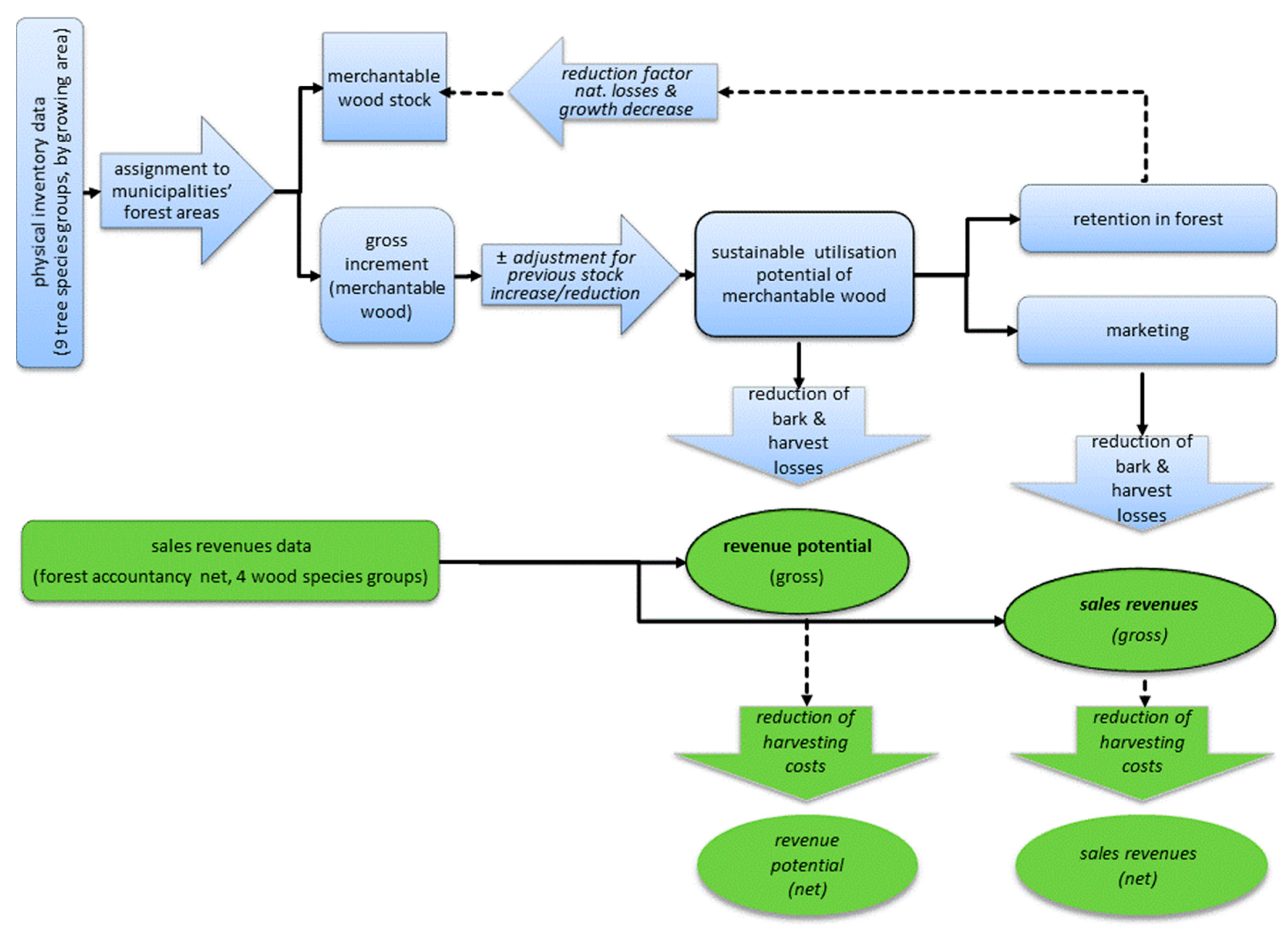In terms of spatial resolution, these are subdivided into 82 German forest growth areas [47]. Annual increment is available both in units of standing volume and harvested volume. We use the standing volume data, which is later also needed for the quantification of carbon sequestration. If necessary we calculate the harvested volume by deducting 10% of the volume for bark and another 10% for harvest losses.

The increment data for the tree species groups of the forest growth areas (from the Federal Forest Inventory) are then assigned to the forest areas of the municipalities (which are derived from CORINE land cover data [43]). For this purpose, the forest area of each municipality is computationally divided into nine sub-areas, one for each tree species group, according to their share in the respective forest growth area. Each sub-area is then multiplied by the average per-hectare-increment of the respective tree species group in the corresponding growth area. The result is the annual increment of merchantable wood in each municipality, which is interpreted as the sustainably harvestable volume per year (i.e., we disregard any accumulation or reduction of stocks which might have happened in the past, because no pertinent spatially differentiated data are available).

The increment of the tree species groups is determined by the actual growth conditions in the growing areas. In addition, the current age structure also influences tree growth, as stands between 20 and 60 (−100) years grow significantly faster than younger or older stands [65]. However, information on age classes or the average age of stands is not available with the necessary spatial differentiation: The published inventory data only allow age differentiation for the tree species groups at the level of the federal states, but not at the level of the growing areas or even at the county level, as otherwise the sampling error would escalate. For this reason, our model abstains from a subdivision into age groups. As an implicit consequence it uses the actual average age of the tree species in the growth areas. For the interpretation of results this is only relevant if calculations are based on scenarios that would significantly change the current age structure (e.g., afforestation scenarios); in such cases, the results would have to be interpreted as long-term effects. For scenarios without an immediate change in the given age structure (e.g., set-aside of forests), this limitation is not relevant.

2.2.2. Valuation

The question of an adequate economic valuation concept for timber seems more obvious than it is. Timber production is the only ecosystem service considered here that provides private goods. These are traded on markets and thus have market prices. It seems obvious to use these prices for valuation purposes. However, market prices differ conceptually from the welfare measures used to value other forest ecosystem services which have characteristics of public goods. In particular, marginal prices do not include consumer (or producer) surplus; they are therefore not fully compatible with welfare measures based on the consumer surplus concept [11]. Differences also exist in terms of property rights: A priori, timber is owned by the forest enterprises, whereas public goods are not. Nevertheless, these differences do not preclude the use of a price-based valuation concept for timber—they only preclude netting prices with surplus-based welfare measures and/or interpreting value relations between different services in absolute terms. In contrast, it is unproblematic to interpret regional patterns of these value relations and their possible changes. Since this is the only objective in the present context (see above), the valuation of timber production as a FES can follow a price-based concept here.

For this purpose, revenue data are available from the federal Forest Accountancy Network (TBN) [66], which are differentiated according to the four wood species groups spruce (comprising spruce, fir, and Douglas fir), pine (comprising pine and larch), beech (comprising beech and other broadleaves except oak), and oak. These are area-weighted roadside price averages which were realized within one year by state, communal, and private forest enterprises; self-sourced firewood is proportionally included here.

Table 1. Timber revenues by tree species group, weighted by type of ownership and share of self-sourced firewood (reference year = 2016).

Wood Species Group	Spruce	Pine	Beech	Oak	Total
Gross revenue (€/m3)	82.86	61.09	61.30	87.05	73.52
net of harvesting costs (€/m3)	39.64	27.76	25.88	49.83	34.26

Data source: forestry accounting results 2016 [66].

shows these averages for the year 2016.

For the present valuation purpose, the gross revenues are relevant. They comprise the income of the forest enterprises on the one hand and harvesting costs on the other, both of which are financed by the ecosystem service “timber production”. Since harvesting costs generate income for other parts of the economy, both kinds of income have to be included, in order to capture the benefits to the national economy as a whole. Accordingly, we first subtract bark and harvest losses from the sustainably harvestable volume established above, and then multiply it by the gross revenues. The result is the gross revenue potential in the municipalities (in € per year).

Furthermore, it can be asked whether additional situational characteristics of forests should be taken into account for the valuation. These could be, in particular, the distances between forests and the processing sites for raw wood, including the transport costs incurred. In practice, this seems hardly possible, as this would require spatially differentiated prices and/or comprehensive mapping of transport routes to the respective wood processors (for all wood assortments produced), which are not available in this differentiation. Moreover, it might not make much sense, since the same argument applies to transport costs as to timber harvesting costs: transport costs, too, are ultimately financed by the ecosystem service timber production and generate income, i.e., benefit the national economy elsewhere. Therefore, we do not subtract transport costs from the gross revenue potential.

The valuation based on revenue potential does not differentiate between whether the usable increment is actually harvested or not. In order to enable (gradual or total) harvesting restrictions in both commercial forests and nature conservation areas, the sustainable use potential can therefore be divided in a further step into a marketed portion and a portion that remains in the forest. The marketed portion is then valued at the gross proceeds from Table 1 (again after subtracting bark and harvesting losses), the non-marketed share at zero €/m³. These portions remain variable so that the model can be used for different forest utilization scenarios. The current situation is approximated by a reference scenario that is based on actual harvests in the status quo according to the Federal Forest Inventory. It reflects the proportion of harvest restrictions by protected areas (in their given spatial distribution) and other harvest restrictions.

Figure 1 shows a recap of our procedure for valuing timber production as a FES.

2.3. Carbon Sequestration

The global climate protection service of forests is based on the removal of carbon from the atmosphere through photosynthesis and on its storage, at first in the ecosystem [41]. Second, the storage can be continued in wood products after harvesting [67]; depending on the type of use, the use of wood may also replace emission-intensive products and processes [68]. Altogether this reduces the proportion of climate-damaging greenhouse gases in the Earth’s atmosphere, which would otherwise contribute to further global warming. The goal of the valuation is to determine the monetary benefit of this primary and secondary mitigation effect for German society.

2.3.1. Quantification

First of all, it must be determined whether only carbon sequestration (i.e., the carbon captured annually by forests) should be considered as a climate protection service, or also carbon storage (i.e., the protection of historically accumulated carbon which is stored in various carbon pools). Although there are arguments for both [69], we only consider the annual sequestration here in order to avoid double counting, since the carbon pools do not contain anything else than the sequestration of the previous years. Clarification is also needed as to whether gross or net sequestration should be recorded for quantification, i.e., whether or not harvests should be subtracted from the annual increment. As we do not restrict our view to the carbon pools in the ecosystem only but include harvested wood products (HWP) and substitution effects (i.e., carbon displacement), too, we have to consider the carbon fluxes between pools, again to avoid double counting. This implies a net concept of sequestration (i.e., subtracting all carbon releases from the pools, such as harvests).

Practically, we determine the respective net sequestration in all cases by calculating stock changes. For this purpose, our model distinguishes three categories: the forest pools, the HWP pool and substitution. Among the forest pools we account for changes in living aboveground tree biomass only (merchantable wood >7 cm diameter, brushwood <7 cm and needles). We do not include changes in deadwood, roots, soils, and litter, because the underlying exchange processes (especially root decomposition) are largely unexplored; therefore, the influence of harvests as well as calamities on these pools cannot be quantified with sufficient accuracy using literature references. This omission tends to underestimate the sequestration capacity within forests; empirical results indicate an increase of C-reserves in the mineral soil over time [70] (whereas the changes were insignificant in the litter layer).

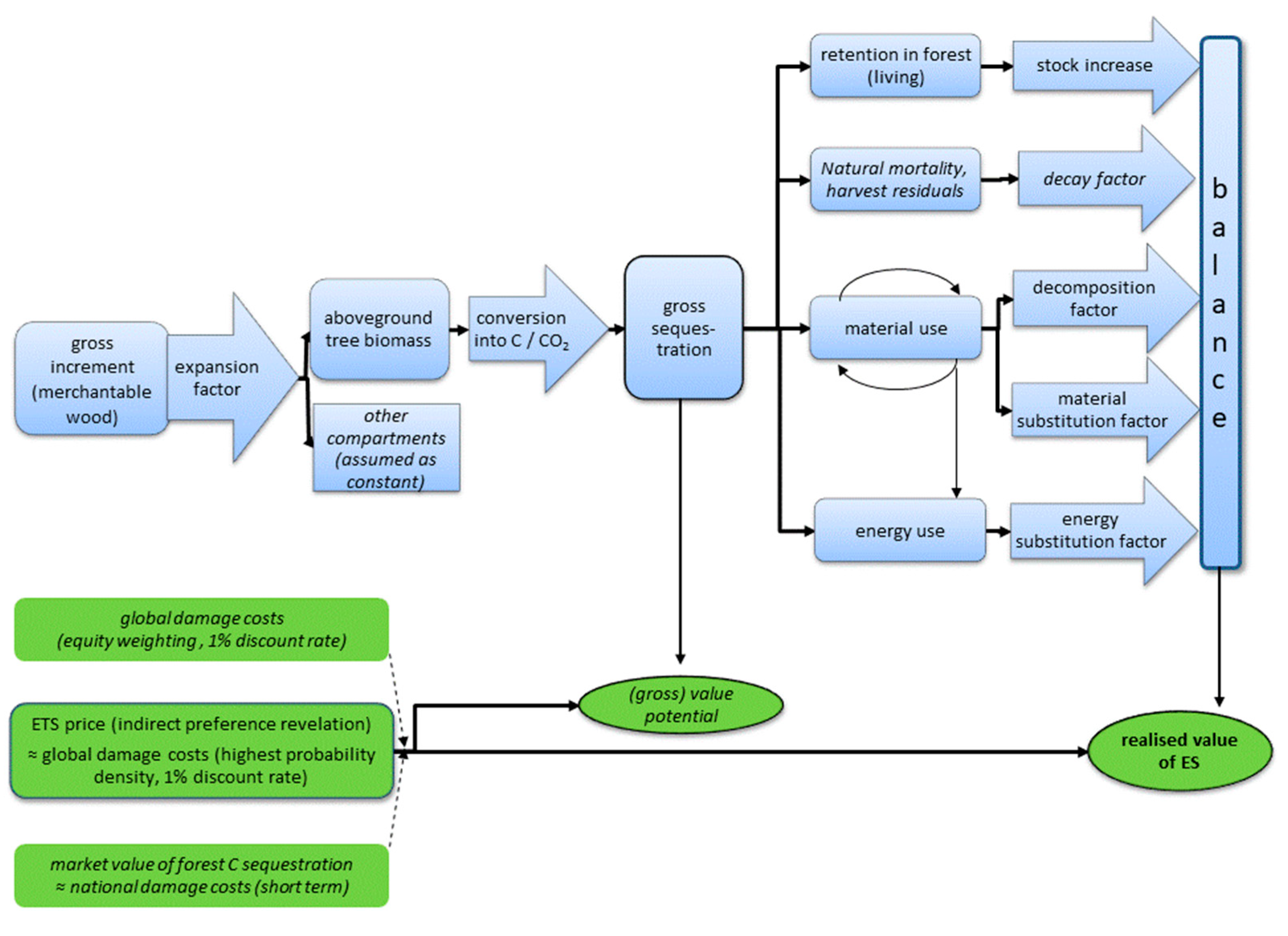
For quantifying the carbon dioxide contained in the aboveground biomass, we proceed from the standing volume of merchantable timber which has already been established in the timber production module of the model (see above). The volume of brushwood and needles is calculated using the tree-specific expansion factors given in [71]. In order to convert volume to mass, we use the IPCC’s conversion factors [72], which also distinguish between tree species and between merchantable and other wood. The average C content is assumed to be 50% of the mass for all tree species; finally, the conversion factor from C to CO₂ is 3.67, according to the ratio of the respective molar masses.

For determining the changes in the HWP pool we apply the “Climate Calculator” of the German Forestry Council [73,74]. After deducting 10% each for bark and harvest losses, this calculation tool distributes the remaining wood volume to different material and non-material uses, depending on tree species and diameter, and assigns them corresponding lifetimes, with input data that are derived from empirical averages in Germany [74]. Data on the distribution of the harvested trees’ diameters was derived from the average distribution of harvesting rates per age class and tree species in Germany [64].

Both material and energy substitution effects follow the assumptions of the Climate Calculator, too. It assumes that for each ton of C in material use of wood, 1.5 t C in non-wood products are replaced, according to [75]. Material substitution is only assumed for products with a medium and long lifetime as well as for wood products of the packaging industry, excluding paper and paperboard. For the energetic substitution, a displacement factor of 0.67 t C/t C is applied [76,77] (indicating that one ton of C in the energy use of wood replaces 0.67 tons of C in alternative fuels). All wood used for energy purposes is taken into account here, including firewood from forests, industrial waste wood and other waste wood which is not further recycled. Generally, we consider the assumptions of the Climate Calculator concerning substitution relatively optimistic [78]; they might possibly lead to an overestimation (which then counterbalances the underestimation of underground sequestration mentioned above). However, it must be borne in mind that determining substitution from an ex ante perspective is only possible in a relatively rough way. Carbon displacement factors are only available for individual products, which have to be determined with the help of life cycle assessments in an elaborate process; in addition, production processes and the energy mix in the economy are subject to constant change.

2.3.2. Valuation

As in the case of quantification, it is not immediately self-evident which approach to choose for valuation. Willingness-to-pay analyses appear theoretically coherent, and some pertinent case studies are also available for Germany [79,80,81,82,83,84,85,86,87,88,89]; however, results vary so strongly that they do not allow deriving a reliable average value for emission reductions (or equivalently, for carbon sequestration). Social costs of carbon also appear acceptable in theory, but their results vary widely again [90], they require a wealth of assumptions [91] and are therefore susceptible to manipulation. Damage avoidance costs are less consistent with a demand side valuation as they simulate supply curves; they again rely on a plethora of underlying assumptions [92], and they raise logical problems in the presence of negative avoidance costs. Finally, although market prices realized in mandatory Emission Trading Systems (ETS) are theoretically less suitable as demand indicators and therefore do not provide accurate estimates of the benefits of carbon sequestration, they can still be interpreted (in a democratic system) as indirect manifestations of climate protection demand; and most importantly, they are based solely on observation. (For a more detailed discussion of carbon valuation issues, see [93,94]).

We have therefore based our valuation on market prices [(i.e., on the average EU-ETS price for the second half of 2018; this was €19.49 per tonne of CO2 [95]). This primarily reflects a scarcity price for emission rights, which is the economic result of diverse and complex political processes [96,97]. Since this policy is democratically founded and is also subject to democratic control, the EU-ETS price can also be interpreted in a very broad sense as an indirect preference revelation by society. As an estimate of global damage costs or a rent-based welfare measure, it contains underestimation tendencies and thus serves a rather cautious valuation. However, a market price of around €20/t CO₂ is only slightly below the global damage cost estimate with the highest probability density (i.e., around €22/t CO₂), as estimated in a meta-analysis of existing damage cost assessments for an interest rate of 1% [98]. Two other important aspects are that, among the valuation approaches considered, market prices are least influenced by assumptions and subjective norms; moreover, they come closest to the income effects that could result from a (hypothetical) commercialization of carbon sequestration by forests in a mandatory trading system.

Figure 2 summarizes the procedure for quantifying and valuing the climate protection service due to carbon sequestration.

2.4. Recreation of Local Residents

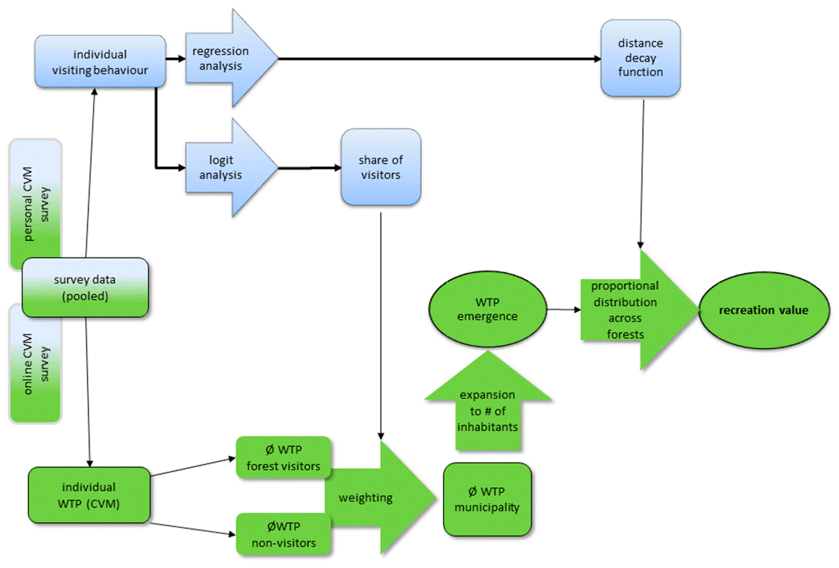
This module aims to assess the benefits that forest visitors receive from everyday forest visits near their place of residence. Forest recreation is a public good in Germany, as the Federal Forest Act generally allows anyone to enter all forests for recreational purposes free of charge [99]. Therefore, we capture the recreational service conceptually via the right of access to those forests people actually visit, and its annual value via their willingness to pay (WTP) for a hypothetical entrance ticket that allows them to visit every forest in their vicinity for one year. Forest visits on the occasion of holiday journeys are thus excluded. Our main data source is the original data set from a fairly recent survey on this issue, which is representative for the German population [100]. It contains the respondents’ individual place of residence (as postal code), their visit frequencies in all forests in their vicinity (defined as total number of forest visits during the last 12 months in their free time, which were released without an overnight stay away from home), the distance to the last forest visited (in km, as estimated by the respondents), answers to several WTP questions based on the Contingent Valuation Method (CVM) in a “consequential open ended” design [101,102] (which elicited the individual WTP per person per year for a hypothetical annual entrance ticket to all forests in their vicinity), and some socioeconomic variables. These variables which are available from the survey are supplemented by data of the municipalities which originate from regional statistics information (e.g., forest characteristics, number of inhabitants and average income).

2.4.1. Quantification

First, we estimate the respondents’ individual probability of being a forest visitor (defined as making at least one local forest visit in a year) by means of a logit regression, using the visit frequency data as an input. Because this regression is to be used later for simulating the visitor proportions in the municipalities, only those variables that are available at the municipality level can be used as potential explanatory variables here. The explanatory variables that turn out to be significant are the respondents’ net household income as well as the number of inhabitants and the percentage of forest area in their residential municipality, which all have a positive influence on visit probability.

Table 2. Logit regression of the probability of being a forest visitor ^1.

	Coefficient	Standard Error	z Value
Net household income (€/month)	0.000290	0.000000292	4.89 ***
Forest share at residence (%)	1.504872	0.0000593	3.79 ***
Number of inhabitants (n)	0.000000531	0.1726439	1.82 *
Constant	0.4848901	0.3973568	2.81 ***

¹ LR Χ² = 41.76 ***; Log-likelihood = −739.60, pseudo–R² = 0.0275; N = 1624. Number of asterisks indicates significance level (90% *, 99% ***). Data source: [100].

shows the results.

We then use this relationship to calculate the share of forest visitors in each of the 11,533 municipalities, interpreting visit probabilities as visitor shares and replacing individual income with average income in each municipality. This results in a range of visitor shares between 77.65% and 97.20% in the municipalities, with a mean of 87.63% (note that this is an estimate of visitor shares on average across municipalities, not a population average). Multiplied by the number of inhabitants, this gives the number of visitors in a municipality.

2.4.2. Valuation

For valuation, we first calculate the mean WTP in each municipality and aggregate it to the total number of this municipality’s inhabitants; then we distribute the aggregated WTP across the surrounding forests.

As to the first step, the mean WTP per municipality is calculated simply as the weighted average of the WTP of visitors and non-visitors, using Germany-wide WTP means for both groups (i.e., 32.27 € per person per year for visitors, and 11.50 €/p/a for non-visitors; recalculated from [100]). Note that the average “non-visitor” also has a positive WTP for forest visits; this is partly due to option values and partly due to the fact that some non-visitors do visit forests, but less frequently than once per year. The weighted WTP average of each municipality is then multiplied by the number of its inhabitants, which gives the aggregate WTP in each municipality.

In a second step, the aggregate WTP of each municipality must be distributed over those forests that are visited by the residents of this municipality. For this purpose, we assume that the distribution of WTP is strictly proportional to the distribution of visits. In order to determine the latter, we estimate a distance decay function, again using the original data from [100] that include the individual distances to the last visited forest. As estimating the distance decay function directly from the observed visits would yield biased results (p. 41 of [93]), we first create a cumulative frequency distribution by successively adding the visit frequencies from each distance. Inverting this distribution results in a “survival curve” that describes how many visits remain up to a given distance. It can be fitted by a negative exponential function; for the present purpose, the standard biexponential function,

$$n=\alpha +\beta ·{\mathrm{e}}^{-\gamma D}+\delta ·{\mathrm{e}}^{-\eta D}+\epsilon$$

(1)

is applied that yields an almost perfect fit (R² > 0.99; n is number of visits, D is distance, Greek letters are parameters, except of ε which is the error term). Its first derivative [103],

$$f^{\prime }\left(D\right)=\beta \gamma {\mathrm{e}}^{-\gamma D}+\delta \eta {\mathrm{e}}^{-\eta D}$$

(2)

gives the sought-after distance decay function, which shows the number of visits from a given distance.

Table 3. Parameter estimates for “survival curve” (1) and distance decay function (2) (R² = 0.9973).

Parameter	Estimate	Standard Error
α	1.0186282	0.283
β	141.36847	6.080
γ	0.8234692	0.060
δ	40.783303	3.197
η	0.1142546	0.009

Data source: [100].

presents the respective parameter estimates.

The distance decay function is then applied to distribute the aggregate WTP from each municipality across the surrounding forests. The basic principle is simple: We determine what proportion of a municipality’s forest visits (and thus of its WTP) is allocated to the forests in that municipality and distribute the remaining proportion to forests beyond the municipality’s boundaries, proportionally to the respective distances. Technically, we first determine the shortest distance between the center of each municipality and the closest border of each forest. To limit the computational effort, this search is restricted to forests within a configurable maximum distance (here 50 km, which covers more than 99% of all visits according to Formula (1)). The next step is to apply the distance decay function for calculating the number of visits from the municipality to each forest. These visits are summed up and normalized to 100%; the result shows what percentage of the municipality’s visits is allocated to each forest. Subsequently, the percentages are multiplied by the aggregated WTP of the municipality. The WTP of all municipalities is finally added up for each forest area; this gives the aggregated recreational value of that forest area, which is then assigned to the respective county.

Figure 3 summarizes how the recreation service was quantified and valued.

2.5. Services for Nature Protection and Landscape Amenity

The aim of this module is to identify the benefits that people derive from the cultural services provided by forests for biodiversity, nature, and landscape protection. 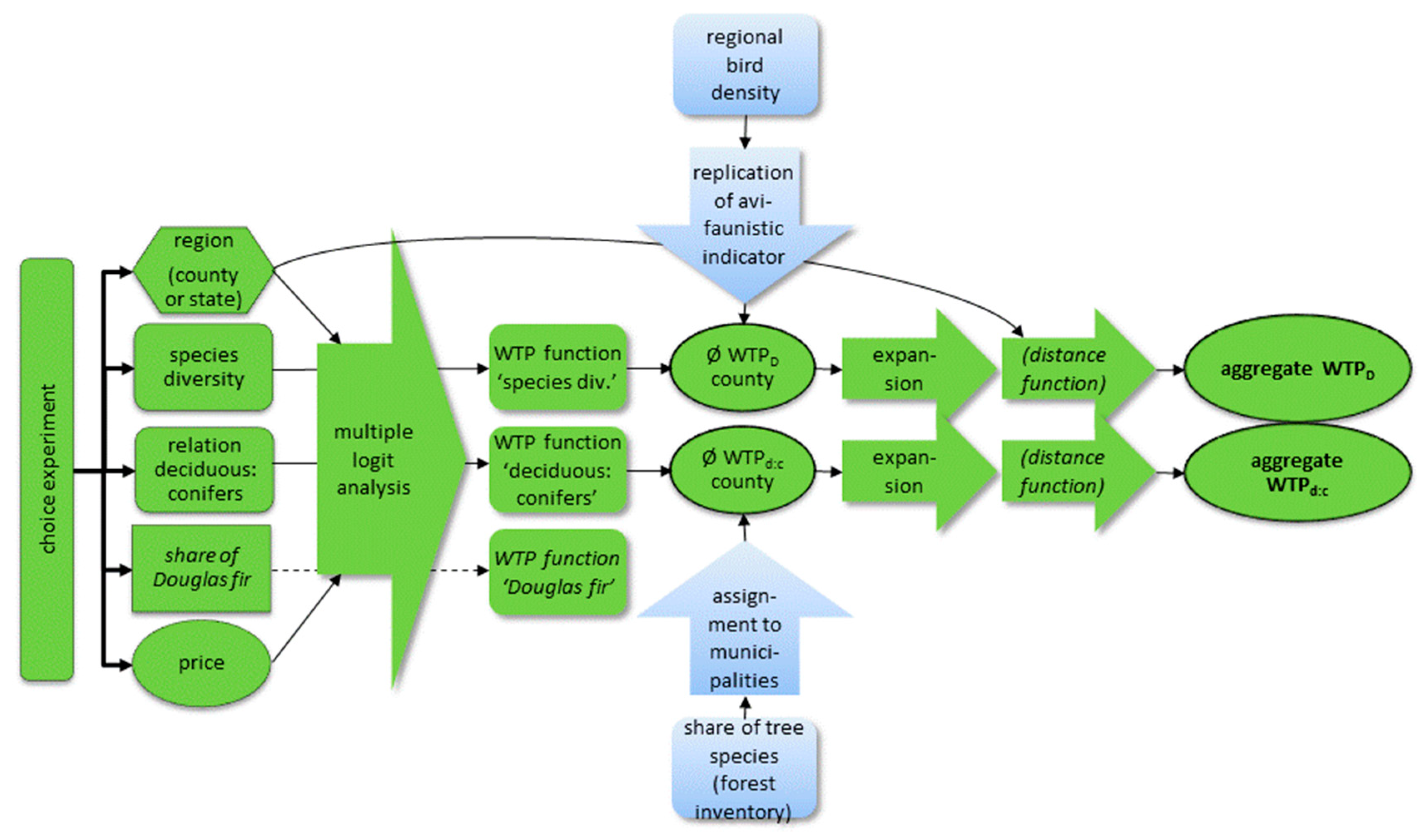Since these are too complex to be measured directly, the valuation focuses on appropriate indicators instead—without claiming that this would cover all relevant aspects of biodiversity protection (one such omission concerns the aspect of ecosystem vulnerability, to give just one example [104]). We opted for avifaunistic diversity and tree species composition as indicators, which are both relevant and understandable to laypersons, politically connectable, and for which basic data are available in Germany. In order to elicit the citizens’ preferences for changes within forests as measured by these indicators, a separate representative survey was conducted that included, inter alia, a choice experiment (CE) on these issues. This survey is detailed in [93]; in the present article we restrict ourselves to applying the valuation results obtained to determine spatial benefit distributions.

2.5.1. Quantification and Valuation of the Forest Biodiversity Indicator

Forest biodiversity is assessed using the Federal Nature Protection Agency’s avifaunistic indicator on “Species Conservation and Landscape Quality” [50,51], which is also used and regularly updated in the German Sustainable Development Strategy [53]. The indicator is composed of six sub-indices, including one for forests. This sub-index “forests” measures the occurrence and population densities of eleven forest-typical bird species. Since these bird species have specific habitat requirements and the respective habitats in turn harbor other species, the index also points to biodiversity and habitat quality in general [50]. An index value of 100 describes a predefined population target value derived from a presumed state in the past; index values below 100 can be interpreted as the degree of target achievement in percent.

Unfortunately, this indicator as well as its sub-indices are only available for Germany as a whole, but not in any spatial disaggregation. We therefore had to reconstruct the spatial distribution of the forests sub-index at county level, using the Atlas of German Breeding Birds as the data source [54]. These data describe the abundance of breeding pairs of those eleven bird species the sub-index is composed of the basic spatial unit is a topographic map at a scale of 1:25,000 (i.e., a map cell with an area of approximately 126 km²). Abundance is not reported in absolute numbers in the data but is assigned to one of 10 abundance classes for each cell.

For each bird species, we record the maximum abundance class that could occur in any of the cells as well as the abundance class that it actually reaches in each cell and express the latter as a fraction of the former. Subsequently, we calculate the average of these fractions across all bird species for each cell (accounting only those bird species that can actually occur in the respective cell; outside the range of a species, we assume that its habitat requirements are not fulfilled there and exclude it from the calculation). Finally, we calculate the area-weighted mean value for each county from the results of the individual cells and rescale it into percentage values in order to be directly comparable with the original indicator. (For more details see [105]).

With regard to valuation, we used the bird diversity index as an attribute in one of the choice experiments reported in [93]. More specifically, we established the respondents’ WTP for a marginal change of the status quo of forest biodiversity in their home county, explaining to them the general interpretation of the forests sub-index as a measure of species diversity, and its current average value in Germany (i.e., 85 index points at the time of the survey [52]). This resulted in an average WTP of €1.54 per household per year for a diversity increase by one index point, with 95% confidence intervals between €1.12 and €1.96 [93].

As our spatial reconstruction of the forest diversity index corresponds exactly to the description in the choice experiment, the result of the latter can be applied directly, by simply multiplying any marginal change in the diversity index with the associated mean WTP. However, two caveats should be noted. First, the choice experiment only identified the benefits of increasing forest biodiversity within the respondents’ respective home counties; benefits in other counties were not captured. However, there is evidence from the survey that such benefits do exist. As a consequence, our valuation results tend to underestimate aggregate benefits for the country as a whole. Second, the valuation results are only valid for marginal biodiversity changes around the current status quo but should not be linearly extrapolated for calculating some “overall value of forest biodiversity”. The reason for this is that marginal utility most probably increases with decreasing diversity and may become infinite once essential elements of diversity are threatened. Extrapolating the results to calculate an “overall value of forest biodiversity” would thus cause “a serious underestimate of infinity” (p. 58 of [106]).

2.5.2. Quantification and Valuation of Tree Species Composition

Tree species composition is an important element of the beauty of a forest landscape. Moreover, tree species composition is one of the few landscape-shaping characteristics of forests that is suitable for large scale analysis. It also plays an important role in the forest policy debate in Germany, especially with regard to increasing the proportion of deciduous trees [107,108] and the controversial cultivation of non-native tree species [109]. Both aspects have therefore been included as attributes in the choice experiment mentioned above [93]. Here we present valuation results for changes in the share of deciduous trees (in contrast, the results on non-native tree species are omitted because they turned out to be contradictory and not very reliable [93]).

To quantify the share of deciduous trees in the municipalities, the analysis of the Federal Forest Inventory data by growth areas is used, as already described for the module timber production. From this data, virtual pure stand areas in the municipalities are available, which are subdivided according to nine tree species groups. From this, the ratio of deciduous and coniferous trees in the municipalities is calculated.

Estimates of the individual WTP for different proportions of deciduous trees originate from the choice experiment in [93]. Specifically, the choice experiment provides the annual WTP for deciduous tree proportions of 5, 25, 75, and 95% in the respondents’ respective home county (with 45% as the reference category).

Table 4. Willingness to pay (WTP) for different shares of deciduous trees (DT_v) in € per household and year, depending on actual share of deciduous trees in home county (DT_a), according to [93].

Valued Share (DTv)	All Respondents	Actual Share (DTa) in Home County 1
		25%	50%	75%	95%
5%	−136.93	−201.56	−138.23	−123.39	−131.48
25%	−75.75	−65.11	−81.10	−72.52	−37.74
75%	+27.61	−13.18	+11.07	+79.85	+89.13
95%	−93.73	−125.74	−135.25	−35.02	+59.02
Number of respondents	1423	356	476	511	80

¹ as estimated by respondents. 35 respondents from counties with only 5% deciduous trees excluded (due to insignificant WTP estimates caused by low number of observations). Source: [93].

shows these WTP data for all respondents (second column). Since there is evidence that people’s landscape preferences are influenced by the conditions in their place of origin [110,111,112], the table also shows the respective WTP of subgroups differentiated according to the actual proportion of deciduous trees (DT_a) in the home county, as estimated by the respondents (last four columns).

Table 4 shows that WTP is non-linearly correlated with the share of deciduous trees to be valued. It can be fitted by a quadratic smoothing function,

$$WTP=\alpha +\beta ·D{T}_v+\gamma ·D{T}_{v}2+\epsilon$$

(3)

where WTP is willingness to pay in €/household/a, DT_v is the share of deciduous trees to be valued in percent, αβγ are parameters to be estimated, and ε is the error term.

Table 5. Parameters of function (3) for estimating WTP for different shares of deciduous trees (DT_a).

Share of DTa in Home County	α	β	γ	R2	R2adjusted	Apex
25%	−250.3256	9.781637	−0.0889298	99.8	99.4	55.0%
50%	−194.2529	7.725761	−0.0726571	78.6	35.7	53.2%
75%	−180.7700	7.388414	−0.0591943	81.8	45.4	62.4%
95%	−168.0398	6.639325	−0.0442340	99.4	98.3	75.1%
All respondents	−189.0151	7.373184	−0.0651876	83.5	50.6	56.6%

Data source: Table 4.

shows the parameter estimates, again for all respondents together (bottom line) as well as differentiated by actual deciduous tree share in the country of origin (previous lines). The last column shows the apex of each resulting parabola, which is calculated from the zero of the first derivative [103],

$$\frac{\beta }{2\left(-\gamma \right)}$$

(4)

It can be interpreted as the computational optimum of the deciduous tree proportion, which obviously increases the more a respondent’s environment is characterized by deciduous trees.

Table 5 now provides the basic tool for valuing changes in the proportion of deciduous trees: After calculating the WTP for the actual and the targeted share (DT_a and DT_v, respectively), the former is subtracted from the latter. This difference is the WTP for the change in the proportion of deciduous trees. Multiplied by the number of households, this finally gives the aggregated willingness to pay for a change in the share of deciduous trees in a municipality. In order to allow for deciduous tree shares between the point estimates given in the table, the values of the given parameters are linearly interpolated, if necessary.

Note that tree age had to be disregarded in our model due to the lack of suitable input data, as explained above. This implies that the procedure described here reflects long-term effects of a change in tree species composition. When gauging short-term effects, it should be borne in mind that a change in tree species practically starts with young trees, which may be valued differently from old-growth stands or from the existing age mix. However, taking this into account would not only require a forest growth simulator in combination with more differentiated quantitative input data, but also differentiated valuation data that, in addition to the tree species mix, also take into account different ages of the admixed trees.

As a brief summary, Figure 4 schematically shows the procedure for quantifying and valuing the services for nature protection and landscape amenity.

3. Results

The following section presents aggregated benefit estimates for the entire country, validates these by a comparison to reference values, and subsequently shows the spatial distribution of the benefits.

3.1. Annual Benefits of Timber Production

According to our modelling results, the gross timber revenue potential in Germany amounts to a total of €7.1 billion/a (i.e., the sustainably harvestable increment of merchantable timber after deduction of bark and harvesting losses).

For comparison with a suitable reference we proceed as follows. Conceptually, the sum of the revenue potentials of all municipalities corresponds to a large extent to the “production value of biological production” from the extended forestry accounts (cf. [113]) resp. the monetarily valued “net annual increment” from the national forest accounts [114] as well as the European Forest Accounts [115]. However, the valuation in these accounts is not based on gross revenues, but on revenues free of harvesting costs. We therefore conducted a control calculation on the basis of harvesting cost-free revenues with price data from 2016. It actually showed good agreement between the forest accounts and the revenue estimates of the model summed up across all municipalities: After accounting for the different input data of both sources (in terms of physical increment, forest area and their respective accessibility) and some definitional differences in detail, the aggregated estimate of our model exceeded the corresponding figure from the forest accounts by less than 1%.

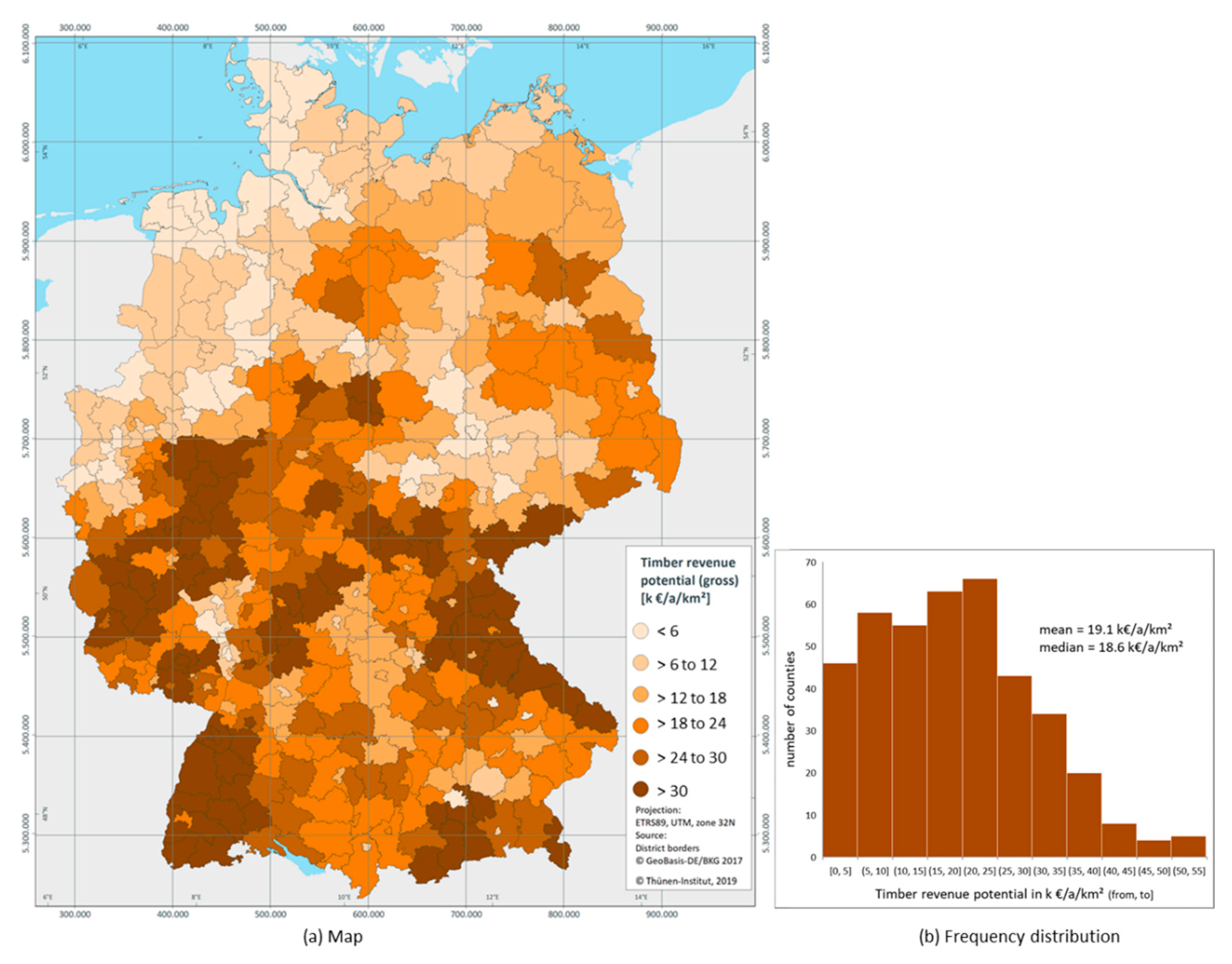
Figure 5 shows the regional distribution of the annual gross revenue potentials based on the timber revenues of the year 2016, aggregated at county level, as well as the associated frequency distribution (in k€/a/km²).

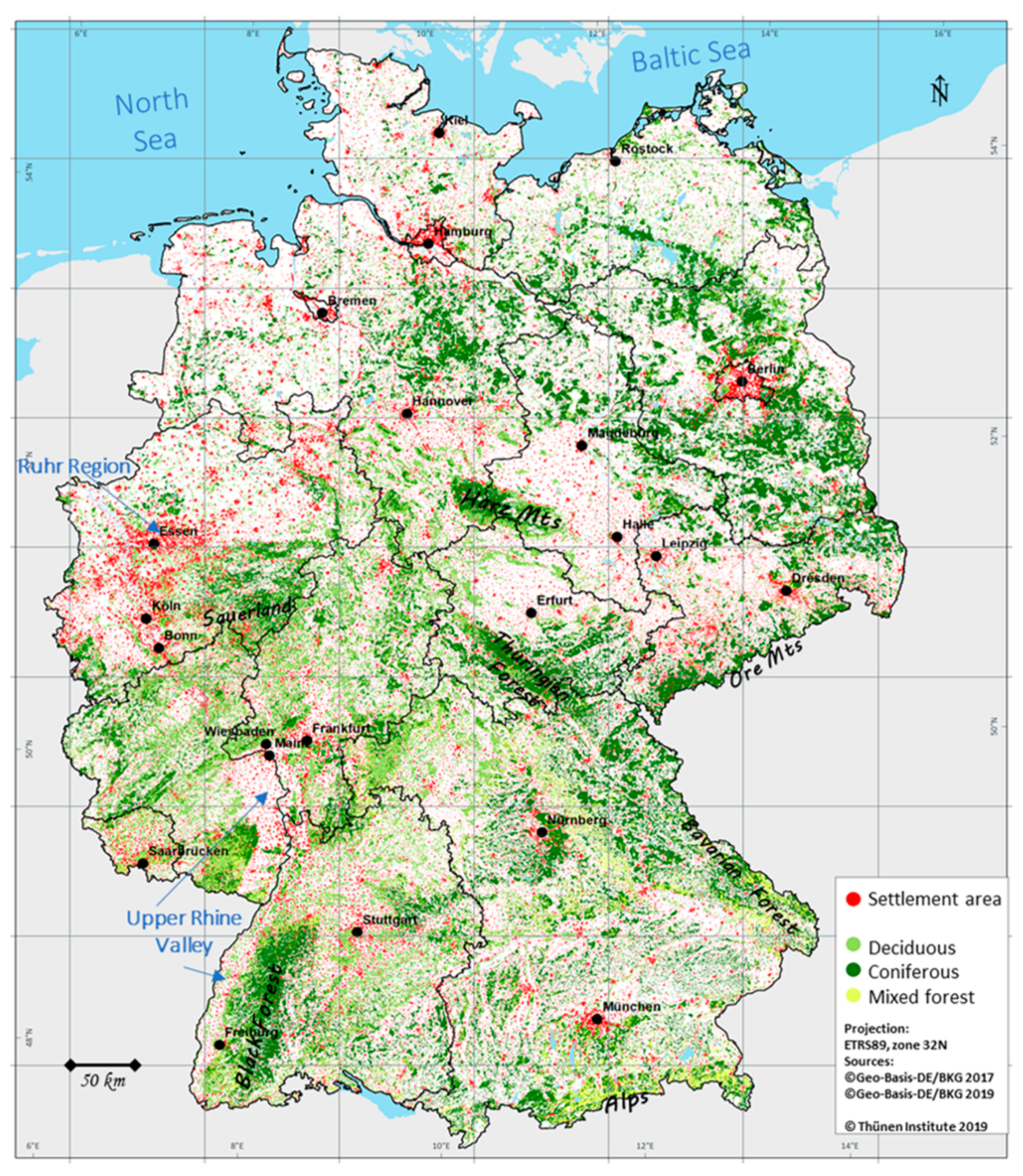
The regional distribution reflects the share of tree species in the forest growth areas as well as their increment and their respective timber prices on the one hand; on the other hand, the aggregated values are also influenced by the different forest areas of the counties. The Bavarian Forest (Bayerischer Wald) in the southeast, the Black Forest (Schwarzwald) in the southwest, the Sauerland in the west and the Ore Mountains (Erzgebirge) further east stand out with particularly high revenue potentials, as these areas are both densely forested and have a high proportion of financially productive tree species (for locating the mentioned areas see Appendix A). In the pine-dominated north-east, the revenue potential per hectare is lower; high revenue potentials there result from the fact that the areas are densely forested. The frequency distribution turns out to be asymmetric but mean and median are quite close to each other (note that this is the mean across all counties, rather than a population mean for Germany as a whole). About one quarter of all counties—predominantly in the north—have revenue potentials below 10 k€/a/km²; the value range, however, extends to almost 52 k€/a/km². The mean value of the revenue potential of all counties is almost 20 k€/a/km²; in absolute terms this is 16.8 million €/a per county.

The valuation based on the revenue potential does not consider whether the usable increment is actually harvested or not. Therefore, we additionally simulate a reference variant in order to reflect the value of current timber harvests. It is based on the actual harvests in the status quo (according to the Federal Forest Inventory 2012) as well as the amount of harvest limitations due to protected areas (in their given spatial distribution) and other renunciations of timber use. In total, the gross revenues calculated in this simulation amount to 6.0 billion €/a, which is 14.8% (1.1 billion €/a) below the sustainably usable potential.

3.2. Annual Benefits of Carbon Sequestration

Summed across all municipalities, the physical carbon mitigation amounts to 108 million t CO₂/a under current harvests according to our model results. Evaluated at an EU-ETS price of €19.49 per ton CO₂ in the second half of 2018 this translates to an aggregate benefit of 2.1 billion €/a.

To check the result, the physical carbon mitigation calculated by the model was compared, on the one hand, with the results of the German National Inventory Report (NIR) [116] (annual average from 2002 to 2012), and, on the other hand, with the values calculated for Germany as a whole by Schluhe et al. [74] using the Climate Calculator. Unfortunately, direct comparisons are not possible in either case, as both the NIR and the Climate Calculator only partially cover the carbon pools considered in our model: The NIR includes underground biomass in addition to the compartments considered here, but does not quantify any substitution, which, however, is responsible for most of the carbon mitigation according to both the present model and the Climate Calculator. On the other hand, Schluhe et al. [74] include substitution, but their data do not contain non-merchantable wood and are also limited to the respective main stands (moreover, their results are extrapolated from a sample that comprises only one thousandth of the forest area). In addition, there are further definitional differences in each case, which also lead to quite considerable differences between the two reference sources (for a detailed discussion see [74]). Due to these limitations, only rather rough comparisons are possible. If this is taken into account, our results appear plausible in comparison to the two aforementioned sources: Once the effects of various definitional differences are factored out, our results are about 6.6% higher than the mitigation per hectare calculated by Schluhe et al. [74]; compared to the NIR [116], they are about 7.4% higher in those storage compartments included there. The primary cause for the remaining differences is likely to be found in the respective estimates of the amount of wood removals, which differ considerably in Germany [117,118]. Given that our model does not cover all storage compartments and neglects underground carbon storage in particular, the remaining overestimation of the physical sequestration service—if it exists at all—is likely to be negligible (and, in any case, it takes a back seat relative to the many uncertainties inherent in the valuation of carbon).

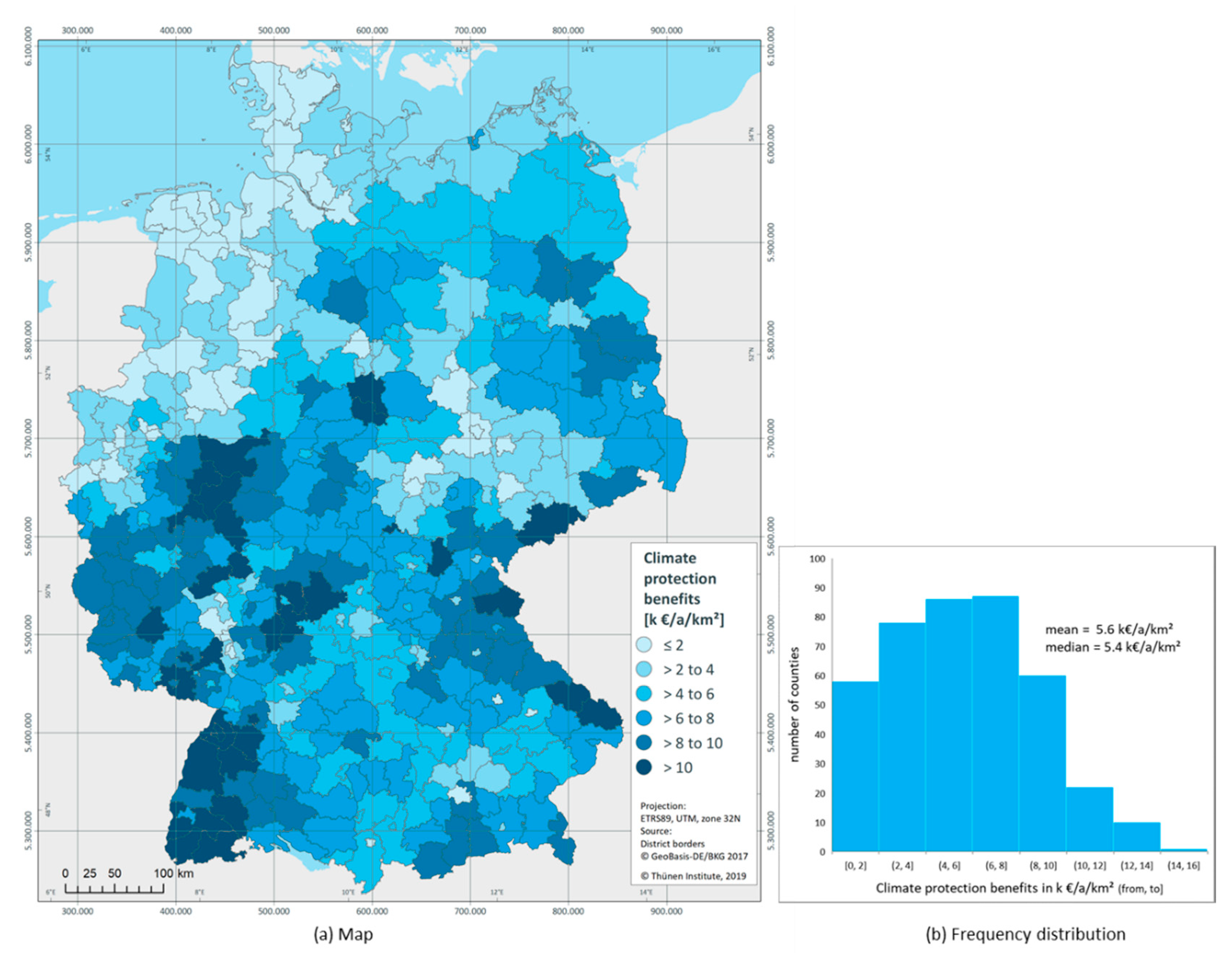
Figure 6 shows the spatial distribution of the climate protection benefits in the delimitation used here, aggregated to counties, and the corresponding frequency distribution (again in k€/a/km²).

The spatial distribution pattern is very similar to that of the raw wood potential. This is not surprising, because wherever forests are abundant, there are also high potentials for raw wood production as well as for climate protection services—both are causally related to wood increment. Therefore, the same regional foci emerge for both climate protection and wood production. Differences in the patterns occur because, on the climate protection side, the different carbon densities of the tree species as well as the utilization of their timber play a role; in contrast, there are no price differences between the individual tree species at this point. The frequency distribution is also quite similar to that of the raw wood potentials. In more than a third of the counties, climate protection benefits amount to less than 4 k€/a/km², but the value range extends to 14.5 k€/a/km².

The valuation is based on a reference scenario with a harvesting intensity like today, in which increments exceed harvests. For direct comparability with the volume basis of the timber revenue potential, an alternative scenario is defined in which all sustainably harvestable increments are harvested, i.e., where harvests equal increments. In this scenario, climate protection benefits would be lower by almost €0.2 billion/a, totaling €1.9 billion/a. In other words, a scenario of increasing harvests to the full increment would cost society about €0.2 billion/a in terms of foregone climate protection benefits.

3.3. Annual Benefits of Forest Recreation by Local Residents

Summed across all municipalities, the aggregate benefits of everyday forest recreation (i.e., excluding holiday trips) amount to €2.4 billion/a. This result is obtained after extrapolation to the total population without any deductions (82.8 million inhabitants, including minors). Extrapolated only to the population over 14 years of age (72.6 million people), the result would be 2.1 billion €/a; extrapolated to the adult population (69.3 million people), it would amount to 2.0 billion €/a.

Unfortunately, the result calculated by our model cannot be checked against an independent reference, as a comparable valuation study representative for Germany does not exist. However, a comparison to the original study [100] still makes sense, as it helps to detect possible computational errors and/or statistical problems caused by our approach. Therefore we compared the mean WTP of all municipalities calculated by our model (i.e., €29.70 per person per year) to the population mean estimated in the original data source [100]. The mean value estimated by the model exceeds the latter by only 0.72 €/p/a (2.5%). About one third of the remaining difference is attributable to the above-average WTP of those respondents who did not provide information on the frequency of their visits in the original survey, and thus had to be neglected here. The remaining gap is probably caused by a statistical peculiarity of our model: strictly speaking, it does not estimate the average WTP of all residents of a municipality, but the WTP of a synthetically constructed “average resident”. However, the comparison reveals that the resulting difference is quite small and did not cause a strong bias.

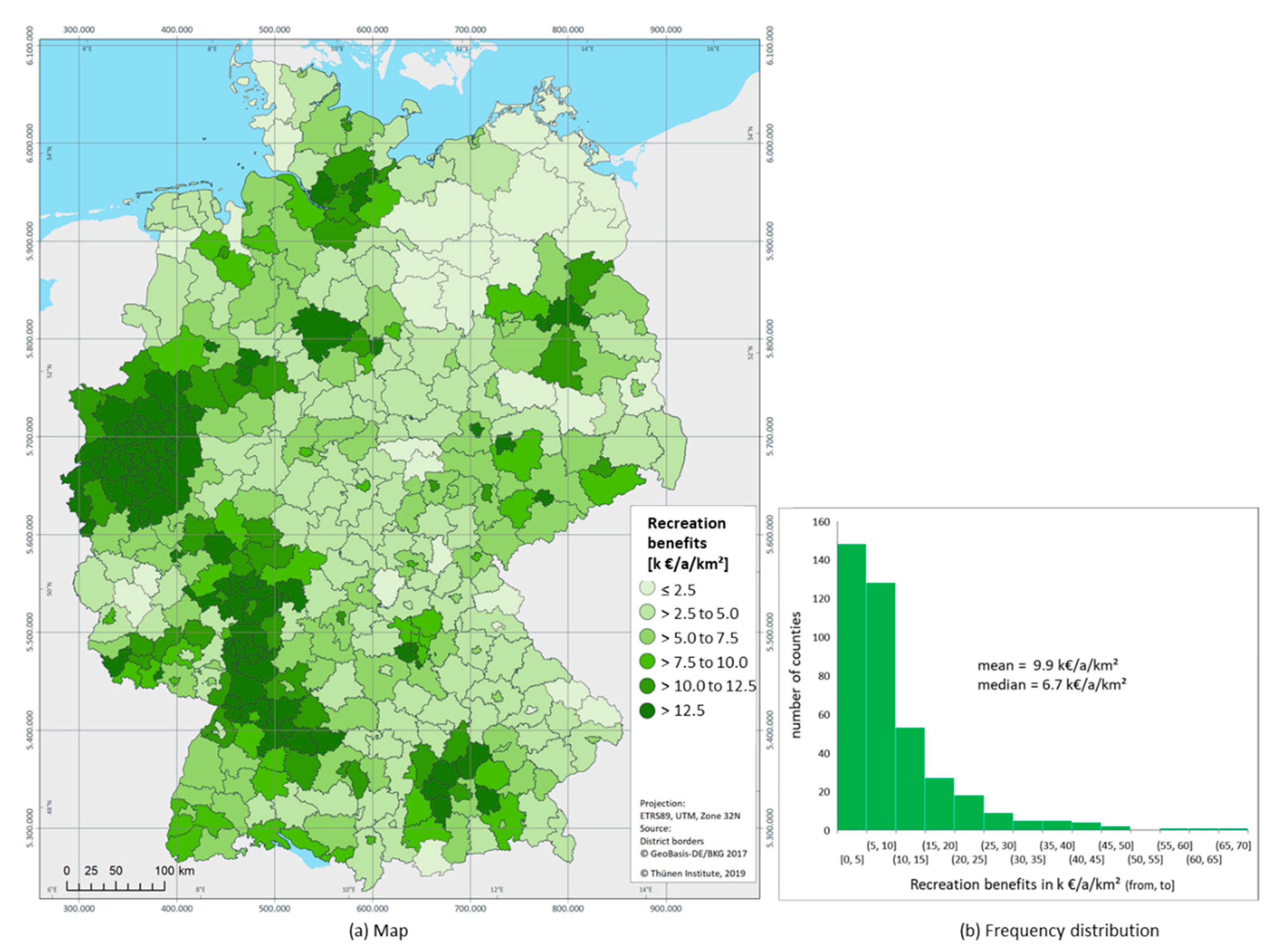
Figure 7 presents the spatial distribution of recreation benefits for local residents, aggregated to counties, and the corresponding frequency distribution, both in k€/a/km².

According to the map (Figure 7), the regions around the densely populated Ruhr Region and the Upper Rhine Valley as well as the large cities (e.g., Hamburg, Hanover, Berlin, and Munich) stand out with particularly high recreation benefits (consult Appendix A for localization of regional names). The WTP of the local population is by no means restricted to the forests within each county, but strongly influences the recreational values of the adjacent counties. This can be seen very clearly in the counties around Berlin, for example. On the other hand, two thirds of the counties have recreation values below 10 k€/a/km². Thus, the frequency distribution of the recreation benefits is strongly skewed to the right; it covers a value range between less than 1 k€/a/km² and more than 68 k€/a/km² (i.e., it is even broader than that of the timber production values), with a mean value across all counties of 9.9 k€/a/km².

The recreational benefits determined here describe the present situation. Changes in value can be calculated by simulating alternative situations with an increased share of forests in certain regions, for example. However, the model only allows to calculate changes in value that result from increases in forest cover, possible restrictions of access rights and/or changes in population numbers and average income; other variables do not influence simulated recreation values in our model. The reason for this is that WTP (as well as visit frequencies) are primarily influenced by the accessibility of the forests; different forest characteristics, on the other hand, have only a comparatively minor influence [100,110,119,120], which is therefore not captured by our model.

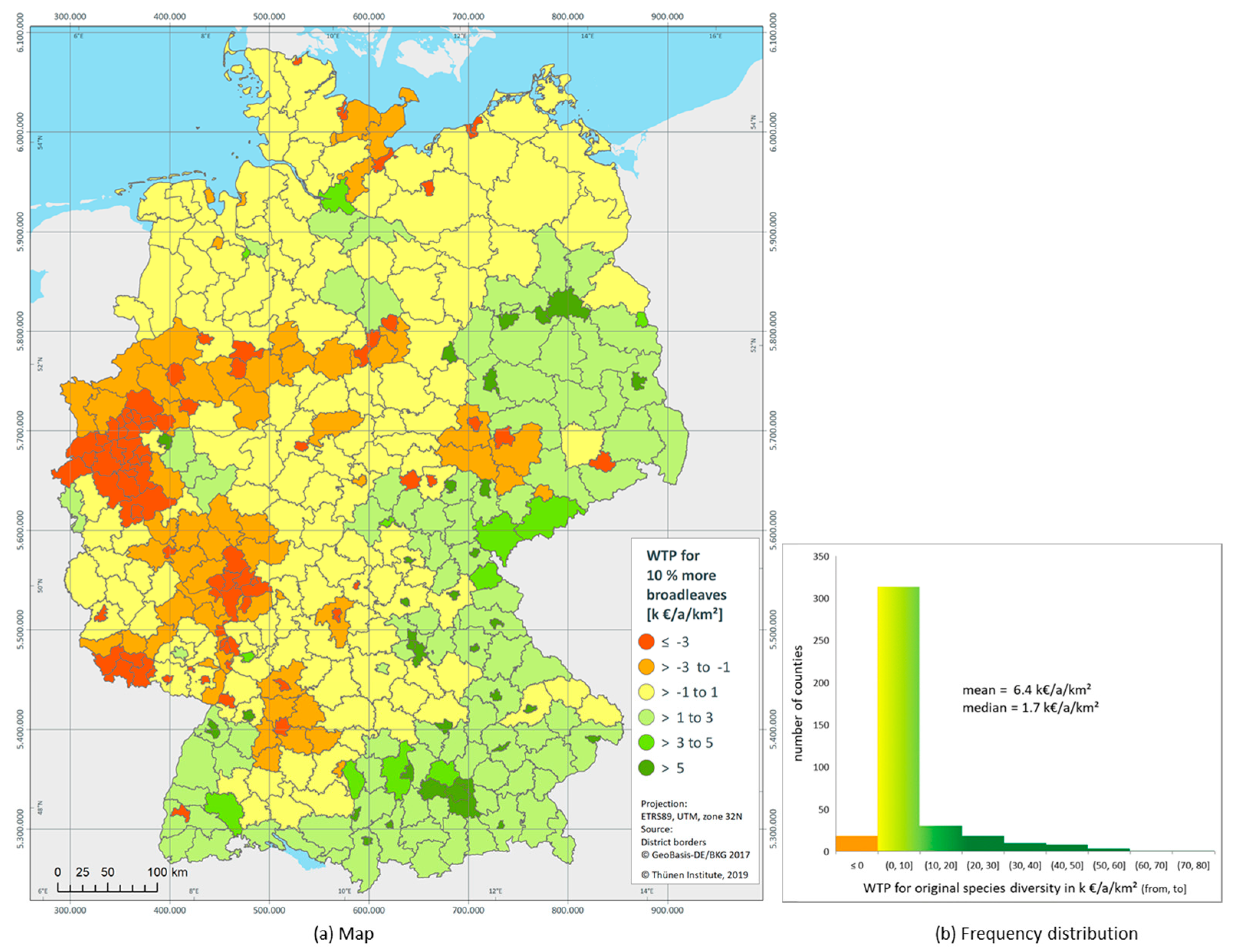
3.4. Annual Benefits of Increased Forest Biodiversity

As argued above, it is not meaningful to calculate an overall value of forest biodiversity protection services in the status quo (because the status quo includes essential parts that are not substitutable). What is possible and relevant, instead, is the valuation of marginal changes of this status quo. The goal of reversing past biodiversity losses and restoring natural diversity, which explicitly or implicitly inspires several federal government strategies [53,107,108], is used here to determine the benefits of increased forest biodiversity. We apply a scenario in which the (hypothetical) original species diversity in forests is assumed to be restored everywhere in Germany. This is done by setting the sub-index forests of the indicator “Species Diversity and Landscape Quality” to the target value of 100 in all counties. By design, this target value implies a complete restoration of species diversity in the forests as it may have existed in a presumed past. The current value of the sub-index fluctuates around 85, with values between 79.2 and 90.1 since 2010 [52]. Hence, the scenario corresponds to an average increase in species diversity of 15 percentage points.

Summing up the benefits across all counties, achieving the restoration target would result in benefits of 899 million €/a (alternatively assuming a current index value of 80 points, the increase would be 20 rather than 15 index points and the WTP would amount to 1186 million €/a; with a current index value of 90 points, it would be 611 million €/a). Checking the result against a comparable study at the national level, which elicited the WTP for an increase by 20 index points [121], our estimate is about 9% lower, with confidence intervals that mutually include the means (indicating that there is no statistically significant difference between the two estimates at the 5% level).

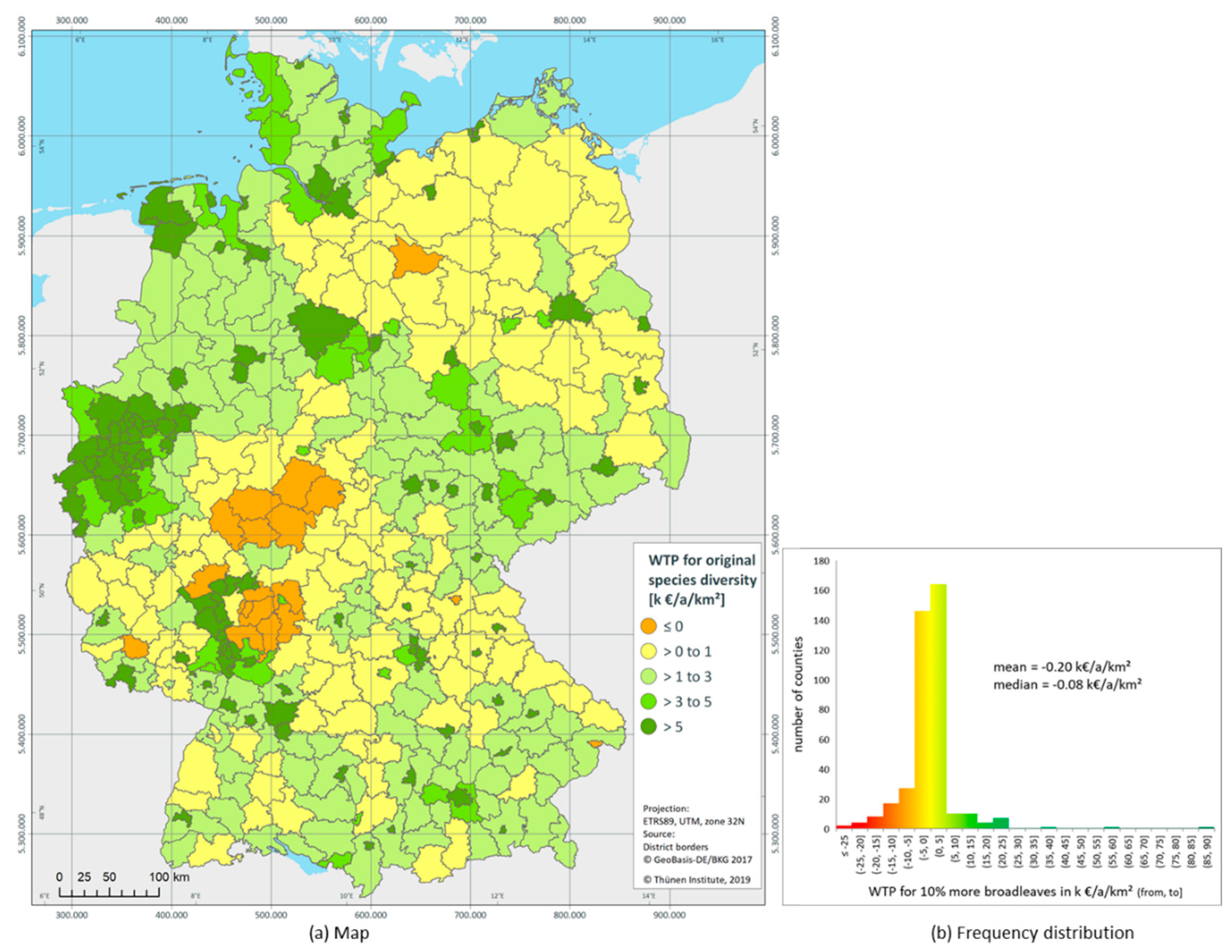
Looking at the spatial distribution (Figure 8), the first thing to notice are a few areas where the model calculates a negative benefit (marked in red). These are regions in which the sub-index forests already exceeds 100 index points today; a target value of 100 thus arithmetically implies a biodiversity loss (which of course would not be pursued as a political goal). In most other counties, the aggregated WTP for an increase in forest biodiversity is between 0 and 10 k€/a/km².However, there are areas with much higher benefits (up to 77 k€/a/km²). Such areas are found everywhere where forest biodiversity is low today (so that there is much to improve) and/or the population density is high (so that many people would benefit from such improvements). This is typically the case in regions characterized by industry or intensive agriculture, many of which are located in the west and north-west of the country.

3.5. Annual Benefits of Increasing the Share of Deciduous Trees

A widespread concern among nature conservationists and foresters is to reduce the formerly anthropogenically increased proportion of conifers in favor of deciduous trees. The goal of converting (coniferous) pure stands into site-adapted deciduous and mixed forests has also found its way into the National Biodiversity Strategy [107] and the Forest Strategy 2020 [108]. Within the framework of the “European Beech Initiative” [122], nature conservationists are particularly interested in the beech, which was originally typical of the German landscape and now covers only about one sixth of the forest area [123]. In order to examine the effects of a (moderate) increase in the proportion of deciduous trees—and in particular, the proportion of beech—we calculate a scenario in which the proportion of beech in the forest area is increased by 10 percentage points in each county. Correspondingly, the conifer area is reduced (with a proportional reduction of the individual conifer species). Since the aforementioned political demands are not underpinned by concrete target values for the proportion of deciduous trees or beech, the simulated increase is based on the computationally optimal proportion from a landscape preferences point of view (see Table 5, results for all respondents); it is about 10 percentage points higher than today.

Accumulated, the benefit from the altered landscape scenery amounts to about 130 million €/a on balance. However, there are both gains and losses (see Figure 9), following a striking geographical gradient. Counties recording gains are mainly located in the eastern and southern parts of the country and are rich in coniferous forests. However, this is offset by losses in other areas that are already rich in deciduous trees: In these counties a further increase in the proportion of deciduous trees would worsen the landscape scenery for the population; negative values are to be interpreted here as willingness to pay for a (moderate) increase in the proportion of conifers. This is especially the case in the western part and along the Baltic Sea coast. In the remaining area, gains and/or losses are comparatively smaller. The frequency distribution shows that for 77% of the counties, these changes fall within the range between −5 and +5 k€/a/km². Losses, however, can be up to −29 k€/a/km² in the extreme, gains even up to +87 k€/a/km². The mean value across counties is very close to zero (but note again that this is a mean of counties with normalized area, not a population mean).

4. Discussion

In this article we investigated the economic benefits of fundamental forest ecosystem services for the population in Germany at national level and estimated the spatial distribution of these benefits. Overall, the annual benefits in the current status quo as well as in the example scenarios demonstrate that the German society profits considerably from the ecosystem services of its forests—far beyond what is reflected in the market statistics. At the same time, the spatial distribution of the services reveals pronounced differences: While services for timber production and climate protection are most prominent in the low mountain ranges and the sparsely populated, densely wooded regions of the lowlands, recreational services dominate around urban centers. The scenario analyses reveal that the potential to increase benefits by restoring the original forest biodiversity is particularly high in the less forested parts of the northern half of the country, and again in many cities, where a high number of people benefit from such improvements. The benefits of increasing the share of deciduous trees, on the other hand, follow a geographical gradient, with gains distributed predominantly across the southern and eastern parts, while losses are concentrated in parts of the west and in the far north.

There are a number of caveats that need to be considered when interpreting our model results. First of all, the limited quality of many of our input data should be kept in mind. Some are not fully representative in a statistical sense (e.g., the timber prices from the forest accountancy network), others are subject to a high sampling error (e.g., the data from the forest growth areas that subsequently have been assigned to the municipality level), and still others rely on stated preference valuation approaches with their typical problems [124,125,126], or more generally on self-reporting of respondents rather than independently verifiable observation (e.g., population survey data). Likewise, there is no single reference date; rather, the original input data have been collected at different points in time between 2012 and 2018 [(forest growth and harvest data even go back to the decade between the last two forest inventories in 2002 and 2012, respectively)]. Accordingly, the data approximately describe the past decade as a whole. As a consequence, the model does not provide “exact” benefit estimates, and certainly not for individual counties. Rather, it should be understood as a large-scale model that primarily intends to uncover regional patterns of service values.

As to comparisons between the individual services, an important point is that the benefit estimates are each based on different valuation approaches. In particular, the valuation of timber production differs conceptually from that of the other (public) services, as it rests on prices instead of surplus measures. However, even if, in an alternative interpretation, both can be considered as measures of income effects at the macroeconomic level [127], methodological differences remain that limit the comparability between the individual services. In particular, the contingent valuation approach with open ended questions used in this study for valuing recreation tends to produce lower value estimates than the discrete choice experiments applied for valuing conservation services [102,128], even if both attempt to ensure consequentiality. For example, studies that elicited the right of access to specific areas by means of choice experiments arrived at recreation values that were 2 to 3 times higher than comparable contingent valuation studies [129,130]. In the case of climate protection, there are not only many uncertainties in the valuation [94], but even in the quantification of the physical basis. These uncertainties compel applying generalized assumptions (e.g., with regard to substitution factors), as well as neglecting individual storage compartments in a situation where no reliable predictions can be made about their development (in the present case, this concerns, e.g., the neglect of underground biomass and soil carbon). The value relations between the individual services should therefore be interpreted with caution; the model provides more reliable information about the spatial distribution pattern of a particular service (and its simulated changes) than about the value relations of different services.

When interpreting these patterns, it is important to remember that our spatial valuations are generally based at average preferences of the German population, and estimated benefit differences are mostly due to differences in the underlying physical quantities (for example, differences in aggregate biodiversity benefits are due to different values of the diversity indicator in each county, but they use the same mean WTP estimate for Berliners as for Bavarians). An exception is the valuation of the ratio of deciduous trees to conifers, in which the model takes the local tree species composition into account. Further possible preference differences across regions could not be captured, as this would usually require a much larger and more detailed pool of input data.

Finally, it needs some discussion how the model deals with aspects of time and tree age—a standard problem of forest economics. Static models, such as the present one, do not capture the dynamic aspects of forest growth; what is possible, however, is a comparison of scenarios in which given forest stands are hypothetically replaced by alternatively composed stands. Scenarios that aim at changes in forest composition (e.g., through afforestation or changes in tree species composition) can therefore only be interpreted in terms of their long-term effects, or alternatively as “what-if” analyses (e.g., “What if a region was not dominated by the given conifers, but by deciduous trees of the same age?”). An interpretation in terms of long-term effects necessarily requires the assumption that population preferences remain stable over time.

What are the options for further development? For one, it seems worthwhile to close obvious gaps with regard to further forest ecosystem services that have not yet been included in the model (like, e.g., water provisioning services), as well as to integrate other land use forms that provide some of the same ecosystem services as forests, but also additional ones (especially agricultural ecosystems). Suitable candidates and cold/hot spots of ecosystem provision have already been identified in the literature [131,132]. For another, an update of the data would be desirable, in particular because two recent events are likely to have changed the value relations between forest ecosystem services to some extent: the drought and bark beetle damages of the last three years in large parts of Central Europe [133,134,135], which have both changed the composition of the forests and impaired timber prices; and the lockdowns due to the Coronavirus pandemic, which may have made many people reassess the values of forests as places of retreat [136,137,138,139].

5. Conclusions

Notwithstanding the caveats mentioned above, our results demonstrate that a spatially explicit valuation for an entire country is possible even if local case studies are not available in abundance. We provide for the first time such a spatial valuation for some important forest ecosystem services in Germany. The methodology we have developed, which is predominantly a benefit transfer approach utilizing regression sampling methods, might be useful for other countries with a similar background situation. Thus, it could help overcome the widespread lack of regionally differentiated data, especially for the protection and management of those forest ecosystem services for which markets do not exist.

In practical terms, recognizing the spatial patterns of ecosystem benefits can help policy makers to improve the institutional setting for protecting and developing forests beyond centrally standardized blanket targets, i.e., to allocate changes in forest management where this will have the highest benefit (for a concrete concept under German conditions, see e.g., [140]). This can contribute to protecting and using forest resources and forest ecosystem services more sustainably and efficiently—for the benefit of people as well as nature.