CNN-Based Individual Tree Species Classification Using High-Resolution Satellite Imagery and Airborne LiDAR Data

Abstract

Deep learning (DL) has shown promising performances in various remote sensing applications as a powerful tool. To explore the great potential of DL in improving the accuracy of individual tree species (ITS) classification, four convolutional neural network models (ResNet-18, ResNet-34, ResNet-50, and DenseNet-40) were employed to classify four tree species using the combined high-resolution satellite imagery and airborne LiDAR data. A total of 1503 samples of four tree species, including maple, pine, locust, and spruce, were used in the experiments. When both WorldView-2 and airborne LiDAR data were used, the overall accuracies (OA) obtained by ResNet-18, ResNet-34, ResNet-50, and DenseNet-40 were 90.9%, 89.1%, 89.1%, and 86.9%, respectively. The OA of ResNet-18 was increased by 4.0% and 1.8% compared with random forest (86.7%) and support vector machine (89.1%), respectively. The experimental results demonstrated that the size of input images impacted on the classification accuracy of ResNet-18. It is suggested that the input size of ResNet models can be determined according to the maximum size of all tree crown sample images. The use of LiDAR intensity image was helpful in improving the accuracies of ITS classification and atmospheric correction is unnecessary when both pansharpened WorldView-2 images and airborne LiDAR data were used.

1. Introduction

Trees can reduce urban air pollution and noise, prevent soil erosion, and beautify the environment, which is important for ecosystems. The identification and mapping of the composition of tree species and the analysis of spatial distribution of tree species is crucial for forest conservation and urban planning and management. The remote sensing technology, which has the advantages of covering large areas and revisiting after several hours or days, has been employed in tree species identification for decades [1,2]. As early as the 1960s, aerial photographs were explored for the recognition of tree species [1]. In 1980, Walsh explored satellite data (such as Landsat) to identify and map 12 land-cover types, including seven coniferous forest types [2]. Early studies on tree species classification were mainly conducted at the pixel level [3,4]. For example, Dymond et al. used multitemporal Landsat TM imagery to improve the classification accuracy of deciduous forests at the landscape scale [3]. Tree species classification at individual tree level using high-resolution imagery can also date back to the 2000s [5,6,7]. The related works were mainly conducted using high-resolution aerial photographs. The rapid development of platforms and sensors makes the availability of high-resolution multisource data, such as airborne hyperspectral imagery and airborne LiDAR data. Recently, a large number of works at individual tree level explored the use of airborne hyperspectral and LiDAR (light detection and ranging) data, or the combination of the two [8]. Studies showed that the individual tree species (ITS) classification using the combined airborne hyperspectral images and airborne LiDAR data obtained higher accuracy than a single data source [9,10,11,12,13]. For example, hyperspectral and LiDAR data were fused at pixel-level by Jones et al. [9] and then employed to classify 11 tree species in temperate forests of coastal southwestern Canada. The classification using a support vector machine (SVM) achieved an overall accuracy (OA) of 73.5%. Furthermore, individual tree crown-based classification has been demonstrated to perform better than pixel-based classification. Alonzo et al. [10] used the fusion of airborne visible/infrared imaging spectrometer (AVIRIS) imagery and airborne LiDAR data to map 29 common tree species at tree crown level in an urban area of the USA, which yielded an OA of 83.4% using canonical discriminant analysis. Shen and Cao [11] employed random forest (RF) to classify individual tree crowns using airborne hyperspectral and LiDAR data covering a subtropical forest in southeast China. An OA of 90.6% was achieved by the classification using both hyperspectral and LiDAR metrics, considering only sunlit portions of tree crowns. The outstanding performances of such works mainly attribute to the useful spectral and textural characteristics provided by airborne hyperspectral imagery, along with heights and structural metrics derived from airborne LiDAR data [9].

The recent increase in the availability of high spatial resolution satellite imagery, such as WorldView-2/3/4, has attracted a lot of attention to exploiting its use in ITS classification [14,15,16,17,18,19]. For example, Pu et al. [14] evaluated the capabilities of IKONOS and WorldView-2 (WV-2) to identify and map tree species of urban forest. Their results demonstrated the potential of WV-2 imagery for the identification of seven tree species in urban area. The classification using a decision tree classifier (CART) achieved an OA of 62.93%. Madonsela et al. [17] used multi-phenology WV-2 imagery and RF to classify savannah tree species. An OA of 76.40% for four tree species was achieved. The combination of high-resolution aerial or satellite images and airborne LiDAR data has also been explored for ITS classification [20,21,22,23]. Specifically, Deng et al. [20] compared several classification algorithms for the classification of four tree species using simultaneously acquired airborne LiDAR data and true colour (RGB) images with a spatial resolution of 25 cm. Several classification algorithms were employed, and the highest OA (90.8%) was provided by the quadratic SVM.

Based on the literature, exemplified by the above-mentioned studies, the most commonly used classifiers for ITS classification are SVM and RF. One of the challenges for this kind of classification algorithms is the extraction and selection of useful features that are crucial for accuracy. As a result, deep learning (DL) is gaining attention in ITS classification due to its capability of automatic learning from examples and allowing features to be extracted directly from data. DL, inspired by the human visual perception system, has initially gained success in computer vision and medical applications. Typical DL networks include convolutional neural networks (CNNs), stacked autoencoders, deep belief networks, and recurrent neural networks. Among these networks, CNNs are the most potential and popular for perceptual tasks. The application of CNNs has grown very fast in remote sensing since 2014. CNNs have been successfully used in various remote sensing tasks, such as image scene classification, object detection, image pan-sharpening and super-resolution, image registration, and image segmentation [24,25,26,27]. In the context of remote sensing image classification, the commonly used CNN models include AlexNet [28], VGG [29], ResNet [30], Dense Convolutional Network (DenseNet) [31,32]. Despite the popularity of CNN in remote sensing image classification, its exploration in ITS classification is still limited. In 2019, Hartling et al. [33] examined the potential of DenseNet in the identification of dominant tree species in a complex urban environment using the combination of WV-2 VNIR, WV-3 SWIR, and LiDAR datasets. DenseNet-40 yielded an OA of 82.6% for the classification of eight dominant tree species, which was significantly higher than those obtained by RF and SVM.

In this study, a comprehensive analysis of several CNN models (ResNet-18, ResNet34, ResNet-50, and DenseNet-40) for ITS classification was performed using the combination of the panchromatic band of WV-2, a pansharpened version of the WV-2 multispectral imagery, and a digital surface model (DSM) and an intensity map derived from airborne LiDAR data. The performances of the CNN models were also compared with those of traditional machine learning classification methods (such as RF and SVM). The helpfulness of the LiDAR intensity map and the atmospheric correction of the WV-2 imagery were analyzed to provide detailed directions for related studies. The input size of sample images of ResNet and DenseNet was firstly discussed in this work, which is meaningful for improving the performances of CNN models in ITS classification.

2. Study Area and Data

2.1. Study Area

The study area of this work is located on the Keele campus of York University, Toronto, Canada (centered at 43.7735° N, 79.5019° W), as shown in Figure 1a. Trees mainly grow along roads and in wood lots. The primary tree species in this area include maple, ash, locust, oak, pine, and spruce.

2.2. Datasets

The WorldView-2 (WV-2) imagery, acquired in July 2016, was provided by the York University Map Library. The WV-2 image includes one panchromatic (PAN) band and eight multispectral (MS) bands. The spatial resolution of the PAN band and MS bands is 0.4 m by 0.4 m and 1.6 m by 1.6 m, respectively.

The LiDAR data was collected using a Leica ALS70 system in April 2015 at a flying height of 1300 m and a flying speed of 160 knots (82.3 m/s). The data has an average point density of approximately 10.0 pts/m². The LiDAR elevations were compared with independently surveyed ground points to quantify the accuracy statistically. The horizontal accuracy was 30 cm, whereas the fundamental vertical accuracy was 10 cm.

An inventory map of the study area was provided by the campus services and business operations of York University. The inventory map recorded more than 5000 trees with their attributes, including species, heights, crown sizes, and diameter breast height. The initial survey of the trees was carried out in 2014, and the measurements were then updated in 2015.

3. Methodology

Four object-based CNN networks were designed and implemented in this study to classify four tree species using the combined WV-2 imagery and LiDAR data. The flowchart of the method is presented in Figure 2 [34].

The LiDAR point cloud was first processed using ENVI LiDAR Version 5.3.0 (L3Harris Geospatial, Broomfield, CO, USA) to generate a digital surface model (DSM), a digital elevation model (DEM), and an intensity image. The intensity of LiDAR data was defined as the amount of reflected energy at the peak amplitude of the returned signal and has been demonstrated to be useful for distinguishing different tree species [35,36]. ENVI LiDAR filtered the point cloud data with filters based on triangulated irregular network (TIN) for the generation of DEM. We used the default parameters provided by the software, which include the maximum error of terrain TIN of 10 cm and the maximum TIN polygon density of 10,000. The intensity image and the DSM were produced with a spatial resolution of 0.25 m. The DEM was generated with a spatial resolution of 0.5 m, the highest resolution for DEM provided by the software. The DSM, DEM, and intensity image were then resampled to the spatial resolution of 0.4 m by 0.4 m using MATLAB to match the spatial resolution of the WV-2 imagery. A normalized DSM (nDSM), which is also referred to as a canopy height model (CHM), was derived as the difference between the DSM and DEM using MATLAB. Atmospheric correction was performed on the MS bands of the WV-2 imagery using the FLAASH Atmospheric Correction Model of the ENVI software to obtain an 8-band reflectance image of the study area. The resulting reflectance image was then orthorectified base on the DSM and the LiDAR intensity, along with the PAN band. Then, a pansharpened MS image with a spatial resolution of 0.4 m was produced through the fusion of the PAN band with the 8-band reflectance image. The fused MS, PAN, and the nDSM were then used to delineate individual tree crowns. Regarding the tree crowns and the inventory map, tree species samples were manually selected and labeled to obtain the sample dataset. Finally, three ResNet models and a DenseNet model were used to classify the tree species, and the classification results were evaluated and compared with traditional machine learning classification methods, namely SVM and RF. The four CNN models were selected because they gave excellent performances in similar works. The details of the four CNN models can be found in Section 3.4.1.

The details of image orthorectification, individual tree crown delineation, tree crown sample generation and sample dataset preparation, tree species classification using CNN models and traditional machine learning methods, and accuracy assessment metrics are introduced in the following subsections.

3.1. Image Orthorectification

The orthorectification of the MS and PAN bands of WV-2 imagery was carried out by using the ENVI software (L3Harris Geospatial, Broomfield, CO, USA). Eight GCPs that were manually identified across the whole image were employed in the orthorectification to align the MS and PAN images with the LiDAR data. A sub-pixel accuracy (with the root mean square error of 0.43 pixel) was achieved. The orthorectified PAN image is shown in Figure 3 as an example.

The orthorectified PAN and MS images were then fused using the Gramm-Schmidt pansharpening method provided in the ENVI software. The resulting pansharpened MS image with a spatial resolution of 0.4 m and the LiDAR nDSM were then employed for the delineation of individual tree crowns.

3.2. Individual Tree Crown Delineation

Both the pansharpened MS image and the LiDAR nDSM were used for the individual tree crown delineation. To separate trees from buildings and grasses, a hierarchical rule-based classification method proposed in [37] was first employed to produce a classification map with six categories, including building, road, tree, grass, water body, and shadow. During the classification, ground pixels were first separated from the non-ground pixels based on the height information provided by the nDSM map. The non-ground pixels were then divided into the tree class and the building class based on the corresponding values in a normalized difference vegetation index (NDVI) map generated using the pansharpened MS image. A preliminary tree map was then obtained based on the tree class. In this work, the NDVI was generated using the red and NIR1 bands of the WV-2 imagery. A subset of the pansharpened MS image and nDSM is shown in Figure 4a,b, respectively. A subset of the tree map is shown in Figure 4c. Due to the difference in acquisition time and the residual of co-registration, the preliminary tree map may include some pixels that are not corresponding to trees in the nDSM map. To obtain tree crowns that match well with both the WV-2 images and nDSM, only the overlapped portion of the preliminary tree map and nDSM were used for individual tree crown delineation. Therefore, the pixels that have high values in nDSM but do not belong to tree pixels in the preliminary tree map were set to zero. This resulted in a modified version of the nDSM map, which was used in the following steps for individual tree crown delineation.

The multiscale analysis and segmentation (MSAS) method proposed in [38] was used for the delineation of individual tree crowns from the nDSM map. The MSAS method consists of three steps. The first step involved scale analysis to determine the sizes of multiscale morphological filters, which were used to detect tops of tree crowns of different sizes. Next, the nDSM map was filtered at multiple scale levels, and the marker-controlled watershed segmentation method was then adopted to detect candidate tree crowns of different sizes. Finally, the candidate tree crowns were merged to produce a tree crown map. In this work, scale sizes ranging from 9 to 23 pixels with a step of 2 pixels were used in the first step. The resulting tree crown map was manually refined according to the LiDAR data to eliminate some false positives, which were mainly caused by the different acquisition times of the WV-2 imagery and LiDAR. For example, some ashes shown in the LiDAR data disappeared in the WV-2 imagery. A subset of the individual tree crown map is shown in Figure 4d. The refined version was finally converted to tree crown polygons to facilitate the selection of tree crown samples.

3.3. Tree Crown Sample Generation and Sample Dataset Preparation

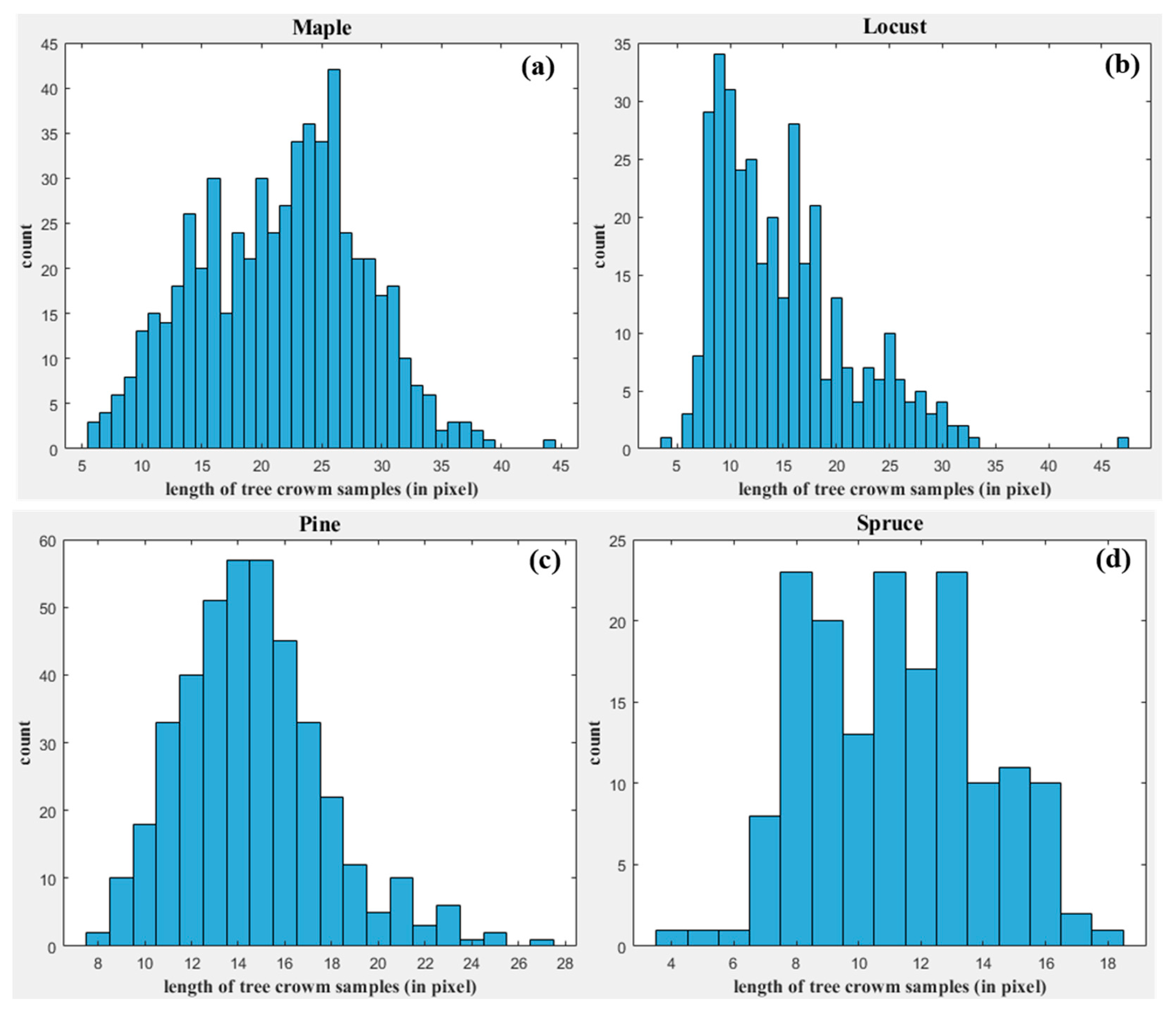
Tree samples were manually selected from the delineated tree crown polygons, as shown in Figure 4e,f. Some of the tree crown polygons were further validated using a field investigation. Finally, as shown in

Table 1. The statistics of the sample dataset.

Tree Species	Sample Set			Training Sample Set after Data Augmentation
	Total	Testing	Training
Maple	580	174	406	2436
Locust	351	105	246	1476
Pine	408	123	285	1710
Spruce	164	49	115	690
Total	1503	451	1052	6312

, we obtained 1503 samples in total, which include 580, 408, 351, and 164 samples for maple, pine, locust, and spruce, respectively.

The tree crown sample images with 11 bands were generated through using two steps. First, the PAN band, eight fused MS bands, intensity image, and nDSM were merged band by band to produce a single image with 11 bands. This image was then clipped according to the minimum exterior rectangle of each tree crown polygon to produce tree crown sample images with a band number of 11.

The tree crown sample images were divided into two parts, which were used for training and testing, respectively. For each species, 70% (1052 in total) of the sample images were used for training, while the other 30% (451 in total) were used for testing.

We adopted data augmentation to increase the number of training samples. Specifically, the original sample images were rotated by 90°, 180°, and 270°, separately and flipped horizontally and vertically. A total number of 6312 training samples were obtained, as presented in Table 1.

3.4. Tree Species Classification

3.4.1. CNN Models

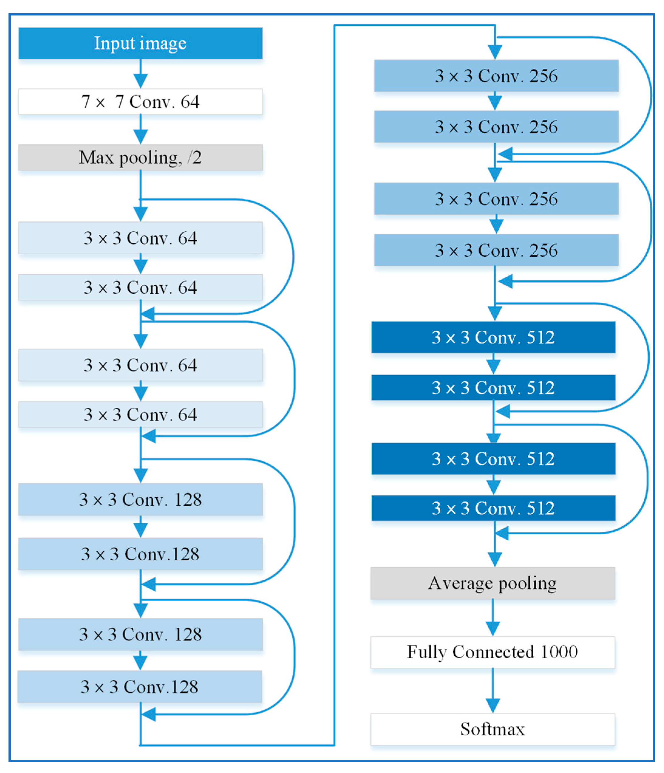
Typical CNN models include convolutional layers, pooling layers, and fully connected layers. The residual learning framework was proposed to resolve the degradation problem exposed during the training of deep networks [30]. Residual networks were implemented by inserting shortcut connections into plain networks, which add no extra parameters or computational complexity. Several ResNet models with different numbers of layers, which include ResNet-18, ResNet-34, ResNet-50, ResNet-101, and ResNet-105, were proposed. Compared with the sizes of sample images used for scene classification, the size of tree crown samples was relatively small. Deeper networks have more convolution layers and more pooling layers which are used to reduce the size of output features. When the size of output features was reduced to 1 × 1 after a pooling layer, no additional features can be extracted by the following layers. In this case, some parameters may be untrainable. Deeper networks may even provide lower classification accuracy if the input image have relatively small sizes. Consequently, ResNet models with a relatively shallow network, such as ResNet-18, ResNet-34, and ResNet-50, were used in this work for ITS classification. As an example, the architecture of ResNet-18 is shown in Figure 5. It comprises a convolutional layer with a filter size of 7 × 7, 16 convolutional layers with a filter size of 3 × 3, and a fully connected layer. A shortcut connection is added to each pair of 3 × 3 filters, which constructs a residual function.

Inspired by the idea of adding shortcut connections, DenseNet was proposed in 2017 [31]. It is approved that DenseNets have some advantages, such as alleviating the problem of vanishing-gradient and strengthening the propagation of feature. They can also reduce the number of parameters. DenseNets include multiple densely connected dense blocks and transition layers. Transition layers are the layers between dense blocks. Each transition layer consists of a 1 × 1 convolutional layer followed by a 2 × 2 average pooling layer. A similar reason for the use of ResNet models, DenseNet-40, which has a shallower architecture than other DenseNets, was employed in this study. DenseNet-40 has three transition layers and three dense blocks, which have a growth rate of 4. Figure 6 shows its architecture.

Compared with traditional machine learning methods, the advantage of CNN-based classification methods is that we do not need to design and select features used for classification. Instead, we just need to feed sample images (of which the bands we can design) into the models. Three experiments using different band combinations were performed for the classification using the CNN models. As shown in

Table 2. The band combinations used for the classification using CNN models.

Name	Bands	Total Number
P	The PAN band	1
P+M	The PAN and eight pansharpened MS bands	9
P+M+H	The PAN and eight pansharpened MS bands and the nDSM	10
P+M+H+I	The PAN and eight pansharpened MS bands, the nDSM and the the intensity image	11

, the first combination used only the PAN, denoted as P, and the second band combination used both the PAN and eight pansharpened MS bands, denoted as P+M. The third considered both the WV-2 imagery and LiDAR nDSM map was denoted as P+M+H, whereas the forth combination including the WV-2 imagery and the LiDAR nDSM and the intensity image was denoted as P+M+H+I.

For CNN-based ITS classification, all the training and testing samples were resized to a size of 32 × 32 pixels, according to the average size of all the tree crown samples. The classification using the four CNN models was performed on Python 3.6 and Keras 2.2. The Adam optimizer was employed. The initial learning rate and the maximum epoch number were set to 0.001 and 500, respectively. An early stopping strategy was also employed to avoid over-fitting problems.

3.4.2. Traditional Machine Learning Classification Methods

As commonly used traditional machine learning classification methods for land cover classification, RF and SVM algorithms were considered in this work for ITS classification. As introduced in Section 3.4.1, we need to select useful features for the two classifiers. This is different from CNN-based classification, which has the capability of automatic learning from examples and allowing features to be extracted directly from images. As shown in

Table 3. Feature variables used for traditional machine learning classification.

Feature Name	Description	Image Bands	Feature Number
SpecMean	Mean value of each sample in each spectral band	PAN+MS	9
SpecStd	Standard deviation of each sample in each spectral band		9
TextCon	Contrast of the GLCM texture of each sample	PAN	4
TextCor	Correlation of the GLCM texture of each sample
TextEn	Energy of the GLCM texture of each sample
TextHom	Homogeneity of the GLCM texture of each sample
H_Max	Maximum height of each sample	nDSM	10
H_Min	Minimum height of each sample
H_Mean	Mean height of each sample
H_Std	Height deviation of each sample
Area/H_Max	Ratio of crown area to the maximum height of each sample
Area×H_Max	Product of crown area and the maximum height of each sample
H_Max-H_Mean	Difference between the maximum crown height and the mean height of tree crown
(H_Max-H_Min)/H_Max	Ratio of the difference between the maximum and minimum of crown heights to the maximum crown height
(H_Max-H_Mean)/H_Max	Ratio of the difference between the maximum and mean of crown heights to the maximum crown height
H_Std/H_Max	Ratio of standard deviation of tree crown heights to the maximum crown height
		Total	32

, spectral and texture features from the WV-2 imagery and height metrics derived from nDSM were calculated for each tree crown sample [12]. A number of 18 spectral features were obtained using the mean and standard deviation of the PAN and pansharpened MS bands. Texture features were extracted from the PAN band using the grey-level co-occurrence matrix (GLCM). The considered texture metrics include contrast, correlation, energy, and homogeneity [22,39,40]. In this case, 10 height variables, as shown in Table 3, were extracted from the nDSM [13,20,23,41].

Additionally, five vegetation indexes were considered for both the RF and SVM. The indexes include the normalized difference vegetation index (NDVI) [42,43,44] using NIR1, the NDVI using NIR2 [45], the green normalized difference vegetation index (GNDVI) [45,46], the enhanced vegetation index (EVI) [46,47], and the visible atmospherically resistant indices (VARI) [48,49] using the red-edge band. The details of the five indexes are shown in

Table 4. Vegetation indexes employed for ITS classification.

Vegetation Index Name	Abbreviation	Formula	References
Normalized Difference Vegetation Index	NDVI	(NIR1 − RED)/(NIR1 + RED)	[43,44,45]
Normalized Difference Vegetation Index-NIR2	NDVI2	(NIR2 − RED)/(NIR2 + RED)	[46]
Green Normalized Difference Vegetation Index	GNDVI	(NIR1 − GREEN)/(NIR1 + GREEN)	[46,47]
Enhanced Vegetation Index	EVI	2.5 × (NIR1 − RED)/(NIR1 + 6 × RED − 7.5 × BLUE + 1)	[47,48]
Visible Atmospherically Resistant Index	NDVI-RE	(RED_EDGE − RED)/(RED_EDGE + RED)	[48,49]

.

Different feature combinations were tested for the classification using RF and SVM. As shown in

Table 5. Feature combinations considered for the RF and SVM classifiers.

Name	Features	Number
P	SpecMean and SpecStd of the PAN band	2
P+M	SpecMean and SpecStd of the PAN and pansharpened MS bands	18
P+M+V	SpecMean and SpecStd of the PAN and pansharpened MS bands and five vegetation indices	23
P+M+V+T	SpecMean and SpecStd of the PAN and pansharpened MS bands, five vegetation indices, and four GLCM texture features	27
P+M+V+T+H	SpecMean and SpecStd of the PAN and pansharpened MS bands, five vegetation indices, four GLCM texture features, and 10 height variables derived from the nDSM	37
P+M+V+T+H+I	SpecMean and SpecStd of the PAN and pansharpened MS bands, five vegetation indices, four GLCM texture features, 10 height variables derived from the nDSM, and the mean and standard deviation of the LiDAR intensity image	39

, six feature combinations were considered in the experiment. The first four feature combinations considered only the WV-2 imagery, while the other two combinations involved both the WV-2 imagery and airborne LiDAR data. The feature combination P+M+V+T+H+I was compared with the feature combination P+M+V+T+H to evaluate the effectiveness of the LiDAR intensity image for tree species classification. We used the radial basis function as the kernel function for the SVM classifier and a decision tree parameter of 500 for the RF classifier.

3.5. Accuracy Assessment

A confusion matrix was employed to evaluate the accuracy of ITS classification using the testing samples. Producer accuracy (PA), user accuracy (UA), OA, and kappa coefficient were derived from the matrix. Average accuracy (AA) was the average of PA and UA.

4. Experimental Results

4.1. Results of the CNN Models

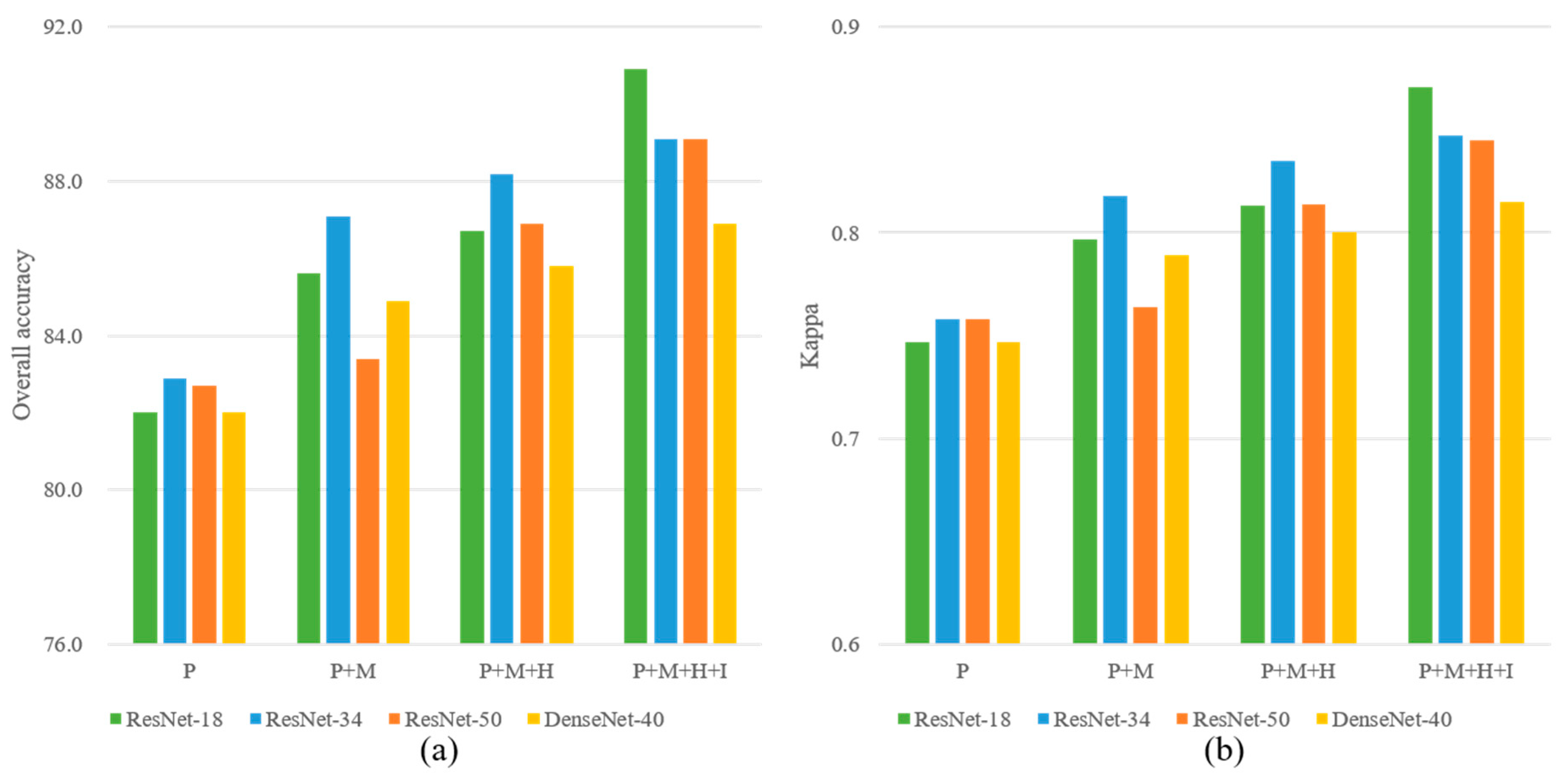
The OA and kappa values of CNN-based classification using the four band combinations P, P+M, P+M+H, and P+M+H+I are shown in Figure 7, and the AA values of each tree species are presented in Figure 8. It can be observed that the band combination P+M+H+I provided the highest OAs for each CNN model, followed by the band combinations P+M+H and P+M. This finding supports the importance of the nDSM and intensity image in improving the classification accuracy. For example, the OA of ResNet-18 obtained using the band combination P+M+H+I was 90.9%, which was increased by 5.3% compared with that of the band combination P+M. The AA values of Locust, Pine, and Spruce were also increased by 5.4%, 8.6%, and 15.6%, respectively. The band combination P+M yielded higher OAs than those of the band combination P using only the WV-2 PAN imagery, indicating the effectiveness of the eight MS bands for ITS classification.

Among the four CNN models, ResNet-18 and ResNet-34 yielded higher OA values than the other two CNN models for the band combinations P+M, P+M+H, and P+M+H+I. ResNet-18 provided the highest OA values for the band combination P+M+H+I, whereas ResNet-34 offered the highest OA values for the band combination P+M and the band combination P+M+H.

In terms of the AA accuracies of each tree species, the highest AA values of the four tree species were reached by ResNet-18 using the band combination P+M+H+I. The AA values of the pine class were the highest, followed by those of the maple and spruce class. In contrast, the AA values of the locust class were the lowest. For the spruce class, the band combination P+M+H+I offered significantly higher AA values than those of the combinations P+M and P+M+H, indicating that LiDAR intensity data is crucial for improving the classification accuracy of spruce.

4.2. Results of the RF and SVM

The corresponding classification results are presented in Figure 9 and Figure 10. It shows that SVM achieved higher OA and kappa coefficients than RF for each of the six feature combinations. The feature combination P+M+V+T+H+I yielded the highest OA values, whereas the feature combination P obtained the lowest OA values for both RF and SVM. The OA values of the feature combination P+M+V using RF and SVM were not higher than those of P+M, indicating that the inclusion of the five vegetation indices provided limited improvements in the accuracy. In contrast, P+M+V+T yielded significantly higher OA values than P+M. This result indicated that it was very necessary to include texture features when only on the WV-2 imagery was considered for ITS classification. The feature combination P+M+V+T+H improved the accuracy more significantly than P+M+V+T, indicating the importance of LiDAR nDSM in the classification. The feature combination P+M+V+T+H+I yielded higher OA values than those of P+M+V+T+H for both RF and SVM. This indicates that the consideration of the LiDAR intensity image is also helpful for improving the classification accuracy.

Additionally, SVM offered higher AA values for all four tree species than RF for the feature combinations P+M+V+T and P+M+V+T+H+I. For SVM, the AA value of the pine class was higher than other classes, while that of the locust class was the lowest. Similar results can also be observed for RF.

4.3. Comparisons between CNN Models and Machine Learning Methods

Comparisons between CNN models and machine learning methods were conducted in two aspects in this study. First, the ITS classification accuracies of CNN models and traditional machine learning obtained using only the WV-2 imagery were compared. As shown in

Table 6. Classification accuracies of the four CNN models, RF, and SVM obtained using only the WV-2 imagery. The accuracies of four CNN models were yielded using the band combination P+M and those of RF and SVM were obtained using the feature combination P+M+V+T.

Model	Class	PA (%)	UA (%)	AA (%)	OA (%)	Kappa
ResNet-18	Maple	90.4	92.5	91.5	85.6	0.797
	Locust	80.2	77.1	78.7
	Pine	86.4	87.8	87.1
	Spruce	76.6	73.5	75.1
ResNet-34	Maple	91.1	93.7	92.4	87.1	0.818
	Locust	84.8	74.3	79.6
	Pine	85.8	93.5	89.7
	Spruce	80.4	75.5	78.0
ResNet-50	Maple	85.6	89.1	87.4	82.7	0.756
	Locust	76.6	68.6	72.6
	Pine	87.9	88.6	88.3
	Spruce	71.2	75.5	73.4
DenseNet-40	Maple	94.4	86.8	90.6	84.9	0.789
	Locust	76.3	82.9	79.6
	Pine	84.6	89.4	87.0
	Spruce	74.5	71.4	73.0
RF	Maple	84.4	87.4	85.9	80.5	0.723
	Locust	70.5	63.8	67.2
	Pine	82.9	95.1	89.0
	Spruce	77.8	56.0	66.9
SVM	Maple	88.2	86.2	87.2	83.8	0.771
	Locust	74.0	73.3	73.7
	Pine	85.3	95.1	90.2
	Spruce	85.4	70.0	77.7

, the classification results of the four CNN models obtained using the test samples with the band combination P+M were compared with those of RF and SVM generated using the feature combination P+M+V+T. Then, the second comparison was conducted using both the WV-2 imagery and LiDAR data. As shown in

Table 7. Classification accuracies of the testing dataset using both WV-2 and LiDAR data. The accuracies of four CNN models were yielded using the band combination P+M+H+I and those of RF and SVM were obtained using the feature combination P+M+V+T+H+I.

Model	Class	PA (%)	UA (%)	AA (%)	OA (%)	Kappa
ResNet-18	Maple	87.5	96.6	92.1	90.9	0.871
	Locust	92.9	75.2	84.1
	Pine	93.8	97.6	95.7
	Spruce	93.5	87.8	90.7
ResNet-34	Maple	93.3	87.4	90.4	89.1	0.847
	Locust	79.6	85.7	82.7
	Pine	91.6	97.6	94.6
	Spruce	90.9	81.6	86.3
ResNet-50	Maple	86.8	94.3	90.6	89.1	0.845
	Locust	86.3	78.1	82.2
	Pine	92.2	95.9	94.1
	Spruce	97.4	77.6	87.5
DenseNet-40	Maple	88.8	91.4	90.1	86.9	0.815
	Locust	82.2	79.0	80.6
	Pine	89.2	94.3	91.8
	Spruce	82.9	69.4	76.2
RF	Maple	90.1	88.5	89.3	86.7	0.813
	Locust	76.4	77.1	76.8
	Pine	89.8	94.3	92.1
	Spruce	89.1	82.0	85.6
SVM	Maple	92.2	88.5	90.4	89.1	0.848
	Locust	79.8	82.9	81.4
	Pine	92.1	95.1	93.6
	Spruce	91.8	90.0	90.9

, the accuracies of the four CNN models obtained using test samples with the band combination P+M+H+I were compared with those of RF and SVM generated using the feature combination P+M+V+T+H+I. The band combination P+M+H+I includes the PAN band, the eight pansharpened MS bands, the nDSM, and the intensity image, whereas the feature combination P+M+V+T+H+I includes spectral and texture measures, NDVI indices, height metrics, and intensity-based measures.

It can be seen from Table 6 that ResNet-34 provided an OA value of 87.1% and a kappa coefficient of 0.818, which were the highest, followed by ResNet-18 and DenseNet-40. The accuracies of ResNet-18, ResNet-34, and DenseNet-40 were also significantly higher than those of RF and SVM. Furthermore, ResNet-34 yielded higher AA values for the pine and spruce class than ResNet-18, which contributes to the increase of the OAs of ResNet-34. Compared with RF and SVM, the OA values of ResNet-34 was increased by 6.6% and 3.3%, respectively.

Table 6 also shows that the AA values of the pine and spruce classes provided by RF and SVM were comparable to those corresponding to the CNN models. However, the AA values of maple and locust offered by RF and SVM were remarkably lower than those of ResNet-18, ResNet-34, and DenseNet-40. This may be because that maple and locust trees usually have relatively larger crown sizes than pine and spruce trees. A large crown size can provide sufficient features that can be learned by the CNN models, which have the ability to learn deep abstract features. Consequently, the experimental results demonstrated that ResNet-18 and ResNet-34 outperformed RF and SVM for ITS classification using only WV-2 imagery.

It can be seen from Table 7 that ResNet-18 offered the highest OA and kappa coefficients, followed by ResNet-34, ResNet-50, and SVM. Compared with SVM, the OA and kappa coefficient of ResNet-18 were increased by 1.8% and 0.023, respectively. The OA and kappa values of ResNet-34 and ResNet-50 were very close to those of SVM. This result indicates that SVM can provide comparable results with ResNet-34 and ResNet-50 when the combined WV-2 and LiDAR data were used, in case of the spectral and texture characteristics, height parameters, and intensity-based measures are considered. However, the extraction and selection of valuable features are important for both RF and SVM. Table 7 also shows that the accuracies of DensNet-40 and RF were very close, although DenseNet-40 yielded significantly higher OA values than RF in the case of the classification using only WV-2 imagery.

ResNet-18 achieved the highest AA values for maple, locust, and pine, whereas SVM yielded the highest AA for spruce. Specifically, ResNet-18 reached an AA value of 84.1% for the locust class, which shows distinct improvement compared with the other four methods. SVM reached an AA of 90.9% for spruce, which is slightly higher than ResNet-18 (90.7%). DenseNet-40 achieved lower OA than that of SVM, mainly due to providing a significantly lower accuracy for the spruce class than other methods. Compared with other tree species, tree crowns of spruce are relatively small, which provides limited features that can be learned by CNN models. In the other hand, DenseNet-40 has a deeper network architecture and a larger number of pooling operations than ResNet-18 and ResNet-34. Consequently, DeseNet-40 cannot obtain higher accuracies than ReseNet-18 and ResNet-34 in this work.

5. Discussion

5.1. Comparison with Related Works

Several studies have explored the application of CNN models used for tree species classification. For example, Hartling et al. [33] also explored DenseNet-40 for ITS classification in an urban area using the combination of 18 bands derived from WV-2, WV-3, and LiDAR datasets, which includes an 8-band pansharpened WV-2 imagery, 8 SWIR bands of the WV-3 imagery, a LiDAR intensity image, and the PAN band of WV-2. In the work, DenseNet-40 yielded significantly higher OA than RF and SVM in the classification of eight dominant tree species and an AA of 88.57% for the Austrian pine class. Different from the work of Hartling et al., our work used the combination of 11 bands from WV-2 and LiDAR datasets, which includes the LiDAR DSM map but does not use additional WV-3 SWIR imagery. In our work, DenseNet-40 provided an AA value of 91.8% for the pine class, which is slightly higher than the AA of the Austrian pine class. This may be due to the fact that we included the LiDAR DSM map for ITS classification and considered fewer tree species than their work. However, the classification results of DenseNet-40 were not compared with those of ResNet models, as the later was not considered in their study.

Yan et al. [50] compared the performances of AlexNet, GoogLeNet, and three ResNet models (ResNet-18, ResNet-14, and ResNet-50) for ITS classification of 6 tree species using only WV-3 imagery. In this work, the ResNet-18 model yielded an OA of 74.8%, which is higher than ResNet-34 and ResNet-50, and an AA of 81.6% for the pine class. In our experiment using only the 8-band pansharpened WV-2 imagery, the OA of ResNet-18 was 85.6%, which is higher than ResNet-50 but lower than ResNet-34. We yielded an AA of 87.1% for the pine class, which is higher than that in their work. Our work provided higher accuracies mainly due to the fact that we used LiDAR DSM for individual tree crown delineation, which increased the accuracy of tree crowns. As DenseNet-40 was not considered in their study, the classification results of the three ResNet models were not compared with that of DenseNet-40.

Different from land cover classification tasks using semantic segmentation, which use sample images with a size of 512 × 512 or even larger, the size of individual tree crowns on high-resolution satellite images are relatively small. In this case, it is very necessary to discuss about how to select CNN models for ITS classification and how to decide the input image size of CNN models. However, the input size of tree crown samples was rarely discussed in previous studies. For example, Hartling et al. [33] did not mention the input size of tree sample images for DenseNet-40. For the work of Yan et al. [50], they used an input size of 15 × 15 pixels for all CNN models but did not explain why they choose this size.

5.2. Impact of Input Size of Samples

According to the statistics of all sample images, the maximum length was 47 and the minimum length was 4, whereas the average length was 17. Specifically, the average length of the sample images of maple, locust, pine, and spruce are 24, 16, 15, and 11, respectively. The histograms of the size distribution of the tree crown samples were shown in Figure 11. The sizes of maple tree sample images range from 6 × 6 to 44 × 43 and that of locust sample images vary from 6 × 6 to 47 × 46. The sizes of pine sample images range from 7 × 9 to 28 × 25 and that of spruce sample images vary from 4 × 4 to 17 × 18. A relative small size of the sample images means limited features can be learned with CNN models.

To evaluate the impact of the size of input sample images on classification accuracies, ResNet-18 and DenseNet-40 were employed to train and classify sample images with different sizes. Different sizes, including 16 × 16, 24 × 24, 32 × 32, 40 × 40, 48 × 48, and 64 × 64, were considered in the experiment. Both the training and testing sample images were resized the same size. ResNet-18 and DenseNet-40 were then trained with each of the resized training samples and tested using the responding testing sample images.

The results of this experiment are presented in Figure 12. It can be seen that the accuracies of ITS classification obtained using ResNet-18 varied with the size of input sample images. In contrast, the OA and kappa values of DenseNet-40 didn’t vary so much as those of ResNet-18. For ResNet-18, the highest OA and kappa values were yielded by the samples with a size of 40 × 40, followed by the sizes 32 × 32 and 48 × 48. The three sizes were close to the maximum (which is 47) of all sample images. The lowest OA values were provided by the sample dataset with sizes of 24 × 24 and 64 × 64. For maple and locust, the highest AA were obtained by the sizes 40 × 40 and 48 × 48. For pine and spruce, the highest AA were provided by the sizes 32 × 32 and 40 × 40. Consequently, it is suggested that the input size of ResNet-18 needs to be determined according to the maximum size of all the tree crown sample images. For DenseNet-40, the highest OA and kappa values were yielded by the samples with a size of 24 × 24, followed by the sizes 16 × 16 and 32 × 32. For spruce, the sizes of 16 × 16 and 24 × 24 yielded higher AA values than those of the other sizes. This may be due to the average length of 11 pixels the pine sample images, which is relative small than the other three tree species. However, the OA and the AA values of the other three tree species were very close among different input sizes.

5.3. Effect of Atmospheric Correction on Classification Accuracy

Atmospheric correction is commonly applied to satellite images to reduce the impact of the atmosphere on image quality. To evaluate the impact of atmospheric correction, a pansharpened image without atmospheric correction was used with the LiDAR nDSM and intensity image to produce another sample dataset. The training and testing samples in this new dataset correspond to the same samples in the first sample dataset generated using pansharpened images produced after atmospheric correction. Then, ResNet-18 and SVM were used to train and classify the training and testing sample images of the new sample dataset, respectively. The experimental results were then compared with those of the sample images generated using pansharpened images produced after atmospheric correction.

The accuracies of ResNet-18 and SVM are shown in

Table 8. Classification accuracies of the testing dataset from stacked images with and without atmospheric correction.

Model	Class	AA (%)
		Pansharpened_MS	Pansharpened_MS_AR 1
ResNet-18	Maple	90.8	92.1
	Locust	84.9	84.1
	Pine	94.7	95.7
	Spruce	85.7	90.7
	OA(%)	89.8	90.9
	Kappa	0.856	0.871
SVM	Maple	90.6	90.4
	Locust	80.8	81.4
	Pine	93.5	93.6
	Spruce	90.8	90.9
	OA(%)	88.9	89.1
	Kappa	0.845	0.848

¹ Pansharpened_MS_AR denotes pansharpened MS image with atmospheric correction.

. It can be seen that ResNet-18 yielded an OA of 89.8% for the sample dataset without atmospheric correction. The OA was degraded by 1.1%, compared with the OA of 90.9% for the sample dataset with atmospheric correction. The OA of SVM yielded a degrade of 0.2%, which is negligible when the classification was conducted on the sample dataset without atmospheric correction. Consequently, it can be concluded that it is unnecessary to perform atmospheric correction when ITS classification was conducted using both pansharpened satellite images and LiDAR data. This is consistent with previous studies [15,46].

6. Conclusions

This study explored the potential of four CNN models (ResNet-18, ResNet-34, ResNet-50, and DenseNet-40) for ITS classification using WV-2 imagery and airborne LiDAR data. The performances of the four CNN models were evaluated using different band combinations derived from the PAN band, eight pansharpened MS bands, the nDSM, and the intensity image. The accuracies of the four CNN models were also compared with those of two traditional machine learning methods (i.e., SVM and RF) using different feature combinations, which include spectral, vegetation indices, texture characteristics height metric. The determination of the input size of CNN models was firstly discussed in this work. As a result, we got the following conclusions.

First, the inclusion of the LiDAR DSM and intensity image was useful in improving ITS classification accuracy for both the CNN models and traditional machine learning methods. The classification accuracy of ResNet-18, ResNet-34, ResNet-50, DenseNet-40, RF, and SVM can be improved if the LiDAR intensity image is included. The inclusion of LiDAR intensity map was very important for improving the classification accuracy of spruce class.

Second, the accuracies of ResNet-18 and ResNet-34 were significantly higher than those of RF and SVM when only WV-2 images were used. ResNet-34 offered an OA of 87.1%, which was increased by 6.6% and 3.3%, respectively, compared with those of RF and SVM. ResNet-18 offered an OA of 90.9%, which is the highest, when both WV-2 and airborne LiDAR data were used. Compared with RF and SVM, the OA of ResNet-18 was increased by 4.0% and 1.8%, respectively. This result indicates that ResNet-18 outperformed traditional machine learning classification methods for ITS classification.

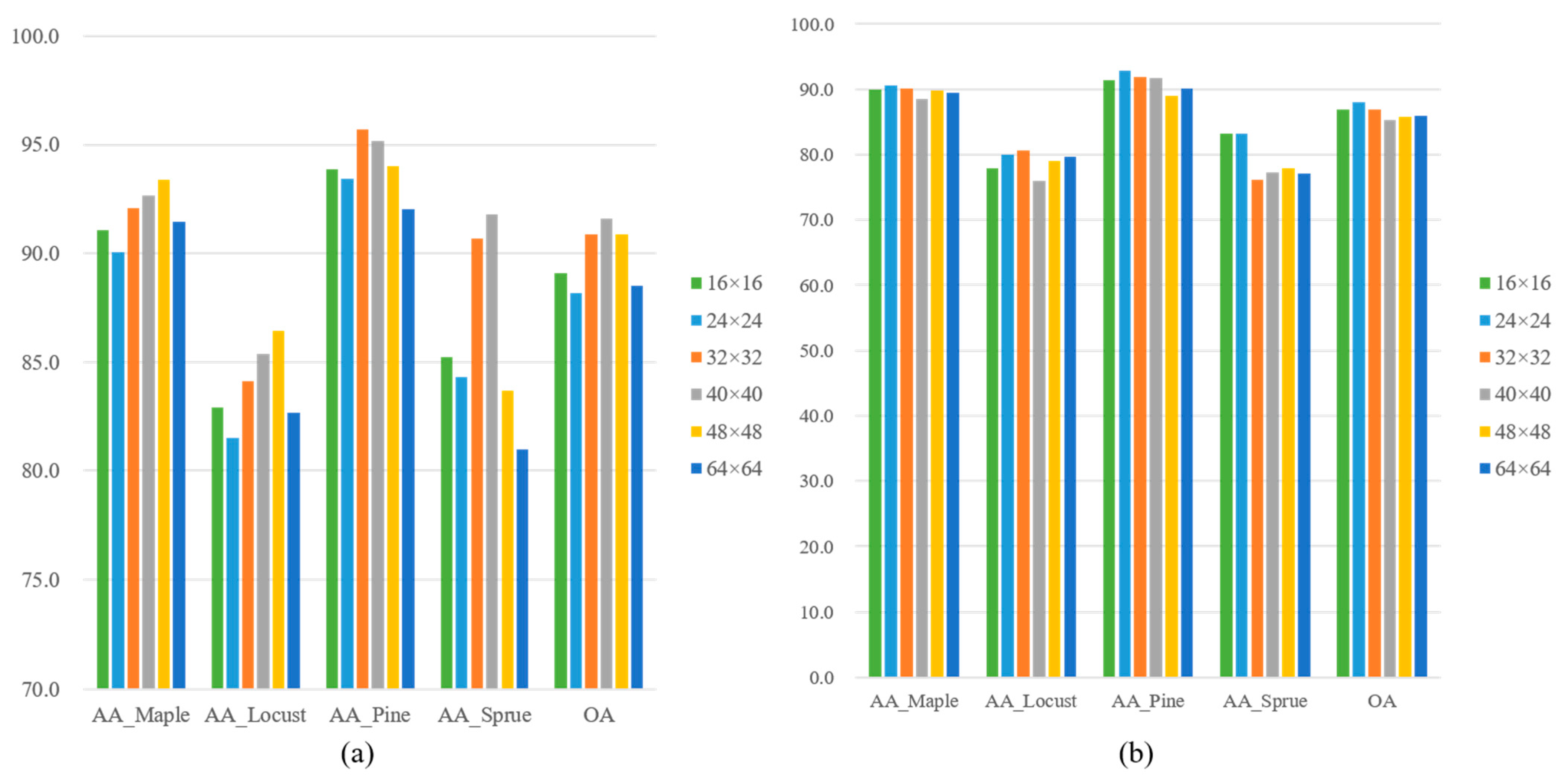
Furthermore, experimental results showed that the size of input samples has impact on the classification accuracy of ResNet-18. In contrast, the OA and kappa values of DenseNet-40 didn’t vary so much with the input sizes as those of ResNet-18. Therefore, it is suggested that the input size of ResNet models can be determined according to the maximum size of all tree crown sample images. Atmospheric correction is unnecessary when ITS classification was conducted using both pansharpened satellite images and airborne LiDAR data.

The use of satellite images with a higher spatial resolution, which can provide sample images with larger input size, would be beneficial for ITS classification, especially for the species with relatively small crown sizes, such as pine and spruce. For example, WorldView-3/4 can be used in further work. Additionally, more training samples could be collected to improve further and validate the networks.