The Driving Forces of Anoplophora glabripennis Have Spatial Spillover Effects

Abstract

Anoplophora glabripennis Motschulsky, 1854 (Asian longhorned beetle) does serious damage to forests. It has a long history and wide distribution area in China and is spreading there and elsewhere. Extreme climate events, such as cold surges and droughts, have had a promotive impact on Anoplophora glabripennis occurrence, but the spatial spillover effect of extreme climate events and other environmental factors on the occurrence of this pest has not yet been clarified. Two indices, namely, Standardized Precipitation Evapotranspiration Index (SPEI) and Low Temperature Index (LTI), were used to quantify the effects of drought and low-temperature freezing damage. Based on spatial panel data modeling, this study calculated the spatial spillover effect of environmental factors on the incidence of Anoplophora glabripennis in 666 counties in China’s central plains from 2002 to 2009. The factors examined included LTI, SPEI, average wind speed, hours of sunlight, Gross Domestic Product (GDP) of regional primary industry, population density, Normalized Difference Vegetation Index (NDVI), and pest control rate. Study results indicated that the impacts of environmental factors on the incidence rate of Anoplophora glabripennis are different. Low-temperature freezing damage, drought, wind speed, and pest control rate had a driving impact on pest incidence rates. Overall, the direct effect accounts for about 85% of the total effect, while the indirect effect accounts for about 15% of the total effect.

1. Introduction

Anoplophora glabripennis Motschulsky, 1854 (Coleoptera: Cerambycidae), also known as Asian longhorned beetle, is one of the main forest pests threatening the health of forest resources around the world. A. glabripennis is native to China and the Korean Peninsula [1]. A. glabripennis had long been a general pest in China, with very few outbreak records. However, since the 1980s, the disease broke out in many areas of China [2]. By the early 1990s, A. glabripennis was reported in most parts of China, except for the western provinces of Qinghai, Tibet and Xinjiang, and Heilongjiang Province. At present in China, A. glabripennis has become one of the major forest pests, and the pest occurs primarily in farmland shelter belts and timber forest areas north of the Yangtze River. Liaoning, Hebei, Henan, Shanxi, Shaanxi, and Shandong provinces and the municipalities of Tianjin and Beijing are high incidence areas of pests [3,4], and pest incidence is vertically distributed from the low-level basins and plains in the east to the high-altitude mountains in the southwest. The outbreak and expansion of A. glabripennis were linked to the nationwide afforestation programs that began in the 1960s. The largest of the tree-planting programs was the Three-North Shelterbelt Forest Program, initiated in the arid regions of northern China in 1978 with the goal of establishing forests on more than 350,000 square kilometers by 2050. The main goal of the Three-North Shelterbelt Forest Program was to increase forest cover and thereby slow desertification and reduce soil erosion [2,3]. In order to improve the ecological environment as soon as possible, Populus dakuanensis Hsu was chosen as the main plantation species, but it was later found that this species was susceptible to A. glabripennis, and the species was too homogeneous. These factors led to the outbreak of A. glabripennis [2]. Between 1980 and 1990, widespread outbreaks of A. glabripennis occurring in Ningxia Province and Inner Mongolia led to the destruction of over 90 million infested trees [5]. A. glabripennis is not considered a pest in Korea as it is uncommon and typically attacks native Acer mono Maxim and Acer truncatum Bunge [1,3,6].

A. glabripennis was detected outside Asia for the first time in 1996 in New York City. After 1996, this species was found in an increasing number of places in North America (Chicago (1998), New Jersey (2002), Toronto (2003), Ontario (2003), Canada (2003), Massachusetts (2008)). In August 2008, a new infestation site was discovered in Worcester, Massachusetts, as the first occurrence in New England [7]. In Europe, since the first record in Austria in 2001, additional infestations have been detected in other countries including France (2003), Germany (2004), Italy (2007), Belgium (2008), The Netherlands (2010), Switzerland (2011), the UK (2012), Finland (2015), and Montenegro (2015). Despite the eradication programs initiated in Europe, A. glabripennis populations are still reproducing and potentially spreading [8,9]. A. glabripennis has caused serious economic losses. In China alone, A. glabripennis causes an estimated annual loss of more than 1.5 billion dollars. If the established populations of A. glabripennis are not eradicated, A. glabripennis may cause more than 600 billion dollars of damage in the United States [10].

A. glabripennis mainly harms broad-leaved tree species, such as eucalyptus, willow, and poplar, and A. glabripennis is more harmful in pure forests than in mixed forests [11]. A. glabripennis has enormous destructive potential because it attacks healthy trees and spends most of its life as a larva, boring inside tree trunks and large branches. This compromises the tree’s vascular system, causes severe damage to the wood’s structural properties, and eventually leads to the death of the attacked trees. Young and old trees are more vulnerable to attack by A. glabripennis, and mature trees are resistant [1]. Although adult beetles can cause twig mortality during their maturation feeding, larvae cause most of the damage as they tunnel through branches and boles [1,12,13]. It produces one to two generations per year in most southern parts of China, and one generation every 2–3 years in the north [14,15]. Generational development of the eggs, larvae, and adults requires initial temperatures of 11.9 ± 1.09, 15.2 ± 1.87, and 13.4 ± 0.30 °C, and an effective accumulated temperature of −75.05 ± 15.17, 958.74 ± 99.95, and 991.05 ± 188.28 °C, respectively. The pest can complete one generation per year when these conditions are satisfied [16].

The occurrence and spread of A. glabripennis are affected by various environmental factors, such as natural environmental factors and socio-economic factors. The pest’s physiological activities and the period and scale of the occurrence are directly affected by meteorological factors [17,18,19]. Egg hatching and larval development are significantly disturbed outside the range of 10–35 °C [15]; larval survival rate, adult wing length, mating behavior, and spawning behavior are significantly influenced by precipitation and humidity [20,21]. The pest’s migration and diffusion patterns are affected by wind speed and wind direction [22,23], and its distribution is also affected by the solar radiation [24]. In addition, eggs, larvae, and pupae can be easily spread along human transportation networks [25,26].

In recent years, under global climate change, the increasingly frequent extreme climate events are often accompanied by pest occurrence [27,28]. Tree wilting caused by drought and low-temperature freezing damage have decreased tree resistance to pests, reduced the population density of natural enemies, and given rise to more favorable living conditions for pests. In addition, significant changes in the effective accumulated temperature also affect the occurrence period and suitable living areas for A. glabripennis.

Most studies of climate change effects on A. glabripennis use species distribution models (SDMs) to monitor the variability and assess the potential distribution [24,29]. Quantifying relationships between distribution and environmental gradients, SDM estimates the geographic locations of pest occurrence spatially [30,31]. Research on the driving factors of pest occurrence have focused primarily on evaluating the growing adaptability and assessing the infestation risk. The methods of such research have typically involved regression analysis [32,33], empirical modeling [14,25], and life table analysis [34,35]. The relationship between environmental factors and pest incidence rate has generally been fitted by linear regression models, and the models ignore the spatial dependencies among factors and do not reveal the extent of spatial spillover effects of factors [36]. The study described in this paper used spatial panel data models to explore the driving effects and spatial spillover effects of different environmental factors, including extreme climate factors, on the incidence of A. glabripennis to better support the prevention and control efforts for this pest.

2. Materials and Methods

In this section, we give a brief introduction of the study area and data sets used in statistical models. Firstly, the incidence of A. glabripennis in each county in the study area was calculated, and then nine environmental factors affecting A. glabripennis were collected, including meteorological factors, social-economic factors, human activities factors, vegetation cover factors, and control and prevention factors. Finally, nine environmental factors were used to measure the influence of natural and human factors on the incidence rate of A. glabripennis, whose direct, indirect, and total effects were estimated by spatial panel data models.

2.1. Study Area

The study area, shown in Figure 1, is located at 105.5° E–122.7° E, 29.7° N–42.7° N and includes 666 counties within two municipalities (Beijing and Tianjin) and six provinces (Hebei, Henan, Shanxi, Shandong, Shaanxi, and Anhui) with a total area of about 1,041,600 km². This area lies mainly within the North China Plain, Taihang Mountains, and Loess Plateau, with a terrain that includes basins, plains, hills, and mountains. The area is in a warm-temperate zone and its main climate type is temperate monsoon (cold and dry in winter, hot and rainy in summer) with an average annual temperature range of 8–20 °C and annual precipitation of 300–1000 mm. The vegetation cover in the study area is dominated by broad-leaved forest.

2.2. A. glabripennis Incidence Calculation

Statistical data on the incidence of A. glabripennis in the study area during 2002–2009 was provided by the National Bureau of Forestry and Grassland Forest Pest Control Station (https://www.forestpest.cn/, accessed on 6 July 2017). The pest incidence rate was obtained by dividing “pest occurrence area” by “pest monitored area” from the statistical data. Some counties in the study area had a reported zero incidence rate. This is possibly due to omission or loss of samples, lack of data collection, and/or randomness of the sampling process. A. glabripennis is native to China and has been occurring in the study area for many years, so the pest incidence rates can be considered to have similar distribution patterns in adjacent areas within counties. Thus, in this study, we adjusted the incidence for counties with a reported zero incidence rate with a multi-level Bayesian model by using the method of Besage, York, and Mollie to “fill in” the zero value [37]. The core idea of the model is to improve the accuracy of the data through the spatial relationship between a certain county and its adjacent counties, and the adjusted logarithm of the i-th county meets (1):

$$\log ({\theta }_i)=\alpha +V_i+{\epsilon }_i$$

(1)

where $\alpha$ is the overall risk level of the incidence rate, $V_i$ is the spatial aggregation, and ${\epsilon }_i$ is the spatial heterogeneity that obeys a normal distribution $({\epsilon }_i~N(0,{\sigma }_i^2))$. $V_i$ satisfies the conditional autoregressive range [38] model hypothesis:

$$p(v_i|v_j,j\ne i)\sim N(\overline{v},\frac{{\sigma }_v^2}{n_i})$$

(2)

$$v_i={\displaystyle {\sum }_s\frac{{\delta }_i{v}_s}{n_i}}$$

(3)

where $n_i$ is the number of elements in the adjacent space set (${\delta }_i$) of the i-th county, and ${\sigma }_v$ represents the changing degree of $V_i$ and obeys the gamma distribution $1/{\sigma }_v~Gamma(0.5,0.0005)$ as a prior distribution. The parameter estimation process was completed in WinBugs1.4 (https://www.mrc-bsu.cam.ac.uk/software/bugs/the-bugs-project-winbugs/, accessed on 20 December 2017), and the average posterior distribution of adjusted the incidence of A. glabripennis was obtained by Markov chain Monte Carlo (MCMC) simulation iteration after annealing.

2.3. Environmental Factors and Variables

In this section, the Standardized Precipitation Evapotranspiration Index (SPEI) and Low Temperature Index (LTI) are calculated to quantify drought and low-temperature freezing damage, respectively. Nine proxy variables were selected to describe the environmental factors affecting the incidence of A. glabripennis.

2.3.1. Standardized Precipitation Evapotranspiration Index

The standardized precipitation evapotranspiration index (SPEI) is a drought-assessment index based on precipitation and temperature variability [39]. SPEI considers both the influence of evaporation and temperature on drought [40] and has been widely used for analyzing drought trends [41], estimating crop yields [42], and characterizing the relationship between SPEI and meteorological factors [43]. This study calculated the SPEI value for each county on a one-month time scale with the monthly precipitation, monthly temperature, and station latitude data for 115 meteorological stations in the study area during the years 2002–2009 [44]. The annual average of the monthly SPEI value was used to reflect the average degree of drought in a year [45]. The calculation process as done in the program R with the SPEI package (https://cran.r-project.org/web/packages/SPEI/index.html, accessed on 4 February 2018) [46].

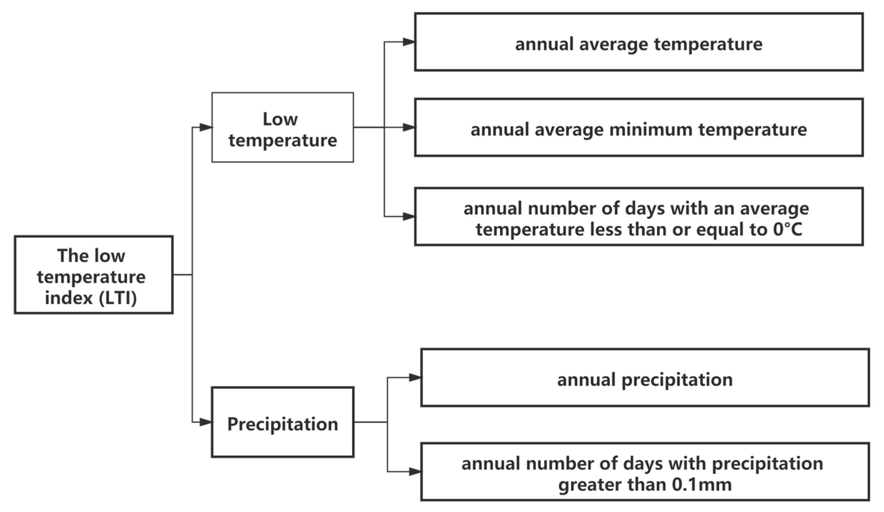
2.3.2. Low Temperature Index

The low temperature index (LTI) was used to quantify extreme low temperatures and frozen rain, snow, frost, and other events caused by cold air activities. Combined with the other calculation method of low-temperature freezing damage assessment indices [47,48,49,50], five meteorological factors available for 115 meteorological stations in the study area for 2002–2009 were used to calculate LTI in this study: annual average temperature, annual average minimum temperature, annual precipitation, annual number of days with an average temperature less than or equal to 0 °C, and annual number of days with precipitation greater than 0.1 mm. We first performed z-score standardization on the five meteorological factors, and then determined the weight coefficient of each meteorological factor through the analytic hierarchy process (Appendix A):

$$LTIValue=0.153\times A+0.087\times B-0.23\times C-0.129\times D-0.4\times E$$

(4)

where A is the annual average temperature, B is the annual average minimum temperature, C is the annual precipitation, D is the annual number of days with precipitation greater than 0.1 mm, and E is the annual number of days with an average temperature less than or equal to 0 °C. The coefficients were obtained by using the analytic hierarchy process (AHP) based on the relative important judgment matrix of the five meteorological factors. Matrixes were passed through the consistency ratio test (CR < 0.1).

2.3.3. Environmental Factors and Proxy Variables

To measure the influence of natural and human socio-economic environmental factors on the occurrence and spread of A. glabripennis, we selected nine environmental factors (available for each county in 2002–2009) as proxy variables for the environmental factors (Figure 2). The influencing factors on the occurrence of A. glabripennis mainly include natural factors and human socio-economic factors. In terms of natural factors, on the one hand, it includes tree species hosted by A. glabripennis; on the other hand, it mainly includes various meteorological factors. Due to the large area of the research, we used the normalized difference vegetation index (NDVI) to characterize the tree species in this study. In terms of meteorological factors, this study especially considered the extreme meteorological index and the meteorological value in the key month, so the indicators included extreme drought index, extreme freezing rain and snow index, wind speed, sunshine, and temperature. In terms of human socio-economic factors, it included regional Gross Domestic Product (GDP), population density, traffic density, and control rate of A. glabripennis. Natural environmental conditions were characterized by LTI, SPEI, average wind speed, and sunlight hours; socio-economic factors and human activities were represented by primary industry GDP and population density, respectively; vegetation cover was represented by NDVI; and pest control and prevention were characterized by the pest control rate (Figure 2).

The meteorological data for all four natural environmental proxy variables came from the surface meteorological observation site data of the National Meteorological Information Center (http://data.cma.cn/, accessed on 26 July 2017), and was spatialized to the individual counties by using Kriging interpolation. The socio-economic data came from China’s County Social and Economic Data Statistical Year book, City Statistical Year book, and Regional Economic Statistical Yearbook for each of the study year. The NDVI data came from the Chinese Academy of Sciences Scientific Data Cloud (http://www.csdb.cn/, accessed on 26 July 2017).

2.4. Spatial Panel Data Models

This study used three spatial panel data models for testing and modeling in the study area [51]: spatial lag model (SLMp), spatial error model (SEMp), and spatial Durbin model (SDMp).

The SLMp model adds the spatial lag term of the interpreted variable to the general panel data model, indicating that the explanatory variable on a spatial unit is affected by the explanatory variable of the adjacent spatial units. The SEMp model adds spatially correlated error terms, and the error term of a spatial unit model is considered to be affected by the error term of the adjacent spatial units. The SDMp model synthesizes the characteristics of SLMp and SEMp, and the intensity affected by the adjacent spatial units is represented by the spatial weight matrix:

$$Y_{it}=\rho W{Y}_{it}+\beta X_{it}+{\lambda }_t+{\mu }_i+{\epsilon }_{it},{\epsilon }_{it}\sim N(0,{\delta }^2{I}_N)$$

(5)

$$Y_{it}=\beta X_{it}+{\lambda }_t+{\mu }_i+(\kappa W{\phi }_{it}+{\epsilon }_{it}),{\epsilon }_{it}\sim N(0,{\delta }^2{I}_N)$$

(6)

$$Y_{it}=\rho W{Y}_{it}+\beta X_{it}+W{X}_{it}\alpha +{\lambda }_t+{\mu }_i+{\epsilon }_{it},{\epsilon }_{it}\sim N(0,{\delta }^2{I}_N)$$

(7)

where $Y_{it}$ is the pest incidence rate in the t-th year of the i-th county; $X_{it}$ represents the value of proxy variables in the t-th year of the i-th county; $\beta$ reflects the extent to which proxy variables affect the pest incidence rate; $W$ is the 0–1 spatial weight matrix, and $W_{ij}=1$ when the i-th county and the j-th county are adjacent; ${\lambda }_t$ and ${\mu }_i$ represent temporal and spatial effects, respectively; ${\phi }_{it}$ is a spatial error term; $\kappa$ is the spatial error autocorrelation coefficient, measuring the degree of influence that the error of observations in adjacent counties affects the observed values in a given county; and ${\epsilon }_{it}$ is a random error term obeying a normal distribution.

Two Lagrange multipliers—LM_Lag and LM_Error—and two robust Lagrange multipliers—R-LM_Lag and R-LM_Error—were used to determine whether the spatial lag (SLMp) and spatial error effects (SEMp) were significant. If the test results showed that only one effect was significant, then the corresponding spatial effect model was built; if the test results showed that the spatial lag and spatial error effects were either both significant or both not significant, then the SDMp model was built. After that, the Wald or LR test was used to determine whether the SDMp model could be simplified to the SLMp or SEMp model. In addition, in order to consider the effects changing with the location and time series of proxy variables on the pest incidence rate, the significance of spatial fixed effects, time-period fixed effects, and spatial and time-period fixed effects were tested simultaneously during the process of model selection.

After selecting the appropriate model, in order to better reflect the direct and spatial spillover effects of proxy variables in the model, a decomposition of the total effects was performed. A flowchart is presented to give the estimation process of the spatial panel data models described above, selecting the proper model to explore the direct and spatial spillover effect on the pest incidence rate (Figure 3).

The direct effect characterized the impact on the pest incidence rate in a county of that county’s proxy variables. The spatial spillover effect (also called the indirect effect) characterized the impact on the pest incidence rate in adjacent counties of that county’s proxy variables. The models were built using the Matlab package provided by Elhorst [52]. Additionally, to check the stability of the data and avoid model pseudo-regression, we used the LLC, IPS, Fisher ADF, and Fisher PP test methods to perform unit root testing on the data [53], and the cointegration relationship between variables was calculated using the Kao panel test method (Appendix B) [54].

3. Results

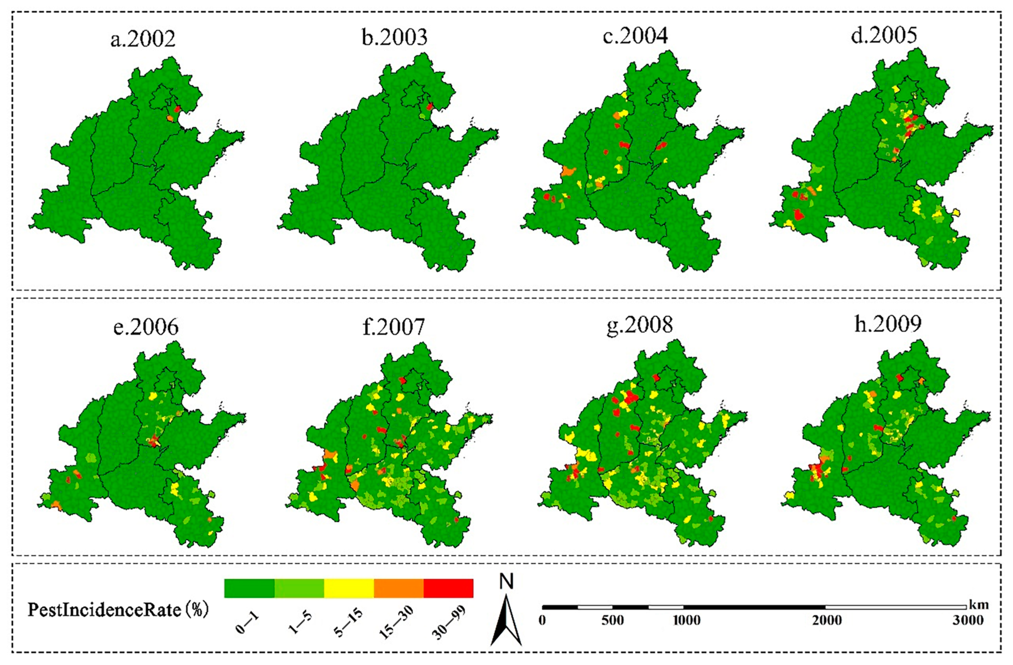
3.1. Spatiotemporal Patterns of the Incidence of A. glabripennis in 2002–2009

The incidence of A. glabripennis during 2002–2009 showed some spatial concentration in study areas with a high pest incidence rate, and the trend of the concentration was relatively stable. The high incidence areas were mainly concentrated around Handan City in the southern part of Hebei Province, Cangzhou City in the eastern part of Hebei Province, Xianyang and Baoji cities in the central part of Shaanxi Province, and Xinzhou City in the northern part of Shanxi Province. The largest and most widespread incidence of pests occurred in 2007 and 2008. Pest incidence in 2005 and 2009 was moderate severe in most areas. In 2004 and 2006, pests only occurred in individual counties (Figure 4).

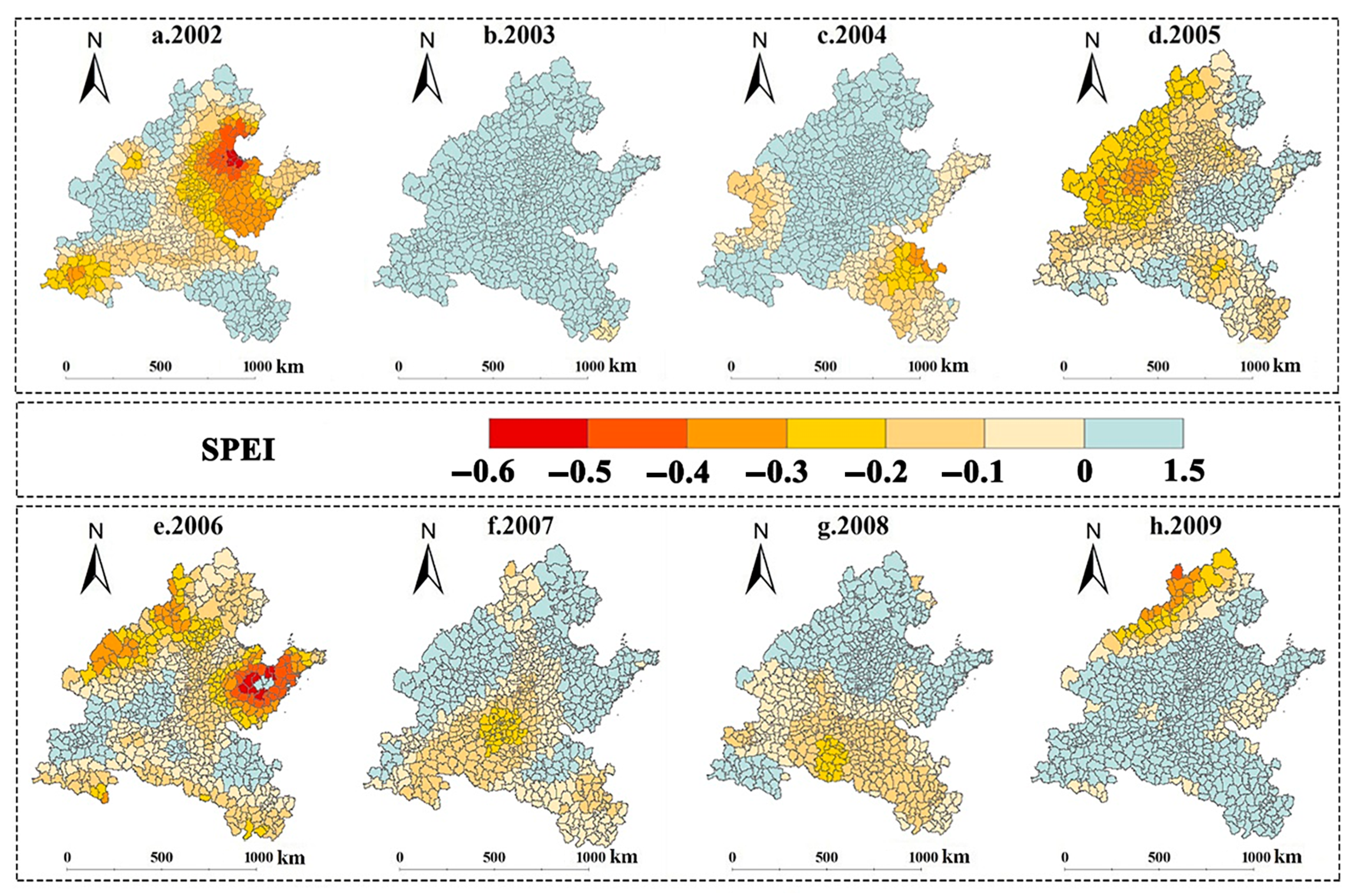
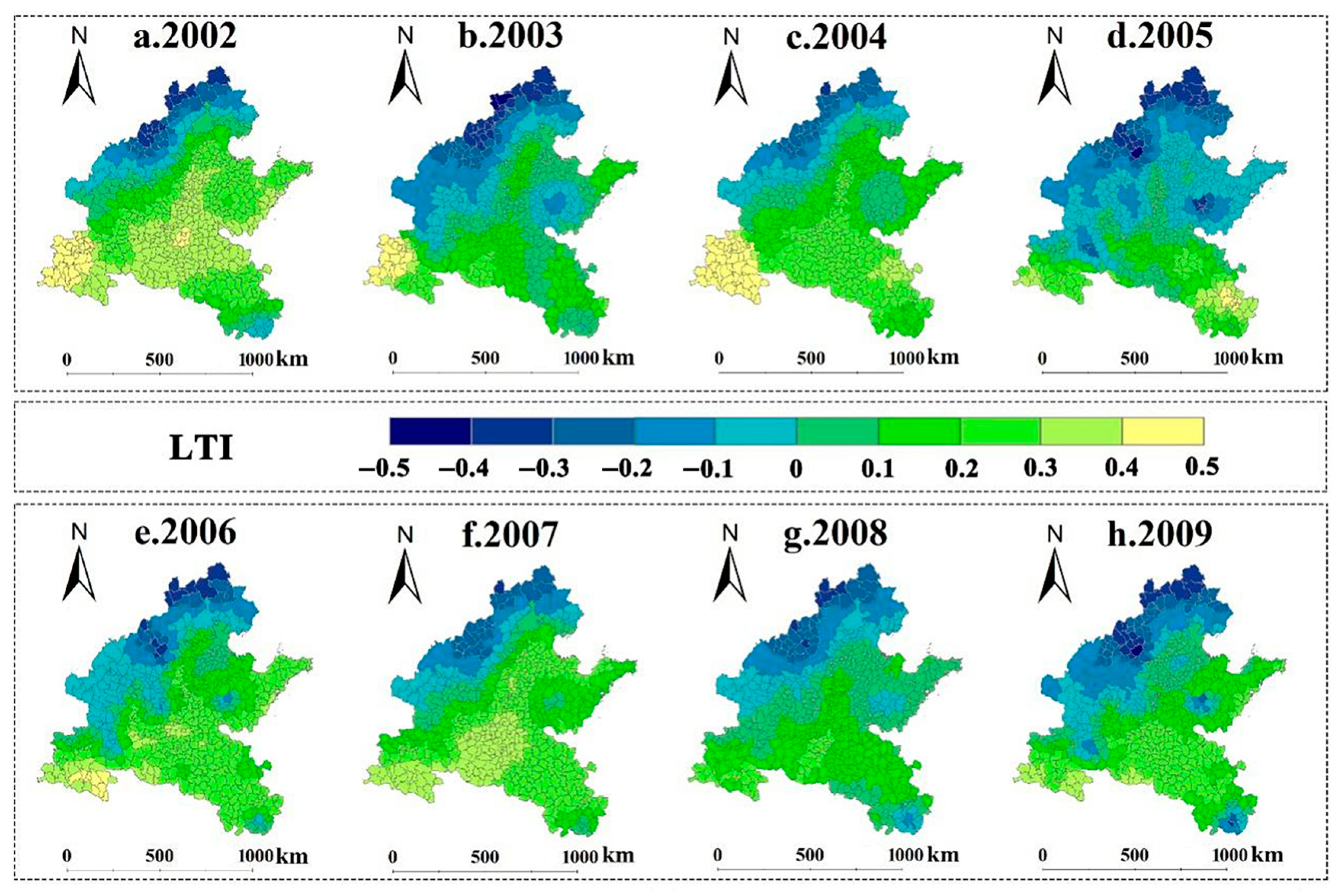
3.2. Spatiotemporal Patterns of SPEI and LTI in 2002–2009

The description of the pest incidence rate and nine proxy variables is shown in

Table 1. Distribution of the incidence rate of A. glabripennis and environmental factors.

Variable	Mean	StdDev	Min	Max
PIR	1.26	7.19	0	99.64
LTI	0.11	0.19	−0.44	0.45
SPEI	0.05	0.26	−0.56	1.01
AWS	2.24	0.46	1.24	4.69
SH	2157.13	365.22	1129.56	2952.18
PIGDP	9.71	11.49	0.23	126.73
PD	550.98	531.5	6.06	5324.12
NDVI RD	0.54 17.19	0.1 22.46	0.22 0.12	0.83 209.34
PCR	9.41	27.91	0	100

Note: PIR, pest incidence rate (%); LTI, low temperature index (%); SPEI, standardized precipitation evapotranspiration index (%); AWS, average wind speed (m/s); SH, sunlight hours(hours); PIGDP, primary industry gross domestic product (hundred-million US dollars); PD, population density(pop./km²); NDVI, normalized difference vegetation index; RD, road density (km/km²); PCR, pest control rate (%).

. Drought varied with latitude and longitude but tended to aggregate spatially (Figure 5). In 2002, slight and moderate drought occurred in Tianjin, Cangzhou City in Hebei Province, Xi’an and Hanzhong cities in Shaanxi Province, Binzhou and Dezhou cities in Shandong Province, and the central part of Shandong Province. In 2003, there was no obvious drought in the study area. From 2004 to 2006, the drought intensity increased gradually and shifted spatially from central Shaanxi Province to Shandong Province. In 2007–2009, drought conditions were slight. In 2007–2008, there was only a slight drought in Henan and Anhui Province. In 2009, slight and moderate droughts occurred in northern Shanxi Province. Overall, the drought intensity of the study area was relatively serious in 2002, 2005, and 2006 and relatively slight in other years.

LTI values during 2002–2009 indicated the distribution of low-temperature freezing damage in the study area (Figure 6). Most of the low-LTI-value areas were concentrated in the northwestern counties, due to their relatively high latitude and elevation. In addition, during 2002–2009, the LTI for Jining City in Shandong Province decreased and increased repeatedly. After the low-temperature freezing damage appeared in 2003, 2005, and 2006 for Jining City, the LTI decreased again in 2008–2009. Weinan City in Shaanxi Province had a lower LTI value in 2005 and 2009. Additionally, Huangshan City in Anhui Province showed a lower LTI value in 2008 and 2009. Overall, the low-temperature freezing damage that occurred in 2005 and 2009 was relatively serious, and relatively slight in other years.

3.3. Spatial Spillover Effects of Proxy Variables on A. glabripennis

In this section, the estimation results of the spatial panel data model are presented according to the process shown in Figure 3, and the direct and indirect (spatial spillover) effects of environmental factors are characterized by spatial panel data models.

The test results for the no-fixed effects and three fixed effects all significantly rejected for LMError and R-LMError (

Table 2. Panel data model estimation results without spatial interaction.

	Ordinary Least Square (OLS)	Spatial Fixed Effects	Time-Period Fixed Effects	Spatial and Time-Period Fixed Effects
R2	0.0970	0.0880	0.0899	0.0761
σ2	46.7350	32.5133	46.5311	32.3688
LMLag	57.1994 ***	43.1199 ***	49.7640 ***	38.9140 ***
R- LMLag	0.3950	2.7550	0.7129	1.8456
LMError	65.2111 ***	51.9631 ***	57.1980 ***	45.8077 ***
R-LMError	8.4067 ***	11.5982 ***	8.1469 ***	8.7393 ***

Note: *** indicates p < 0.01.

), so the model at least needed to contain the autocorrelation residual term of the SEMp model. Next, to test the different fixed effects, the likelihood ratio test (LR test) was performed. The results showed that the model needed to consider the fixed effects in space (1933.9996, p < 0.001) and time (24.0674, p < 0.001) [52].

To verify whether the SDMp model could be simplified to the SEMp model, the Wald test and LR test were performed (

Table 3. Wald test and LR test results of the SDMp model.

	Spatial Fixed Effects	Time-Period Fixed Effects	Spatial and Time-Period Fixed Effects
Wald_spatial_lag	21.7455 *** (p = 0.0097)	28.5366 *** (p = 0.0008)	19.3922 ** (p = 0.0221)
Wald_spatial_error	13.7424 (p = 0.1318)	22.3532 * (p = 0.0780)	13.1501 (p = 0.1559)
LR_spatial_lag	21.5087 ** (p = 0.0106)	28.3853 *** (p = 0.0008)	19.2121 ** (p = 0.0234)
LR_spatial_error	12.8898 (p = 0.1053)	22.1075 * (p = 0.0850)	13.0737 (p = 0.1593)

Note: *** indicates p < 0.01; ** indicates p < 0.05; * indicates p < 0.10.

). In three different fixed effect models, the null hypothesis that simplified the SDMp model to the SEMp model could not be rejected at a high level of significance. Meanwhile, the random effect was also rejected according to the Hausman test (68.5685, p < 0.001). Therefore, an SEMp model with a spatial or time-period fixed effects was chosen.

The results of using three different fixed effects in SEMp modeling is given in

Table 4. Different fixed effects of the SEMp model estimation results.

	Spatial Fixed Effects	Time-Period Fixed Effects	Spatial and Time-Period Fixed Effects
LTI	−1.5361 **	1.4341	−1.4658
SPEI	−1.1384 ***	−0.3138	−1.3558 **
AWS	1.6551 ***	−0.0062	1.6066 **
SH	−0.0046 ***	0.0010	−0.0062 ***
PIGDP	−0.0100	−0.0467 ***	−0.0255 *
PD	−0.0018	−0.0002	−0.0024 *
NDVI	3.5612	−1.6425	−7.9150
RD	5.0770	0.0045	5.3191
PCR	0.0727 ***	0.0794 ***	0.0730 ***
σ2	36.5820	45.8413	36.5246
R2	0.3716	0.1007	0.3745
CorrectedR2	0.0899	0.0879	0.0761
LogL	−16,727.723	−17,758.275	−16,795.896
Spat.error.	0.1521 ***	0.1550	0.1483 ***

Note: *** indicates p < 0.01; ** indicates p < 0.05; * indicates p < 0.10. The meaning and unit of all variables are the same as that of Table 1.

. In comparing the loglikelihood (LogL) values, the corrected R-square (CorrectedR2) values and the significance of each proxy variable coefficient and Spat.error, an SEMp model that incorporates spatial fixed effects appears to best explain the problems studied in this study. Furthermore, the spatial differences in environmental factors across the study area and the short time span involved (2004–2009) are additional reasons for choosing the spatial fixed effects model.

According to the estimation process above, an SEMp model that incorporates spatial fixed effects was chosen finally. To characterize the different driving effects of nine proxy variables on the pest incidence rate, we calculated the direct effects, indirect effects, and total effects of environmental factors (

Table 5. Effects of environmental factors on the incidence rate of A. glabripennis.

Variable	Direct Effect	Indirect Effect	Total Effect
LTI	−1.5319 *	−0.2671 *	−1.7990 *
SPEI	−1.1484 ***	−0.2003 ***	−1.3487 ***
AWS	1.6507 ***	0.2878 ***	1.9358 ***
SH	−0.0046 ***	−0.0008 ***	−0.0054 ***
PIGDP	−0.0098	−0.0017	−0.0115
PD	−0.0018	−0.0003	−0.0021
NDVI	3.5110	0.6131	4.1254
RD	5.1350	0.9006	6.0356
PCR	0.0730 ***	0.0127 ***	0.0857 ***

Note: *** indicates p < 0.01; * indicates p < 0.10. The meaning and unit of the variable are the same as that of Table 1. “Direct effect” is the impact of the environmental factor on the pest incidence rate in the given county; “Indirect effect” is the impact of the environmental factor on the pest incidence rate in adjacent counties; and “Total effect” is the total impact of the environmental factor on the pest incidence rate. The coefficient estimation values of effects represent the varying percentage of the pest incidence rate with 1 unit increasement of the corresponding environmental factor (e.g., the incidence rate of A. glabripennis will decrease 1.5319% (direct effect) and 0.2671% (indirect effect) with a 1% increasement of LTI, respectively).

). The pest incidence rate was mainly affected by LTI, SPEI, average wind speed, and pest control rate, while the sunlight hours showed a significant but weak effect and the primary industry GDP, the population density, and NDVI did not show significant driving effects in this study.

The impacts of environmental factors on the incidence rate of A. glabripennis are different (Table 5). The influences of meteorological factors (LTI, SPEI, AWS, and SH) on A. glabripennis passed the significance test, but the influences of social economy factors (PIGDP, PD, and RD) on A. glabripennis were not significant. Overall, the direct effect accounted for about 85% of the total effect (direct effect/total effect), while the indirect effect accounted for about 15% of the total effect (indirect effect/total effect).

The direct, indirect, and total effect coefficients of the SPEI are significant at the 1% level (−1.1484, −0.2003, and −1.3487, respectively), and the direct effect is obvious. Compared with LTI (−1.5319, −0.2671, and −1.5406, respectively), the spatial spillover effect of SPEI is relatively smaller but shows a higher level of significance. If the drought tends to be serious with a 1% reduction in the SPEI for a given county, the pest incidence rate will increase by 1.15% and 0.2% within that county and in adjacent counties, respectively.

The direct, indirect, and total effect coefficients of the AWS are significant at the 1% level (1.6507, 0.2878, and 1.9358, respectively). If the average wind speed from May to August increases with 1 m/s for a given county, the pest incidence rate will increase by 1.65% and 0.29% within that county and in adjacent counties, respectively.

4. Discussion

This study analyzed the occurrence distribution of A. glabripennis in 666 counties from 2002 to 2009, and the pest presented a temporal and spatial concentration pattern. The spatial spillover effects caused by the occurrence of pests in a given country had produced the possibility of occurrence in adjacent counties. Since the initiation of China’s “Three North” shelter belt project from 1979, the occurrence and spread of A. glabripennis has been rampant in the central and eastern parts of China [55]. The counties with low incidence rates were distributed around the high incidence rate counties, and the concentration trend of high incidence rate counties was stable in 2004–2009. The positive estimate of the error term coefficient in the panel model reflected the concentration of a high pest incidence rate. When a county had a severe pest occurrence in its adjacent counties, the occurrence in that county was also severe. This makes the pests rapidly expand in the forest of single tree species with the ever-expanding plantation resources in China.

By using an SEMp model with a spatial fixed effect, we characterized the direct effects and spatial spillover effects of different environmental factors through their proxy variables on the pest incidence rate. The pest incidence rate was found to be affected by proxy variables both in a given county and adjacent counties, especially variables of drought, low-temperature freezing damage, and wind speed.

Drought had a positive effect on the occurrence of A. glabripennis, but its spatial spillover effects were not obvious. In general, the high temperatures and low precipitation rates caused by drought will limit the growth and distribution of host trees, and the drought affects pest indirectly by affecting the host vegetation [56,57]. Drought weakens the host trees, and it will make host trees emit more attractive compounds to pests [58]. In this study, pest occurrence occurred in Fengxiang, Jingyang, Chengcheng, Fu, and Gaoling counties in Shaanxi Province in 2004, when a slight drought occurred and the SPEI values for those counties were 0.6–0.8 lower than those in 2003. Then, in 2005, the drought conditions in these counties were further severe and the SPEI values declined by 0.11, 0.100, 0.16, 0.13, and 0.09, respectively. In this same year, the pest incidence rates in Fengxiang and Jingyang counties increased by 49.48% and 21.89%, respectively. In addition, the impact of drought on pest occurrence may not always be immediate. For example, the severe 2006 drought in central Shandong Province did not lead to pest occurrence in that year, but outbreaks did occur in Yishui County and Shouguang City in 2007 and 2008. The 2006 drought in Cangzhou and Datong cities in Shanxi Province was followed by pest occurrence in 2007–2009.

The spatial spillover effect of low-temperature freezing damage was generally greater than that of other proxy variables examined in this study. Natural disasters, such as cold waves, freezing rain, frost, and heavy snowfall, can seriously damage forest ecosystems and quickly reduce tree vigor, resulting in the secondary occurrence of pests, and it usually affects a wide range of areas [59]. Conversely, the positive effects of the LTI did not show a high level of significance (10%), because the low-temperature freezing damage has different effects at different times on pests. When larvae are wintering, their cold resistance significantly depends on the choice of host tree [60], and the “cold spring” climate phenomenon may inhibit the growth of wintering larvae and thereby reduce pest occurrence in following years.

Wind speed showed certain spatial spillover effects on pest incidence rates. The wind has a direct influence on the migration, distribution, and growth of the pest. Related experiments have found that adult pests will require wind when they are looking for food, spouses, and habitats. Their start-up time, angle, and distance of flight are all affected by the wind [61,62]. Wind accelerates the spread of this pest. The pattern of pest occurrence in the counties near Handan City in Hebei Province during 2004–2007 is illustrative of this process. The average annual wind speed in these counties was 2–3 m/s throughout 2004–2007. In 2004, the first pest occurrence occurred in Xiajin and Pingyuan counties. In 2005, round these two counties, seven other counties reported low or medium pest incidence rates, which were adjacent to one another. In 2006, the pest incidence rates in three of those seven counties (Wei, Quzhou, and Guantao counties) rose from 23.55%, 17.56%, and 9.57% to 44.44%, 49.41%, and 49.45%, respectively. Meanwhile, four additional counties in the adjacent area had pest occurrence. In 2007, among all these former counties, four counties had significantly higher pest incidence rates compared to the previous three years.

Hours of sunlight showed only a weak inhibiting effect on the occurrence of the pest in this study. Previous research has proved that pests are more likely to occur in areas with sufficient sunlight conditions. In addition, the influence of light on biological rhythms and physiological activities of pests is often reflected in a special time range, so the cumulative hours of sunlight in the whole year is not enough to constitute a driving effect on pest occurrence. Normally, light is used to explore its effect on the survival and mortality rate of different stage of pests and has obtained different conclusions [63,64].

Human activities, represented by primary industry GDP, population density, and road density in this study, did not show significant spillover effects on the occurrence of the pest. However, population changes have facilitated the invasion, development, and spread of pests [38,65]. The expansion of urban areas reduces the available living space, population, and biodiversity of natural enemies [66]. Conversely, the construction of farmland shelter belts has enhanced the living environment for the natural enemies on the edges of farming areas, to some extent, which inhibits pest occurrence in these areas [67]. In addition, although changes in the natural environment and the improvement of prevention-and-control technology have facilitated prevention and eradication of the pest [68], the pest’s adaptability is strong, and its spread can be accelerated by human activities along traffic lines. In this study, road density did not have a significant impact, which is due to the fact that there was no significant change in road density in the study area from 2002 to 2009. However, in areas where no pests occur, the invasion of this pest is obviously affected by transportation [69]. Despite high control rates in our study, the high incidence rate areas, such as Handan, Xianyang, and Jinzhong cities, were continuously affected by pests. This shows the seriousness of the pest epidemic, and risks of its spread need further research [70].

There are some limitations to our study. Firstly, it should be noted that the positive and negative “driving effects” in this study only represented statistical correlations not causal relationships between environmental variables and pest incidence rate. The interactions among environmental variables and the specific mechanism of the effects on pest occurrence and spread need to be further explored. Secondly, the incidence of A. glabripennis in this study is annual statistical data. We did not consider the number of generations of the pest. On the one hand, in most of the research counties, A. glabripennis occur once a year [71,72,73,74,75,76,77,78,79,80]; on the other hand, the whole study area (including 666 counties) is too large, and it is hard to collect the generation of the pest in each county. In the follow-up study, we will focus on the selection of some representative counties, and collect the occurrence of generations.

5. Conclusions

Using data on pest incidence rates and environmental factors for 666 counties within six provinces and two municipalities in China, this study explored the spatial and temporal distribution of the pest incidence rate and the driving forces of the environmental factors from 2002 to 2009. The results showed a spatial concentration on the pest incidence rate in the study area, and the high incidence rate showed a stable concentration trend. Environmental variables had both direct effects and spatial spillover effects on the pest incidence rate in a given county, with low-temperature freezing damage, drought, wind speed, and pest control rates having a significant influence. Both drought and low-temperature freezing damage had positive promoting effects on the pest incidence rate with spatial spillover effects. Overall, the direct effect accounts for about 85% of the total effect, while the indirect effect accounts for about 15% of the total effect. The pest control rate also had a positive coefficient in the model, which indicates the pest may recrudesce when the prevention and control practices are not thorough. The occurrence of regional extreme climatic events and the effect of wind can promote the occurrence of A. glabripennis to a certain extent. Combining the unique biological characteristics of A. glabripennis and the unique driving conditions of the outbreak area, a scientific and timely prediction and control method system can be formulated to provide support and guarantee for healthy and sustainable development of forest.

References

1. Lingafelter, S.W.; Hoebeke, E.R. Revision of the Genus Anoplophora (Coleoptera: Cerambycidae); Entomological Society of Washington: Washington, DC, USA, 2002. [Google Scholar]
2. Luo, Y.; Li, J. Bionomics and occurrence of Anoplophora glabripennis (Motschulsky). Plant. Quar. 1999, 1, 7–9. [Google Scholar]
3. Haack, R.A.; Hérard, F.; Sun, J.; Turgeon, J.J. Managing invasive populations of Asian longhorned beetle and citrus longhorned beetle: A worldwide perspective. Annu. Rev. Entomol. 2010, 55, 521–546. [Google Scholar] [CrossRef] [Green Version]
4. Wu, W.W.; Jiang, S.N. The glabripennis species group of the genus Anoplophora in China (Coleoptera: Cerambycidae). Acta Entomol. Sin. 1998, 41, 284–290. [Google Scholar]
5. Pan, H.Y. Review of the Asian Longhorned Beetle Research, Biology, Distribution and Management in China; Forest Health and Biosecurity Working Papers; Forest Resources Development Service, Forest Resources Division, FAO: Rome, Italy, 2005; pp. 41–44. [Google Scholar]
6. Golec, J.R.; Li, F.; Cao, L.; Wang, X.; Duan, J.J. Mortality factors of Anoplophora glabripennis (Coleoptera: Cerambycidae) infesting Salix and Populus in central, northwest, and northeast China. Biol. Control 2018, 126, 198–208. [Google Scholar] [CrossRef]
7. Hu, J.; Angeli, S.; Schuetz, S.; Luo, Y.; Hajek, A.E. Ecology and management of exotic and endemic Asian longhorned beetle Anoplophora glabripennis. Agr. For. Entomol. 2009, 11, 359–375. [Google Scholar] [CrossRef]
8. Javal, M.; Roques, A.; Haran, J.; Hérard, F.; Keena, M.; Roux, G. Complex invasion history of the Asian long-horned beetle: Fifteen years after first detection in Europe. J. Pest Sci. 2019, 92, 173–187. [Google Scholar] [CrossRef]
9. Xu, T.; Teale, S.A. Chemical Ecology of the Asian Longhorn Beetle, Anoplophora glabripennis. J. Chem. Ecol. 2021, 47, 489–503. [Google Scholar] [CrossRef]
10. Nowak, D.J.; Pasek, J.E.; Sequeira, R.A.; Crane, D.E.; Mastro, V.C. Potential effect of Anoplophora glabripennis (Coleoptera: Cerambycidae) on urban trees in the United States. J. Econ. Entomol. 2001, 94, 116–122. [Google Scholar] [CrossRef]
11. Wang, Z.G.; Su, Z.; Liu, M.H.; Zhao, Y.M.; Zhang, G.; Cui, Z.R.; Dan, H.L.; Chen, X.M. Comparision of the Resistant Characteristics of Populus alba var. pyramidalis and Populus deltoides cl. Beikang to Damages against Anoplophora glabripennis (Coleoptera: Cerambycidae). Sci. Silvae Sin. 2018, 54, 89–96. [Google Scholar] [CrossRef]
12. Haack, R.A.U.F.; Law, K.R.; Mastro, V.C.; Ossenbruggen, H.S.; Raimo, B.J. New York’s battle with the Asian long-horned beetle. J. For. 1997, 95, 11–15. [Google Scholar]
13. Li, H.; Yu, F.; Bi, Y.; Wang, Z. Reviews on the serious wood-boring pest Anoplophora glabripennis in forestry of China. For. Ecol. Sci. 2020, 35, 1–9. [Google Scholar]
14. MacLeod, A.; Evans, H.; Baker, R. An analysis of pest risk from an Asian longhorn beetle (Anoplophora glabripennis) to hardwood trees in the European community. Crop Prot. 2002, 21, 635–645. [Google Scholar] [CrossRef]
15. Keena, M.A. Effects of temperature on Anoplophora glabripennis (Coleoptera: Cerambycidae) adult survival, reproduction, and egg hatch. Environ. Entomol. 2006, 35, 912–921. [Google Scholar] [CrossRef] [Green Version]
16. Yang, Z.M.; Wang, X.; Yao, W.S.; Chu, X.M.; Li, P. Generation differentiation and effective accumulated temperature of Anoplophora glabripennis (Motsch.). For. Pest Dis. 2000, 19, 12–14. [Google Scholar] [CrossRef]
17. Bancroft, J.; Smith, M. Dispersal and influences on movement for Anoplophora glabripennis calculated from individual mark-recapture. Entomol. Exp. Appl. 2005, 116, 83–92. [Google Scholar] [CrossRef]
18. Faccoli, M. Effect of weather on Ips typographus (Coleoptera Curculionidae) phenology, voltinism, and associated spruce mortality in the southeastern Alps. Environ. Entomol. 2009, 38, 307–316. [Google Scholar] [CrossRef]
19. Wang, C.Z.; Guo, A.H.; Wang, Y.L.; Zhou, Y.J.; Mao, L.X. Forecasting model of meteorological suitability for occurrence and development of valsa sordida nits in North China. Chin. J. Agrometeorol. 2011, 32, 139. [Google Scholar]
20. Zhang, Y.; Tao, B.; Lu, Q.; Shi, Q.; Zhao, M.; Bai, L. A Preliminary Study on the Attraction Effect of Linden Trees on Anoplophora glabripennis. Inn. Mongolia For. Sci. Technol. 1998, 3, 2–3. [Google Scholar]
21. Gao, R.; Li, G.; Wang, K.; Sun, J. Studies on the Forecast and Population Dynamics of Adult of Anoplophora glabripennis. For. Res. 1997, 10, 619. [Google Scholar]
22. Smith, M.T.; Tobin, P.C.; Bancroft, J.; Li, G.; Gao, R. Dispersal and spatiotemporal dynamics of Asian longhorned beetle (Coleoptera: Cerambycidae) in China. Environ. Entomol. 2004, 33, 435–442. [Google Scholar] [CrossRef] [Green Version]
23. Williams, D.W.; Li, G.; Gao, R. Tracking movements of individual Anoplophora glabripennis (Coleoptera: Cerambycidae) adults: Application of harmonic radar. Environ. Entomol. 2004, 33, 644–649. [Google Scholar] [CrossRef]
24. Peterson, A.T.; Scachetti-Pereira, R. Potential geographic distribution of Anoplophora glabripennis (Coleoptera: Cerambycidae) in North America. Am. Midl. Nat. 2004, 151, 170–178. [Google Scholar] [CrossRef]
25. Shatz, A.J.; Rogan, J.; Sangermano, F.; Ogneva-Himmelberger, Y.; Chen, H. Characterizing the potential distribution of the invasive Asian longhorned beetle (Anoplophora glabripennis) in Worcester County, Massachusetts. Appl. Geogr. 2013, 45, 259–268. [Google Scholar] [CrossRef]
26. Shatz, A.J.; Rogan, J.; Sangermano, F.; Miller, J.; Elmes, A. Modeling the risk of spread and establishment for Asian longhorned beetle (Anoplophora glabripennis) in Massachusetts from 2008–2009. Geocarto Int. 2016, 31, 813–831. [Google Scholar] [CrossRef]
27. Tobin, P.C.; Parry, D.; Aukema, B.H. The influence of climate change on insect invasions in temperate forest ecosystems. In Challenges and Opportunities for the World’s Forests in the 21st Century; Trevor, F., Ed.; Springer: Dordrecht, The Netherlands, 2014; Volume 81, pp. 267–293. [Google Scholar] [CrossRef]
28. Battisti, A.; Larsson, S. Climate change and insect pest distribution range. In Climate Change and Insect Pests; Björkman, C., Niemelä, P., Eds.; CABI: Wallingford, UK, 2015; pp. 1–15. [Google Scholar]
29. Shmookler, R.; Rogan, J.; Kulakowski, D. Determining Potential Habitat Suitability for the Invasive Asian Longhorned Beetle Anoplophora glabripennis in Worcester, MA Using the Mahalanobis Typicality Approach. Honors Thesis, Clark University, Worcester, MA, USA, 2008. [Google Scholar]
30. Elith, J.; Leathwick, J.R. Species Distribution Models: Ecological Explanation and Prediction Across Space and Time. Annu. Rev. Ecol. Evol. Syst. 2009, 40, 677–697. [Google Scholar] [CrossRef]
31. Miller, J. Species distribution modeling. Geogr. Compass 2010, 4, 490–509. [Google Scholar] [CrossRef]
32. Ludwig, S.W.; Lazarus, L.; Mccullough, D.G.; Hoover, K.; Montero, S.; Sellmer, J.C. Methods to evaluate host tree suitability to the Asian longhorned beetle, Anoplophora glabripennis. J. Environ. Hortic. 2002, 20, 175–180. [Google Scholar] [CrossRef]
33. Favaro, R.; Wichmann, L.; Ravn, H.P.; Faccoli, M. Spatial spread and infestation risk assessment in the Asian longhorned beetle, Anoplophora glabripennis. Entomol. Exp. Appl. 2015, 155, 95–101. [Google Scholar] [CrossRef]
34. Hajek, A.E. Asian longhorned beetle: Ecology and control. Encycl. Pest Manag. 2007, 2, 21–24. [Google Scholar]
35. Turgeon, J.; Smith, M. Anoplophora glabripennis (Motschulsky), Asian longhorned beetle (Coleoptera: Cerambycidae). In Biological Control Programmes in Canada 2001–2012; Mason, P.G., Gillespie, D.R., Eds.; CABI: Wallingford, UK, 2013; pp. 82–92. [Google Scholar]
36. Wong, W.S.D.; Lee, J. Statistical Analysis of Geographic Information with ArcView GIS and ArcGIS.; Wiley: Hoboken, NJ, USA, 2005; p. 13. [Google Scholar]
37. Best, N.; Richardson, S.; Thomson, A. A comparison of Bayesian spatial models for disease mapping. Stat. Methods Med. Res. 2005, 14, 35–59. [Google Scholar] [CrossRef]
38. Turgeon, J.J.; Orr, M.; Grant, C.; Wu, Y.; Gasman, B. Decade-old satellite infestation of Anoplophora glabripennis Motschulsky (Coleoptera: Cerambycidae) found in Ontario, Canada outside regulated area of founder population. Coleopt. Bull. 2015, 69, 674–678. [Google Scholar] [CrossRef]
39. Vicente-Serrano, S.M.; Beguería, S.; López-Moreno, J.I. A multiscalar drought index sensitive to global warming: The standardized precipitation evapotranspiration index. J. Clim. 2010, 23, 1696–1718. [Google Scholar] [CrossRef] [Green Version]
40. Chen, X.; Lei, H.; Xu, J.; Huang, X.; Zhang, Z.; Hu, J.; Shang, C.; Yang, J. Spatial and temporal distribution characteristics of drought during crop growth period in Guizhou province from climate change perspectives. J. Nat. Resour. 2015, 30, 1735–1749. [Google Scholar] [CrossRef]
41. Yu, M.; Li, Q.; Hayes, M.J.; Svoboda, M.D.; Heim, R.R. Are droughts becoming more frequent or severe in China based on the standardized precipitation evapotranspiration index: 1951–2010? Int. J. Climatol. 2014, 34, 545–558. [Google Scholar] [CrossRef]
42. López-Moreno, J.I.; Vicente-Serrano, S.M.; Zabalza, J.; Beguería, S.; Lorenzo-Lacruz, J.; Azorin-Molina, C.; Morán-Tejeda, E. Hydrological response to climate variability at different time scales: A study in the Ebro basin. J. Hydrol. 2013, 477, 175–188. [Google Scholar] [CrossRef] [Green Version]
43. Su, H.; Li, G. Low-frequency drought variability based on SPEI in association with climate indices in Beijing. Acta Ecol. Sin. 2012, 32, 5467–5475. [Google Scholar] [CrossRef] [Green Version]
44. Yao, J.; Zhao, Y.; Yu, X. Spatial-temporal variation and impacts of drought in Xinjiang (Northwest China) during 1961–2015. PeerJ 2018, 6, e4926. [Google Scholar] [CrossRef] [PubMed] [Green Version]
45. Li, X.; He, B.; Quan, X.; Liao, Z.; Bai, X. Use of the standardized precipitation evapotranspiration index (SPEI) to characterize the drying trend in southwest China from 1982–2012. Remote Sens. 2015, 7, 10917–10937. [Google Scholar] [CrossRef] [Green Version]
46. Hamed, K.H. Trend detection in hydrologic data: The Mann–Kendall trend test under the scaling hypothesis. J. Hydrol. 2008, 349, 350–363. [Google Scholar] [CrossRef]
47. Wan, S.; Zhou, Y.; Li, L.; Shi, R.; Guo, G.; Chen, B. A multi-index synthetic assessment method for extreme climate events of sleeting and freezing with low temperature. Meteorol. Mon. 2008, 34, 40–46. [Google Scholar]
48. Zhang, R.Q.; Liu, Y.W.; Yao, G.; Zhao, Q.J.; Huang, T.F.; Zhong, J. Cause and Influence Analysis of the Rare Low-temperature Freezing Disaster in Guizhou in 2008. Trop. Geogr. 2009, 29, 319–323. [Google Scholar]
49. Yang, K.; Chen, B.B.; Chen, H.; Lin, J.; Wang, J.Y.; Yang, X.Q. Study on Integrated Climatic Index for Low Temperature Injury of Loquat in Putian. Adv. Mater. Res. 2013, 726–731, 4436–4441. [Google Scholar] [CrossRef]
50. Gao, J. Analysis and assessment of the risk of snow and freezing disaster in China. Int. J. Disaster Risk Reduct. 2016, 19, 334–340. [Google Scholar] [CrossRef]
51. Lesage, J.P.; Pace, R.K. Spatial Econometric Models. In Handbook of Applied Spatial Analysis: Software Tools, Methods and Applications; Fischer, M.M., Getis, A., Eds.; Springer: Berlin/Heidelberg, Germany, 2010; pp. 355–376. [Google Scholar]
52. Elhorst, J.P. Matlab software for spatial panels. Int. Reg. Sci. Rev. 2014, 37, 389–405. [Google Scholar] [CrossRef] [Green Version]
53. Fei, L.; Dong, S.; Xue, L.; Liang, Q.; Yang, W. Energy consumption-economic growth relationship and carbon dioxide emissions in China. Energy Policy 2011, 39, 568–574. [Google Scholar] [CrossRef]
54. Bekun, F.V.; Alola, A.A.; Sarkodie, S.A. Toward a sustainable environment: Nexus between CO2 emissions, resource rent, renewable and nonrenewable energy in 16-EU countries. Sci. Total Environ. 2019, 657, 1023–1029. [Google Scholar] [CrossRef]
55. Lu, W.; Hu, M.; Hu, J.J.; Yao, X.R. Discussion on severity and control of Asian longhorned beetle of poplar trees in the Three North Protection Forest Program. For. Sci. Technol. 2004, 58, 39–41. [Google Scholar]
56. Gagne, J.A.; Coulson, R.N.; Foltz, J.L.; Wagner, T.L.; Edson, L.J. Attack and survival of Dendroctonus frontalis in relation to weather during three years in east Texas. Environ. Entomol. 1980, 9, 222–229. [Google Scholar] [CrossRef]
57. Wang, H.; Zhang, Z.; Kong, X.; Liu, S.; Shen, Z. Preliminary deduction of potential distribution and alternative hosts of invasive pest, Dendroctonus valens (Coleoptera: Scolytidae). Sci. Silvae Sin. 2007, 43, 71–76. [Google Scholar] [CrossRef]
58. White, T. Are outbreaks of cambium-feeding beetles generated by nutritionally enhanced phloem of drought-stressed trees? J. Appl. Entomol. 2015, 139, 567–578. [Google Scholar] [CrossRef]
59. Ren, G.; Feng, G.; Yan, Z. Progresses in observation studies of climate extremes and changes in mainland China. Clim. Environ. Res. 2010, 15, 337–353. [Google Scholar]
60. Feng, Y.; Tursun, R.; Xu, Z.; Ouyang, F.; Zong, S. Effect of three species of host tree on the cold hardiness of overwintering larvae of Anoplophora glabripennis (Coleoptera: Cerambycidae). Eur. J. Entomol. 2016, 113, 212. [Google Scholar] [CrossRef] [Green Version]
61. Li, G.; Gao, R.; Smith, M.; Kong, L. Study on dispersal of Anoplophora glabripennis (Motsch.) (Coleoptera: Cerambycidae) population. For. Res. 2010, 23, 678–684. [Google Scholar]
62. Keena, M.A. Factors that influence flight propensity in Anoplophora glabripennis (Coleoptera: Cerambycidae). Environ. Entomol. 2018, 47, 1233–1241. [Google Scholar] [CrossRef]
63. Brabbs, T.; Collins, D.; Hérard, F.; Maspero, M.; Eyre, D. Prospects for the use of biological control agents against Anoplophora in Europe. Pest Manag. Sci. 2015, 71, 7–14. [Google Scholar] [CrossRef]
64. Keena, M.A.; Sánchez, V. Reproductive behaviors of Anoplophora glabripennis (Coleoptera: Cerambycidae) in the laboratory. J. Econ. Entomol. 2018, 111, 620–628. [Google Scholar] [CrossRef]
65. Hill, M.P.; Gallardo, B.; Terblanche, J.S. A global assessment of climatic niche shifts and human influence in insect invasions. Glob. Ecol. Biogeogr. 2017, 26, 679–689. [Google Scholar] [CrossRef]
66. Swift, R.J.; Rodewald, A.D.; Senner, N.R. Environmental heterogeneity and biotic interactions as potential drivers of spatial patterning of shorebird nests. Landsc. Ecol. 2017, 32, 1689–1703. [Google Scholar] [CrossRef]
67. Boesing, A.L.; Nichols, E.; Metzger, J.P. Effects of landscape structure on avian-mediated insect pest control services: A review. Landsc. Ecol. 2017, 32, 931–944. [Google Scholar] [CrossRef]
68. Smith, M.J.; Turgeon, J.J.; De Groot, P.; Gasman, B. Asian longhorned beetle Anoplophora glabripennis (Motschulsky): Lessons learned and opportunities to improve the process of eradication and management. Am. Entomol. 2009, 55, 21. [Google Scholar] [CrossRef] [Green Version]
69. Barlow, L.-A.; Cecile, J.; Bauch, C.T.; Anand, M. Modelling interactions between forest pest invasions and human decisions regarding firewood transport restrictions. PLoS ONE 2014, 9, e90511. [Google Scholar] [CrossRef] [Green Version]
70. Trotter, R.T.; Hull-Sanders, H.M. Quantifying dispersal of the Asian longhorned beetle (Anoplophora glabripennis, Coleoptera) with incomplete data and behavioral knowledge. Biol. Invasions 2015, 17, 3359–3369. [Google Scholar] [CrossRef]
71. Luo, Y.; Huang, J. Preliminary studies on the growth-loss of young poplar stands caused by Anoplophora glabripennis motsch. J. Beijing For. Univ. 1993, 75–87. [Google Scholar]
72. Bao, Y.Z. Control methods of Anoplophora glabripennis. Anhui For. Sci. Technol. 2004, 5, 36. [Google Scholar]
73. Ru, W.D.; Lv, L.G. Distribution and control of Anoplophora glabripennis in the west of Henan Province. In Proceedings of the The eighth Henan Plant Protection Society, the Seventh Henan Entomological Society, and the second member Congress and Symposium of Henan Plant Disease Society, Henan, China, 1 October 2005; pp. 216–219. [Google Scholar]
74. Li, T.L.; Ma, Y. Occurrence status and control techniques of willow stem borer in Shijiazhuang city. Pract. For. Technol. 2009, 10, 32–33. [Google Scholar]
75. Guo, Q.Y. Occurrence regularity and control techniques of Anoplophora glabripennis in Tianjin area. Modern Landscape Architecture 2010, 10, 66–68. [Google Scholar]
76. Zhao, Y.H. Damage characteristics and control measures of Anoplophora glabripennis. J. Bot. 2012, 25, 24–25. [Google Scholar]
77. Liang, X.Y. Occurrence and Comprehensive Control measures of Anoplophora glabripennis in Liquan County. Agric. Technol. 2015, 35, 150. [Google Scholar]
78. Sun, Q.J. Occurrence and Control of Anoplophora glabripennis in Pingyin County. Agric. Technol. 2015, 2, 84. [Google Scholar]
79. Ding, Y.F.; Zhao, X.E.; Dai, B. Occurrence and Control Countermeasures of Anoplophora glabripennis, a pest of willow stem borer in Wugong County. Shaanxi Agric. Sci. 2015, 63, 85. [Google Scholar]
80. Qing, Y.L. Risk Assessment and Analysis of the harm of Anoplophora glabripennis in Dali County. Mod. Hortic. 2017, 9, 141–142. [Google Scholar]
Figure 1. The study area included six provinces and two municipalities, encompassing 666 counties, in China.
Forests 12 01678 g001
Figure 2. Incident rate determinants and their proxy variables.
Forests 12 01678 g002
Figure 3. Estimation process of spatial panel data models.
Forests 12 01678 g003
Figure 4. (ah) Incidence rate distribution of A. glabripennis across the study area during 2002–2009. From green to red, indicating that the incidence rate is from low to high.
Forests 12 01678 g004
Figure 5. (ah) Standardized precipitation evapotranspiration index distribution (by county) across the study area during 2002–2009.
Forests 12 01678 g005
Figure 6. (ah) Low temperature index distribution (by county) across the study area during 2002–2009.
Forests 12 01678 g006