Exploring Correlation between Stand Structural Indices and Parameters across Three Forest Types of the Southeastern Italian Alps

Abstract

Forest stand structure can be described through stand structural parameters as well as using stand structural indices. However, to date, there is still much uncertainty regarding how stand structural indices and parameters are intercorrelated. The analysis of correlation can guide their selection in research applications and forest management, avoiding redundancies and loss of time during data collection. In this study, using a sample of forest stands belonging to three forest types of the southeastern Italian Alps, we explored the correlation among stand structural indices, and then we checked the relationships between stand structural indices and stand structural parameters. The results indicate that the stand structural indices vary among the sampled forest types. Moreover, the correlation among stand structural indices indicates that some of them are strongly intercorrelated and, thus, they can give redundant information. Strong correlations have been found between the Shannon index and the Mingling index, between the Gini index and the Diameter differentiation index, and between size dominance indices. Correlations between stand structural indices and stand structural parameters were weak, and, therefore, we cannot recommend the exclusive use of stand structural indices as alternative to the common stand structural parameters. Instead, the combined use of stand structural indices and parameters can be a robust solution for describing forest stand structure.

1. Introduction

Stand structure is a key element for assessing the ecological functions and services in forest ecosystems. Many studies focused on comparing biodiversity among stands with different degrees of structural complexity, stressing how a notable structural maturity and heterogeneity increases the ecological potential of forest stands [1,2,3,4]. Moreover, it has been largely demonstrated that forest productivity is enhanced when stand structural complexity increases [5,6,7,8]. Forest stands and vegetation systems with a more complex structure have higher potential in providing environmental ecosystem services such as air purification from pollutants and climate regulation [9]. Other studies suggested how to exploit spatial tree distribution measurements to plan thinning operations for reducing the shallow landslide susceptibility [10].

The analysis of stand structure, which includes the assessment of both the vertical and the horizontal shape of the forest, and also the species diversity of the tree layer [11], is of great interest for everyone who are involved in forest ecology and forest management; thus, a large set of methods for assessing the structural diversity have been proposed in scientific literature. Stand structure can be described through the common stand structural parameters (e.g., Mean diameter, Basal area, Dominant height) as well as using the stand structural indices (hereafter, stand structural indices and stand structural parameters will also denoted together as stand structural indicators). Stand structural indices can be classified into two main categories: spatially explicit (also spatial) and spatially inexplicit (also non-spatial) [12,13,14,15]. The spatially explicit indices are based on the nearest neighbor algorithm and require the relative position of trees of the studied population [12,16]; conversely, the spatially inexplicit indices do not require the position of trees for their computation. The stand structural indices have been used in a large set of research application: for comparing managed and unmanaged stands, forests under different kind of management, and for investigating the relationship between forest structure diversity and productivity [17,18,19]. Other studies demonstrated that stand structural indices can be used in biological investigations, serving as surrogate measures for biodiversity and offering great reliability in predicting species abundance and diversity [20]. Moreover, they would appear as good predictors of the magnitude of the interference that forest management could have on forest biodiversity [15].

Despite their wide range of applicability and their increasing popularity in forest research, to date, there is still much uncertainty regarding how stand structural indicators are intercorrelated [21]. Only few works have analyzed the association among stand structural indices or between indices and stand structural parameters, with partially converging results. For example, a moderate number of correlations between stand structural indices and stand structural parameters were found by Keren et al. [21]. The associations were more frequent between species diversity indices, whereas, in general, most of the stand structural indices revealed a lack of significant correlations with the adopted stand structural parameters. Similar results were also obtained by Schall et al. [22] that explored the relationship among 20 stand structural indicators on a sample of 124 stands. Sterba [15] focused on the correlation between spatially explicit and spatially inexplicit stands structural indices. He found that the two categories of indices are weakly correlated and concluded that the spatially explicit indices are expected to provide additional information to the analysis and the interpretation of the stand structure.

The analysis of correlation can help to select the effective number of stand structural indicators to use, avoiding redundancies and loss of time during data analysis and field surveys. Therefore, the practical question of how stand structural indicators are intercorrelated is of high relevance. In this study, we explored the correlation among stand structural indices (both spatially explicit and spatially inexplicit), and then we checked the relationships between stand structural indices and stand structural parameters. In particular, we analyzed a sample of forest stands belonging to three forest types of the southeastern Italian Alps with the purposes: (1) to test how the stand structural indices vary among forest types; (2) to investigate the presence of correlation among stand structural indices; and (3) between stand structural indices and stand structural parameters.

2. Materials and Methods

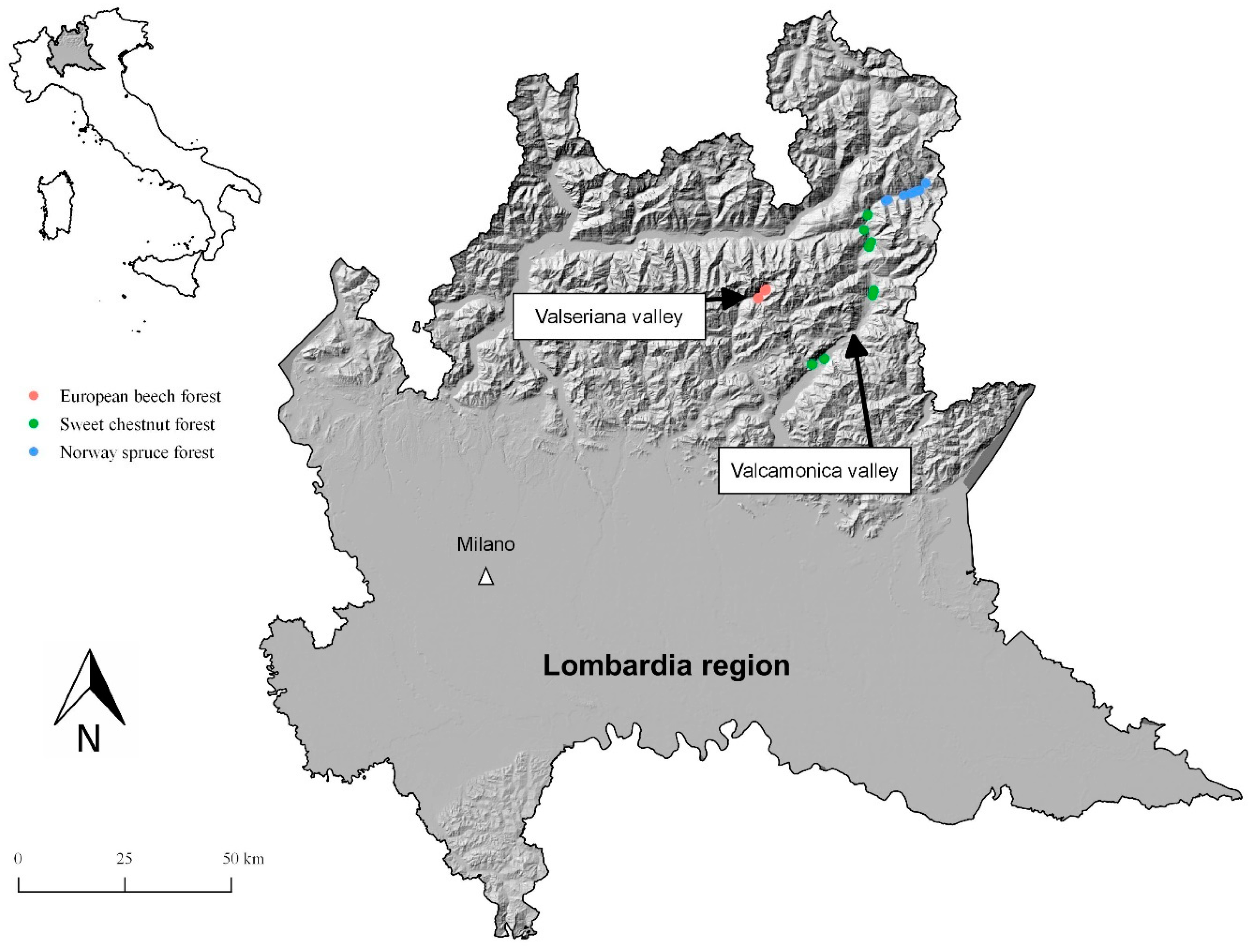
2.1. Study Area

The study area is located in northern Valcamonica and in northern Valseriana, two alpine valleys of the Lombardia region, in the southeastern Italian Alps (Figure 1). The climate of the Valcamonica is Cfb (cold, without dry season, and with warm summer) while the climate of the Valseriana is Dfb (temperate, without dry season, and with warm summer) [23]. The geological substrate of these two valleys is strongly heterogeneous and it is composed by different types of rock, such as volcanic (granite, tonalite, gabbro, and diorite; especially in the Adamello mountains) and sedimentary rocks (dolomite, conglomerate, and sandstone; especially in the Orobic Prealps and in lowest zones of the valleys). The morphology of these two valleys was shaped during the Würm glaciation (the last glacial period of the Alpine region, 100,000–10,000 years ago) when the alpine glaciers expanded all the way up to the Po Plain. In the study domain, the highest peaks are Mount Adamello (Adamello Alps; 3554 m asl) and Mount Cima di Caronno (Orobic Alps; 2945 m asl). Oglio river flows along Valcamonica, from Ponte di Legno to Iseo lake. Serio river rising from the Mount Torena (upper Valseriana, 2911 m asl) runs across Valseriana. Most of the study area is covered by large forests: in Valcamonica the dominant forest types are sweet chestnut forest and Norway spruce forest, while in northern Valseriana, European beech forest.

2.2. Sampling Sites and Data Collection

In the first stage of the study, different cartographic layers of the study area were collected. From a regional map of forest types, three forest types were selected: European beech forest, sweet chestnut forest, and Norway spruce forest. Forest management plans were used to distinguish public from private forest property. Only public forest areas with a suitable accessibility were included in the study. Within this domain, 50 sampling plots (1256 m² surface) were randomly distributed: 10 plots in European beech forest, 20 plots in sweet chestnut forest, and 20 plots in Norway spruce forest (Figure 1). Sampling was performed from May to October 2019. All living trees (if DBH [diameter at breast height] > 7.5 cm), inside each plot, were measured for: position (x and y coordinates), DBH, and total height.

2.3. Stand Structural Indices

In the following sections we provide a brief review of the eight stand structural indices used in this study: the Gini index, the Shannon index, the R aggregation index, the Diameter dominance index, the Diameter differentiation index, the Mingling index, the Tree height dominance index, and the Tree height differentiation index.

2.3.1. Gini Index

The Gini index (G) was introduced by the Italian statistician Corrado Gini [24]. Derived from the Lorentz curve [25], it is one of the most common measures of national income inequality [26]. The Gini index can be used to assess the size variation within a forest stand as a spatially inexplicit index of forest structure [27]. The DBH of all sampled trees is measured and collected into a dataset, then sorted in ascending order. From each DBH, the basal area is calculated. Then, the proportions of cumulative basal area per hectare and the proportions of the cumulative number of trees per hectare are defined. Plotting these two series of values on the y and x axis, respectively, gets the Lorentz curve. Once plotted the curve, two areas come to be formed: the area between the Lorentz curve and the 45° line, and the total area under the 45° line. The Gini index is the ratio of these two areas [15] and ranges between 0 and 1. The more the index is near 1, the more heterogeneous distribution the stem basal area has. Conversely, if the index assumes values near to 0, trees have or are near to have the same size; therefore, the differentiation is low [28].

2.3.2. Shannon Index

The Shannon index (H) is one of the most used indices for assessing species diversity and it is considered a good indicator of both dominance and richness of species [29]. It is even known as Shannon–Wiener index [30]. The formula is the following:

$$H=-{\displaystyle \sum }_{i=1}^n{p}_{i}ln\left(p_i\right)$$

(1)

where, p_i is the proportion of individuals belonging to i-th species on the total number of the individuals in the sampling unit [31]. H ranges between 0 and (theoretically) infinity [32]. When the index tends to 0, the individuals are mainly concentrated into one species; thus, the species diversity is very low.

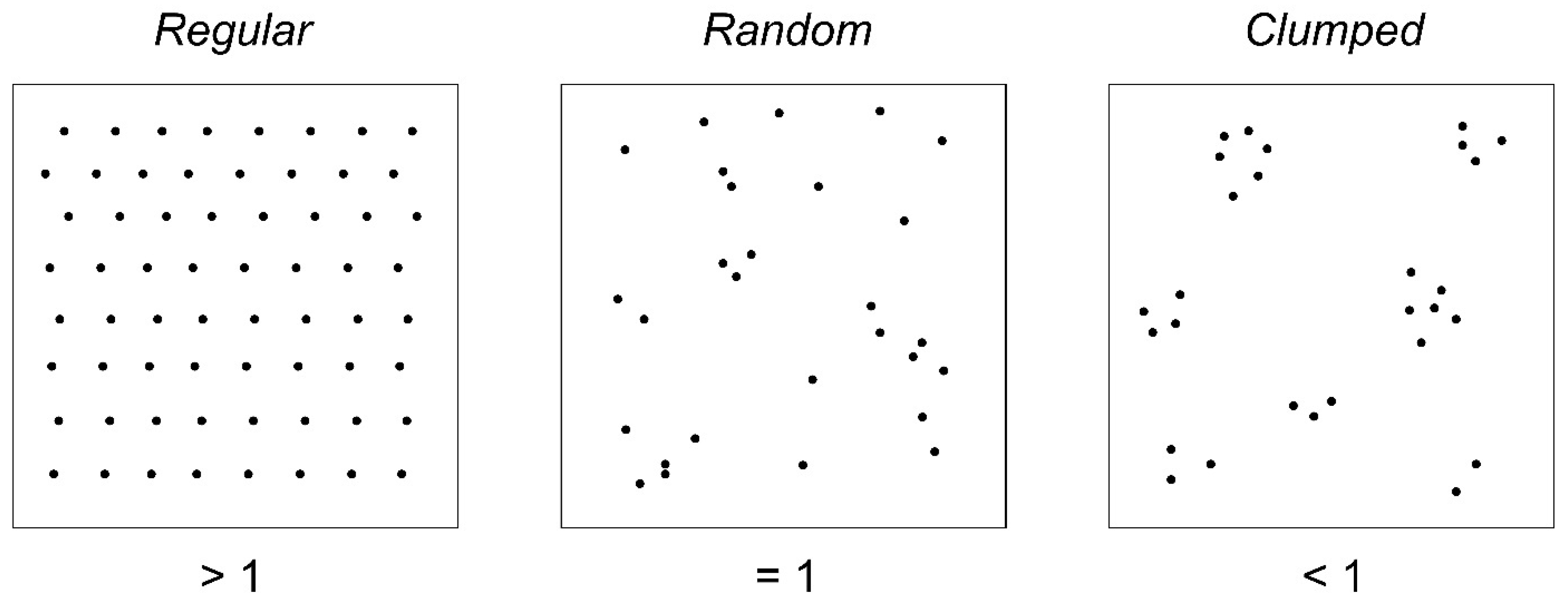
2.3.3. R Aggregation Index

The R aggregation index (R) is a measure of location diversity in non-marked point patterns [16]. This index was formulated by Philip J. Clark and Francis C. Evans [33] and is given by the ratio:

$$R=\frac{r_A}{r_E}$$

(2)

where, r_A is the mean of the distance between each point of the point pattern and its nearest neighbor, and r_E is the mean distance in a reference large random distribution. The large random distribution characteristics are expressed by the ratio between the number of individuals observed in the studied population (N) and the sampled area (A) [16,33,34]. The formula for r_E is the following:

$$r_E=\frac{1}{2\sqrt{\frac{N}{A}}}$$

(3)

The R aggregation index ranges between 0 and 2.149, the maximum value it can assume. If it is =1, the population has random spatial distribution. If it is >1, the population tends to regular pattern. If it is <1, the population tends to be clumped (or clustered) [12,35]. Figure 2 shows three possible configurations of forest population in function of R aggregation index.

2.3.4. Diameter Dominance Index

The Diameter dominance index (U) is an index of size dominance and is computed from a point pattern marked with quantitative marks [16]. In this case, the quantitative mark is the DBH. Starting from a reference tree, i, if its DBH exceeds the DBH of the nearest neighbor j, the function turns 1; conversely 0. This binary problem is turned for each of the k nearest neighbors of i. Commonly, the 4 nearest neighbors of i are used (k = 4). The mean of the 4 obtained values is the dominance index of the reference tree (U_i) according to the equation:

$$U_i=\frac{1}{k}{\displaystyle \sum }_{j=1}^{k}1(DB{H}_i>DB{H}_j)$$

(4)

The U_i is computed for each tree of the population and can assume 5 discrete values (k + 1): 0.00 (the i tree is very suppressed), 0.25 (the i tree is moderately suppressed), 0.5 (the i tree is co-dominant), 0.75 (the i tree is dominant), 1.00 (the i tree is strongly dominant). It is possible to calculate the population mean as the mean of all the U_i values obtained in the sampled population [16,36].

2.3.5. Diameter Differentiation Index

The Diameter differentiation index (T) is a size diversity index. The DBH (mark) of the reference tree (DBH_i) is compared to the diameter of each of its k nearest neighbors (DBH_j) [13]. The mean of the ratio between the smaller and the larger diameter of each comparison is then subtracted from 1, according to the following equation:

$$T_i=1-\frac{1}{k}{\displaystyle \sum }_{j=1}^k\frac{\min \left(DB{H}_i,DB{H}_j\right)}{\max \left(DB{H}_i,DB{H}_j\right)}$$

(5)

The specific use with the DBH is operated in this study, while originally the index was proposed as a size differentiation index where the DBH, as in the above-reported equation, could be replaced with other types of quantitative marks, such as tree height, tree volume, tree biomass, and tree growth rate or volume increments. When T_i is equal to 0, the reference tree and its neighbors have the equal diameter size. Conversely, when the T_i tends to its theoretical maximum (=1), the diameter differentiation is the highest [16]. According to Pommerening and Grabarnik [16], the index values can be grouped in four ranges. When 0 < T_i ≤ 0.3, smaller tree has at least the 70% of the neighbor tree’s diameter; when 0.3 < T_i ≤ 0.5, smaller tree has 50–70% of the neighbor tree’s diameter; when 0.5 < T_i ≤ 0.7, smaller tree has 30–50% of the neighbor tree’s diameter; when 0.7 < T_i ≤ 1, smaller tree has less than 30% of the neighbor tree’s diameter. By analogy with the Diameter dominance index, it is possible to calculate the population mean as the mean of all the T_i values obtained in the sampled population.

2.3.6. Mingling Index

Very similar to the Diameter dominance index is the Mingling index (M) that could be described as an extension to the nearest neighbor analysis of the Pielou’s segregation coefficient [37]. However, the Mingling index belongs to the group of the species diversity indices and its computation is based on a point pattern marked with the tree species as qualitative mark. The equation for the Mingling index is the following:

$$M_i=\frac{1}{k}{\displaystyle \sum }_{j=1}^{k}1\left(m_i\ne m_j\right)$$

(6)

By analogy with the Diameter dominance index, each comparison between the reference tree and its k nearest neighbors is turned into a binary problem. If the species of the reference tree (i) is equal to the species of the nearest neighbor tree (j), the result of the comparison will be 0; conversely, the result will be 1. The arithmetic mean of all the comparison gives the M_i for a reference tree. The index ranges from 0 to 1: when it is 1, the mingling is maximum; conversely, when the index is 0, the reference tree and its nearest neighbors belong to the same species [12,13]. Again, it is possible to calculate the population mean as the mean of all the M_i values obtained in the sampled population.

2.3.7. Tree Height Dominance and Differentiation Indices

The same principles of size dominance and differentiation used in the Diameter dominance index and in the Diameter differentiation index are used to calculate the Tree height dominance index (Uh) and the Tree height differentiation index (Th). The equations are the same described in Section 2.3.4 and Section 2.3.5, except that the mark of each point was defined as the tree total height rather than the DBH.

2.3.8. Indices Means and Edge Correction

In this study, for each sampling plot we obtained a mean (population mean) of each stand structural index. However, the population means may suffer the edge effect, also known as edge bias. To overcome this problem, we used the NN1 edge correction for the calculation of the Diameter dominance and differentiation indices, the Mingling index, the Tree height dominance and differentiation indices, whereas, for the R aggregation index, we used the Cumulative Distribution Function method (cdf), which is based on the Kaplan–Meier edge correction [38]. G and H bypassed the edge correction as they are spatially inexplicit indices, and their results are already in form of a mean value for each sampling plot.

2.4. Stand Structural Parameters

In addition to the above-mentioned stand structural indices, five common stand structural parameters were calculated: The Number of trees (N), the Basal area per hectare (B), the Mean diameter (d), the Dominant height (Dh), and the Stand volume per hectare (V). The Number of trees per hectare is the total number of trees found in each sampling plot recalculated per hectare. The Basal area per hectare was calculated comparing the basal area of each sampling plot to the surface of one hectare. The basal area of a sampling plot was the sum of the basal areas of each tree, obtained applying the well-known and common equation based on the formula for the area of a circle to each DBH. The Mean diameter was calculated from the mean basal area using the inverse of the formula for the area of a circle. The Dominant height (even known as Top height) is defined as the average height of a fixed number of trees in a stand that present the largest DBH. Usually, for one hectare, the 100 largest trees are used. In this study, considering that the sampling plots had a surface of 0.125 hectare and applying a proportion to 100 trees per one hectare, the 12 largest trees in each sampling plot were used to obtain the Dominant height. The Dominant height is a good indicator for the site productivity, and it is preferred to the mean height because it is not influenced by the stand density [39]. The Stand volume per hectare was calculated comparing the stand volume of each sampling plot to the surface of one hectare. The stand volume of the sampling plot was the sum of the volume of each tree in the plot, that was calculated through the equations provided by Tabacchi et al. [40], starting from its DBH and total height.

2.5. Software Processing and Statistics

All the stand structural indices and the statistics were performed using the R software (v. 3.6.1) [41]. For the Gini index, the function gini was used, from the reldist library (version 1.6–6) [42,43]. For the Shannon index, the function diversity was used, from the vegan library (version 2.5–7) [44]. The R aggregation index was calculated with the clarkevans.test function, from the spatstat library (2.3–0) [45,46]. The remaining stand structural indices were calculated with the R scripts present in Pommerening and Grabarnik [16]. All the spatially explicit stand structural indices were calculated using four nearest neighbors per reference tree (k = 4). The R code for the NN1 edge correction was retrieved from Pommerening and Grabarnik [16]. The Cumulative Distribution Function edge correction, used for the R aggregation index, was included in the clarkevans.test function. The stand structural indices were checked for normality and homoscedasticity requirements using the Shapiro–Wilk test (p > 0.05) and Levene’s test (p < 0.05), respectively. Since some indices showed non-normal frequency distributions or heteroscedasticity, statistical differences, of each structural index, among forest types were tested using the non-parametric Kruskal–Wallis test (p < 0.05). Levene’s test was also used to evidence differences of the distribution of each index in function of the forest type (p < 0.05). Then, a principal component analysis (PCA) and the non-parametric Spearman’s rank correlation test were carried out to examine the correlations among the stand structural indices. Spearman’s rank correlation coefficient was also used for assessing the correlations between stand structural indices and stand structural parameters, both for each forest type and for the aggregated dataset.

3. Results

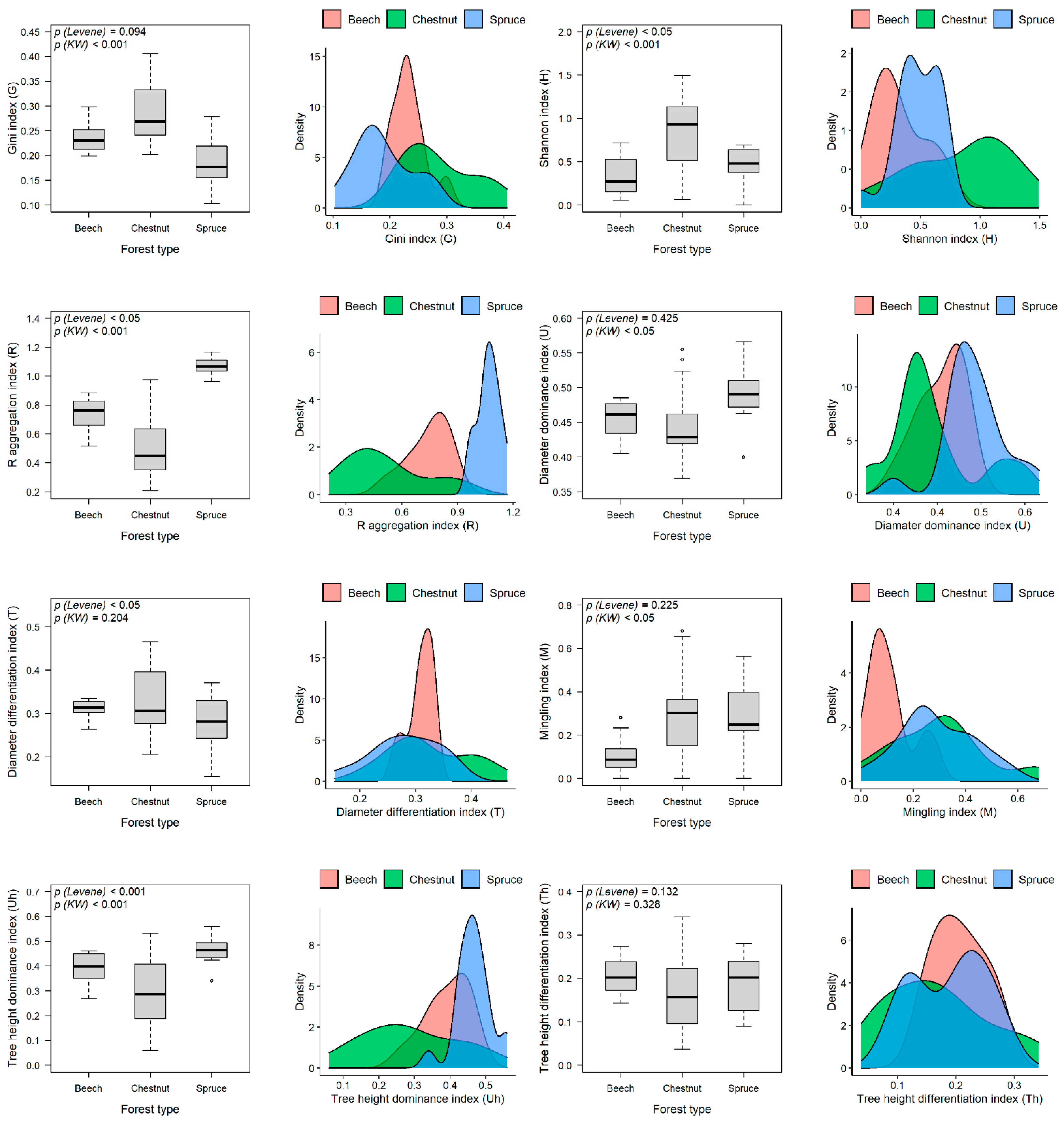
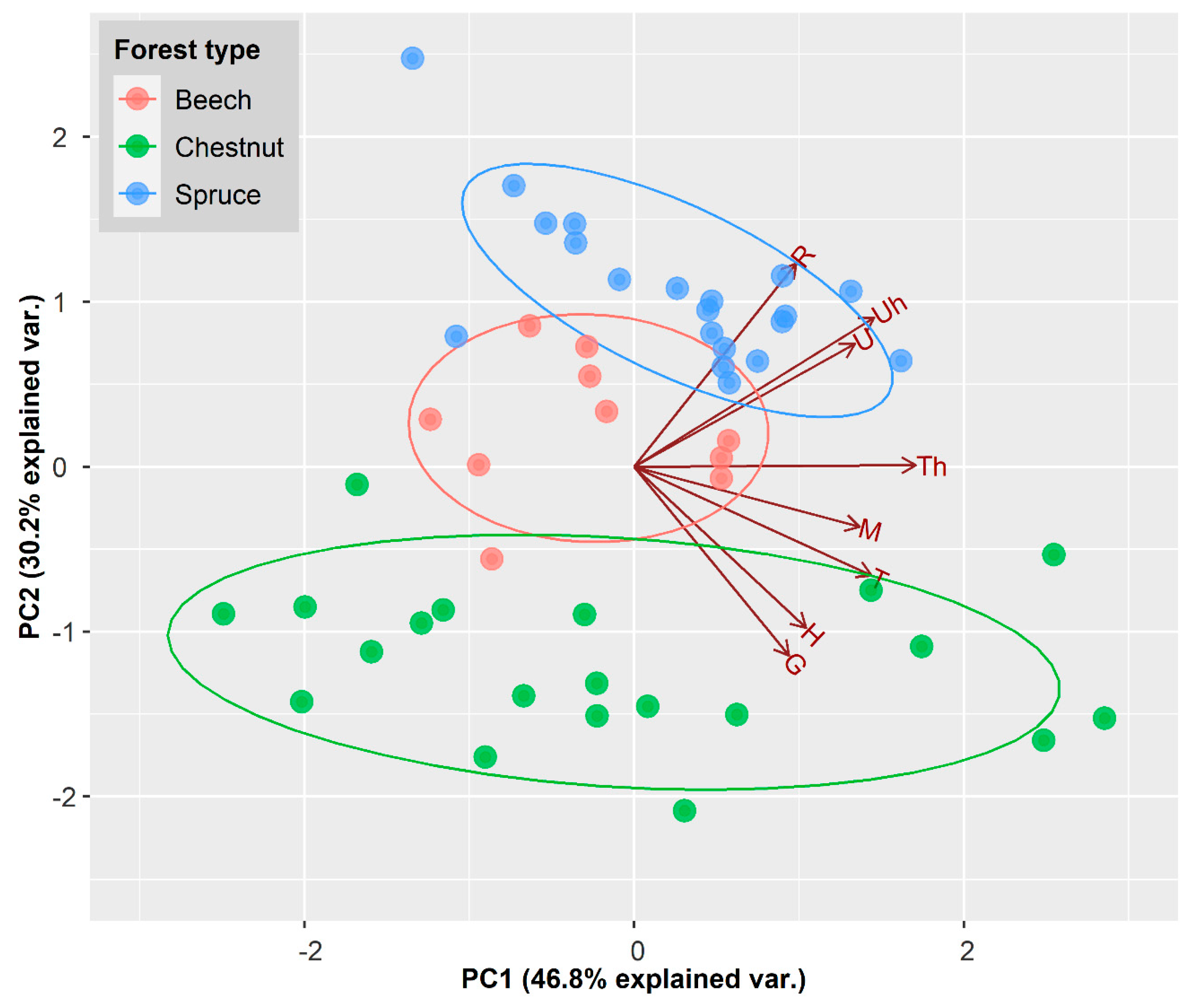
3.1. Stand Structural Indices across Forest Types

Almost all the analyzed stand structural indices statistically varied among forest types according to the Kruskal–Wallis test (Figure 3). G (p < 0.001), S (p < 0.001), R (p < 0.001), U (p < 0.05), M (p < 0.05), and Uh (p < 0.001) were statistically different among forest types, whereas T (p = 0.204) and Th (p = 0.328) excluded any statistical differences among spruce, chestnut, and beech forests. Strong differences have been found in G, H, R, and Uh, where p < 0.001. The highest G was showed by chestnut forest (0.29 ± 0.30), followed by spruce forest (0.19 ± 0.05), and beech forest (0.23 ± 0.61). The same pattern was showed by H: chestnut forest (0.84 ± 0.40), spruce forest (0.48 ± 0.17), and beech forest (0.33 ± 0.21). The highest R was found in spruce forest (1.07 ± 0.06), followed by beech (0.74 ± 0.11) and chestnut (0.52 ± 0.21). The highest Uh was found in spruce (0.47 ± 0.05), while the lowest was found in chestnut (0.29 ± 0.13). The distributions of variances varied among forest types according to Levene’s test. For example, R (p < 0.05) and Uh (p < 0.001) showed a noticeable concentration of values around the mean in spruce forest, whereas in beech and in chestnut forest, especially, the values were more widely distributed. This last evidence revealed a higher variability of stand structure configurations within the forest type. Conversely, in G (p = 0.094), U (p = 0.425), M (p = 0.225), and Th (p = 0.132), the variances resulted as homogeneously distributed among forest types.

The PCA biplot shows a synthesis of the previous described results (Figure 4). The first Principal Component (PC) explains almost the half of variance (46.8%) and the second PC more than 30%. The distribution of the samples reveals a marked subdivision reading the graph from the top with the spruce samples to the bottom with the chestnut samples, and the beech samples in the middle. Spruce forest shows higher values of R, and of U and Uh. Conversely, the chestnut samples revealed a moderate accordance with higher values of G and H. The cluster of beech forest are located as an intermediate group with no marked stand characteristics. Graphically, Th seems to be not influenced by the forest types.

3.2. Correlation among Stand Structural Indices

The correlation among stand structural indices gave different results in function of the forest type, as expected. In beech forest, the Spearman test gave six significant correlations between stand structural indices. In four of them, the correlation coefficient (r) was greater than 0.7. G was positively correlated with H (p < 0.001; r = 0.709); R was positively correlated with U (p = 0.009; r = 0.806) and Uh (p = 0.001; r = 0.758), and the highest correlation coefficient (p = 0.001; r = 0.891) was found between H and M. The chestnut forest gave the highest results in terms of number of significant correlations. Twenty-seven comparisons were statistically significant, fourteen of them were greater than 0.7, evidencing strong positive associations. The highest correlations were found between G and Th (p < 0.001; r = 0.830); H and M (p < 0.001; r = 0.911); T and Uh (p < 0.001; r = 0.848); M and Uh (p < 0.001; r = 0.889); T and Th (p < 0.001; r = 0.845); M and Th (p < 0.001; r = 0.839); the two Tree height indices between each other (p < 0.001; r = 0.970). In spruce forest, four comparisons provided r values greater than 0.7. The highest correlation coefficients were found between the G and T (p < 0.001; r = 0.832); T and Th (p < 0.001; r = 0.899); H and M (p < 0.001; r = 0.892). When the correlation is computed on the whole of the sampling plots, only four correlations gave r greater than 0.7. Among them, the highest correlation coefficient was found between H and M (p < 0.001; r = 0.842) (

Table 1. Correlation coefficients (Spearman’s r) between stand structural indices and stand structural parameters in the European beech forest. Associations that were statistically significant (p < 0.05) are in bold.

	1	2	3	4	5	6	7	8	9	10	11	12	13
1. Gini index (G)	1.000
2. Shannon index (H)	0.709	1.000
3. R aggregation index (R)	0.382	0.430	1.000
4. Diameter dominance index (U)	0.394	0.321	0.806	1.000
5. Diameter differentiation index (T)	0.515	0.467	0.467	0.600	1.000
6. Mingling index (M)	0.636	0.891	0.309	0.358	0.721	1.000
7. Tree height dominance index (Uh)	0.164	0.152	0.758	0.624	0.139	−0.030	1.000
8. Tree height differentiation index (Th)	0.515	0.418	0.600	0.527	0.624	0.418	0.673	1.000
9. Number of trees (N)	0.018	0.442	−0.188	−0.273	−0.079	0.491	−0.442	−0.394	1.000
10. Basal area per hectare (B)	0.122	0.632	0.182	0.024	−0.049	0.517	−0.164	−0.328	0.833	1.000
11. Mean diameter (d)	0.127	0.067	0.406	0.212	−0.176	−0.224	0.152	−0.236	−0.224	0.249	1.000
12. Tree dominant height (Dh)	0.377	0.840	0.340	0.204	0.321	0.735	0.241	0.253	0.488	0.690	0.056	1.000
13. Stand volume (V)	0.103	0.636	0.152	0.006	−0.030	0.539	−0.188	−0.321	0.855	0.997	0.200	0.704	1.000

,

Table 2. Correlation coefficients (Spearman’s r) between stand structural indices and stand structural parameters in the sweet chestnut forest. Associations that were statistically significant (p < 0.05) are in bold.

	1	2	3	4	5	6	7	8	9	10	11	12	13
1. Gini index (G)	1.000
2. Shannon index (H)	0.696	1.000
3. R aggregation index (R)	0.636	0.538	1.000
4. Diameter dominance index (U)	0.495	0.374	0.695	1.000
5. Diameter differentiation index (T)	0.744	0.516	0.746	0.765	1.000
6. Mingling index (M)	0.725	0.911	0.672	0.642	0.719	1.000
7. Tree height dominance index (Uh)	0.789	0.782	0.761	0.606	0.848	0.889	1.000
8. Tree height differentiation index (Th)	0.830	0.752	0.798	0.586	0.845	0.839	0.970	1.000
9. Number of trees (N)	−0.696	−0.550	−0.649	−0.457	−0.797	−0.642	−0.851	−0.810	1.000
10. Basal area per hectare (B)	−0.002	−0.312	0.349	0.176	0.204	−0.099	−0.020	0.037	0.030	1.000
11. Mean diameter (d)	0.648	0.337	0.767	0.549	0.777	0.526	0.738	0.746	−0.847	0.441	1.000
12. Tree dominant height (Dh)	0.248	0.116	0.440	0.275	0.286	0.253	0.329	0.301	−0.472	0.482	0.709	1.000
13. Stand volume (V)	0.101	−0.206	0.394	0.192	0.230	−0.002	0.087	0.120	−0.135	0.929	0.582	0.744	1.000

,

Table 3. Correlation coefficients (Spearman’s r) between stand structural indices and stand structural parameters in the Norway spruce forest. Associations that were statistically significant (p < 0.05) are in bold.

	1	2	3	4	5	6	7	8	9	10	11	12	13
1. Gini index (G)	1.000
2. Shannon index (H)	−0.080	1.000
3. R aggregation index (R)	0.250	−0.072	1.000
4. Diameter dominance index (U)	0.220	−0.041	−0.153	1.000
5. Diameter differentiation index (T)	0.832	0.150	0.129	0.208	1.000
6. Mingling index (M)	−0.259	0.892	−0.066	−0.092	0.006	1.000
7. Tree height dominance index (Uh)	0.287	0.208	−0.129	0.205	0.417	0.299	1.000
8. Tree height differentiation index (Th)	0.741	0.075	−0.045	0.158	0.899	0.009	0.495	1.000
9. Number of trees (N)	0.115	0.183	0.084	−0.159	0.074	−0.014	−0.139	0.026	1.000
10. Basal area per hectare (B)	0.100	0.322	0.196	−0.181	0.140	0.248	−0.111	−0.056	0.396	1.000
11. Mean diameter (d)	−0.158	−0.153	−0.044	0.167	−0.069	0.054	0.000	−0.087	−0.890	−0.096	1.000
12. Tree dominant height (Dh)	0.286	−0.015	0.256	0.364	0.290	0.011	0.288	0.188	−0.621	−0.017	0.697	1.000
13. Stand volume (V)	0.074	0.051	0.286	0.000	0.186	0.044	0.170	0.020	0.177	0.689	0.060	0.318	1.000

and

Table 4. Correlation coefficients (Spearman’s r) between stand structural indices and stand structural parameters in the whole of the sampling plots. Associations that were statistically significant (p < 0.05) are in bold.

	1	2	3	4	5	6	7	8	9	10	11	12	13
1. Gini index (G)	1.000
2. Shannon index (H)	0.477	1.000
3. R aggregation index (R)	−0.403	−0.161	1.000
4. Diameter dominance index (U)	−0.038	0.024	0.649	1.000
5. Diameter differentiation index (T)	0.688	0.317	0.022	0.314	1.000
6. Mingling index (M)	0.182	0.842	0.214	0.300	0.307	1.000
7. Tree height dominance index (Uh)	−0.150	0.076	0.756	0.761	0.253	0.387	1.000
8. Tree height differentiation index (Th)	0.432	0.284	0.347	0.508	0.772	0.381	0.649	1.000
9. Number of trees (N)	0.055	−0.205	−0.549	−0.539	−0.196	−0.470	−0.602	−0.357	1.000
10. Basal area per hectare (B)	−0.391	−0.121	0.579	0.283	−0.059	0.161	0.302	−0.031	−0.200	1.000
11. Mean diameter (d)	−0.214	0.076	0.695	0.591	0.120	0.417	0.604	0.250	−0.877	0.591	1.000
12. Tree dominant height (Dh)	−0.436	−0.171	0.825	0.598	−0.060	0.173	0.688	0.222	−0.542	0.665	0.757	1.000
13. Stand volume (V)	−0.218	−0.094	0.460	0.297	0.088	0.104	0.291	0.035	−0.173	0.863	0.533	0.634	1.000

).

3.3. Correlation between Stand Structural Indices and Stand Structural Parameters

Spruce stands excluded any statistically significant correlations between stand structural indices and stand structural parameters (p > 0.05). On the other hand, in beech stands, significant positive correlations were found between the Dh and both the two indices of species diversity (H: p < 0.05, r = 0.840; M: p < 0.05, r = 0.735). Significant associations were also found in chestnut stands, where seven comparisons gave r values major than 0.7. Negative correlations were found between N and both Uh and Th (p < 0.001; r < −0.800). Moreover, a high positive correlation was found between the d and R (p < 0.001; r = 0.767). T resulted as positively correlated with d (p < 0.001; r = 0.777) and negatively correlated with N (p < 0.001; r = −0.797). When the whole of the sampling plots was used in the correlation test, only the association between Dh and R provided a correlation score greater than 0.7 (p < 0.001; r = 0.825) (Table 1, Table 2, Table 3 and Table 4).

4. Discussion

4.1. Stand Structural Indices across the Analyzed Forest Types

The results of this study clearly indicate that the stand structural indices vary among forest types. The Gini index, the Shannon index, the R aggregation index, the Diameter dominance index, the Mingling index, and the Tree height dominance index were statistically different among the three analyzed forest types (p < 0.05). The highest variability within each stand structural index was showed by the chestnut forest. This result could be associated to the high structural and silvicultural variability found in the chestnut stands. Chestnut sampling plots are representative of different forest management systems including coppice, high forest, and other intermediate systems (Figure 5a,b). Since the mid-1900s, most of the chestnut stands have been cultivated as orchards, with a low density (usually, from 50 to 80 individual per hectare) of tall and big trees. In recent years, the depopulation of mountain villages and the use of alternative food sources caused an inexorable abandonment of the chestnut orchards. Many of them are now managed as coppice for timber production, some are the result of a mixture between coppice and high forest management, some others are uncultivated, favoring an increase of complexity in stand structure and species composition. The increasing structural and species composition complexity is underlined by the results obtained in the Gini index, the Shannon index, and the Mingling index, where chestnut forest shows the highest mean values as well as the largest variation. On the other hand, chestnut forest reveals lower values of the R aggregation index than beech and spruce forest. Spruce forest showed average R aggregation index larger than 1, typically representative of a regular spatial distribution. This type of distribution has been for centuries artificially generated and favored by management practices in the Alps, as confirmed by the fact that original mixed compositions and irregular structures can be restored in areas untouched for some decades [47]. Most of these planted stands have been changing their structure, but, in some cases, the results from the R aggregation index reveal the original reforestation design with a grid pattern and uniform distances among trees (Figure 5c). On the other hand, despite the presence of a high variability, in chestnut stands, a low average value of the R aggregation index reveals the presence of clumped pattern typical of coppice management, as already suggested by some research works [15,48,49]. The distribution of the R aggregation index in beech forest reveals the presence of near-to random spatial distributions. This pattern is in accordance with the current management undertaken in beech stands of the Valseriana valley. Here, beech forest has usually been managed as coppice for firewood. However, forest managers now prefer to convert the coppice system to even-aged high forest, which are considered more productive [50]. The conversion of coppice into high forest is carried out through thinning aimed to reduce to one the sprouts of each stump (Figure 5d). Thinning strongly influences the spatial distribution of trees [51]; in fact, random distributions have been also found after heavy thinning in Scots pine stands by Crecente-Campo et al. [52]. Average Diameter dominance index ranged between 0.4 and 0.5 in all the forest types, revealing a high frequency of co-dominant trees. The general low size differentiation found in beech and spruce may be linked to thinning. It has been shown that thinning, and especially thinning from below, can lead to low diameter differentiation [51]. Moreover, regular plantation and semi-natural stands can show different values of the size differentiation indices, with a general higher differentiation in the latter [53]. The PCA reveals that the combined use of several stand structural indices can strongly support to distinguish forest types from each other. Forest types were clearly separated along the second axis that displayed the heterogeneity of the stand structural indices. The results obtained demonstrate that there are grounds for an automatic identification of the forest types based on their stand structure that is feasible with a combination of multiple structural indices analyzed through appropriate statistical techniques. To date, there are only a few studies that have conducted similar analysis, even with results in line with those presented in this article [22,54]. Schall et al. [22] distinguished even-aged beech forests from pine and immature/mature spruce forests using a PCA and a set of stand structural attributes. The classification of forest types based on their structural features seems be promising, but further studies on this topic are needed. In this context, the use of three-dimensional data from Lidar technology [55,56] can provide a way to easily and quickly detect the relative position and the dimension of forest trees.

4.2. Relationship between Stand Structural Indices and Stand Structural Parameters

The correlation among stand structural indices indicates that some of them are strongly correlated between each other and, thus, they can give redundant information. Namely, the Shannon index and the Mingling index, both species diversity indices, were strongly correlated in each forest type. The advantage of the choice of the Shannon index rather than the Mingling index is to reduce cost and time of surveys since the Shannon index does not require the position of the trees for its computation. The association between spatially explicit and inexplicit structural indices was also explored by Sterba [15]. He compared the Shannon index and the Pielou’s Index of Segregation (spatially explicit) as indices of species diversity, with non-significant results. On the other hand, a strong positive correlation between the Shannon and the Mingling indices was also found by Keren et al. [21] and by Schall et al. [22]. In our study, significant associations were found between the Gini index and the Diameter differentiation index, both indices of diameter differentiation. The results only partially reflect the expectations since the significant correlation was only found in chestnut and spruce forests. A significant correlation was also obtained testing the whole of the sampling plots, even if the correlation coefficient was lower than 0.7 (r = 0.688). The highest correlation coefficient, found in spruce, is probably linked to the even-aged structure of the stands. Indeed, strong significative and positive correlations between the Gini index and the Diameter differentiation index have often been found in even-aged forests [21,57]. In other cases, the correlation was, even if significant, only barely so [15,21]. Moreover, in our analysis, strong correlations have been found between the spatially explicit size dominance indices. Namely, the Diameter dominance index was correlated with the Tree height dominance index, while the Diameter differentiation index was correlated with the Tree height differentiation index. The association is due to the non-linear relation that exists between DBH and height [22]. The results indicate that there is no need to collect both DBH and tree height during filed surveys when the aim is studying size dominance or differentiation.

The most evident correlations between stand structural indices and stand structural parameters are those recorded in the chestnut forest between the number of trees and both the size differentiation indices. The results indicate that the higher the number of trees, the lower the differentiation. When the whole of the forest types is analyzed, a strong correlation is found between the Dominant height and the R aggregation index, indicating that the highest tree heights are found when the spatial distribution of trees moves toward random or regular patterns. The correlation between the Gini index and the Mean diameter have already been reported in other works with opposite results. Namely, Schall et al. [22] found a negative correlation between Gini index and Mean diameter, whereas Keren et al. [21] reports moderately strong positive correlation on plots of 1000 m² and 1500 m². However, from our results, we can only remark a significant but weak positive correlation limited to the chestnut forest.

4.3. Limitation of the Study, Recommendations, and Suggestions for Future Research

In this study, the stand structural indices represent population means, namely, plot means. As revealed in the scientific literature, the population means of the spatially explicit indices may suffer the edge effect [16]. For this reason, edge correction is an inevitable step in calculating the stand structural indices. In this study, we used the NN1 edge correction, which belongs to the group of the minus-sampling edge corrections. It has been shown that for very small circular plots, minus-sampling edge corrections may not be performing methods for the edge bias mitigation, causing appreciable variance. Conversely, the plus-sampling technique seems to be more robust and reliable edge-correction method [58,59]. However, Barbeito et al. [18] found that a plot size of 1000–2000 m² is sufficient for obtaining accurate and unbiased results from the application of population means. Moreover, NN1 edge correction is a secure estimator when the sample is composed by a sufficiently large number of trees [60]. However, when the sampling units are small circular sampling plots, like those commonly used in forest inventories (500–600 m²), other edge corrections are preferable, such as the plus-sampling or the recently tested spatial forest reconstruction [16,58].

During the computation of the spatially explicit stand structural indices, we used a fixed number of four nearest neighbors. However, it would be better to calculate the indices using a variable number of neighbors and test their differences. Indeed, according to Keren et al. [21], the indices calculated with four neighbors were higher than those calculated with a lower number of neighbors.

An evident limitation of the present study deals with the number of the sampling units. Ten to twenty sampling plots may be barely sufficient to infer on the whole of a forest type in large study areas. However, we are still far from a clear understanding of how many sampling units are needed in function of the study area extension.

Another important limitation regards the structural variability of the analyzed sample. The results from the Gini index, which never exceeded 0.5, indicate that, even if with a considerable variability, the forest stands investigated in this article are even-aged [48,61]. Forest samples with small range of structural variability increase the chance of correlation between stand structural indicators. In line with the last two mentioned limitations, a recommendation for future research studies is to use larger sample sizes and a higher number of sampling units per forest type. Moreover, the samples should cover the entire structural variability present in the area under study.

5. Conclusions

The results indicate that the stand structural indices vary among the analyzed forest types. The PCA revealed that the combined use of several stand structural indices helps to distinguish forest types from each other. The correlation among stand structural indices indicates that some of them are strongly intercorrelated and, thus, they can give redundant information. Strong correlations have been found between spatially explicit and inexplicit indices. Namely, between the Shannon index and the Mingling index, and between the Gini index and the Diameter differentiation index. Furthermore, strong correlations have been found between the spatially explicit size dominance indices: the Diameter dominance index was correlated with the Tree height dominance index, whereas the Diameter differentiation index was correlated with the Tree height differentiation index. Correlations between stand structural indices and stand structural parameters were recorded between the number of trees and both the size differentiation indices (in chestnut forest), between the Dominant height and the R aggregation index. Regarding the correlation between the Gini index and Mean diameter, we report a significant but weak positive correlation limited to the chestnut forest. However, due to the general scarcity of correlations obtained, we cannot recommend the exclusive use of stand structural indices as alternative to the common stand structural parameters. It is instead advised to use a combination of stand structural indices and parameters. In line with the limitations raised during the interpretation of results, we recommend future research studies to explore more forest types, using larger sample sizes and higher number of sampling units per forest type. Moreover, the samples should cover the entire structural variability present in the study area, avoiding selecting only even-aged or uneven-aged stands.

References

1. Bagnaresi, U.; Giannini, R.; Grassi, G.; Minotta, G.; Paffetti, D.; Pini Prato, E.; Proietti Placidi, A.M. Stand structure and biodiversity in mixed, uneven-aged coniferous forests in the eastern Alps. Forestry 2002, 75, 357–364. [Google Scholar] [CrossRef] [Green Version]
2. Touihri, M.; Villard, M.A.; Charfi, F. Cavity-nesting birds show threshold responses to stand structure in native oak forests of northwestern Tunisia. For. Ecol. Manag. 2014, 325, 1–7. [Google Scholar] [CrossRef]
3. Joelsson, K.; Hjältén, J.; Work, T. Uneven-aged silviculture can enhance within stand heterogeneity and beetle diversity. J. Environ. Manag. 2018, 205, 1–8. [Google Scholar] [CrossRef]
4. Gao, T.; Hedblom, M.; Emilsson, T.; Nielsen, A.B. The role of forest stand structure as biodiversity indicator. For. Ecol. Manag. 2014, 330, 82–93. [Google Scholar] [CrossRef]
5. Dănescu, A.; Albrecht, A.T.; Bauhus, J. Structural diversity promotes productivity of mixed, uneven-aged forests in southwestern Germany. Oecologia 2016, 182, 319–333. [Google Scholar] [CrossRef]
6. Zhang, Y.; Chen, H.Y.H. Individual size inequality links forest diversity and above-ground biomass. J. Ecol. 2015, 103, 1245–1252. [Google Scholar] [CrossRef]
7. Ali, A. Forest stand structure and functioning: Current knowledge and future challenges. Ecol. Indic. 2019, 98, 665–677. [Google Scholar] [CrossRef]
8. Ali, A.; Lin, S.L.; He, J.K.; Kong, F.M.; Yu, J.H.; Jiang, H.S. Climate and soils determine aboveground biomass indirectly via species diversity and stand structural complexity in tropical forests. For. Ecol. Manag. 2019, 432, 823–831. [Google Scholar] [CrossRef]
9. Vieira, J.; Matos, P.; Mexia, T.; Silva, P.; Lopes, N.; Freitas, C.; Correia, O.; Santos-Reis, M.; Branquinho, C.; Pinho, P. Green spaces are not all the same for the provision of air purification and climate regulation services: The case of urban parks. Environ. Res. 2018, 160, 306–313. [Google Scholar] [CrossRef]
10. Cislaghi, A.; Alterio, E.; Fogliata, P.; Rizzi, A.; Lingua, E.; Vacchiano, G.; Bischetti, G.B.; Sitzia, T. Effects of tree spacing and thinning on root reinforcement in mountain forests of the European Southern Alps. For. Ecol. Manag. 2021, 482, 118873. [Google Scholar] [CrossRef]
11. Kint, V.; De Wulf, R.; Noël, L. Evaluation of sampling methods for the estimation of structural indices in forest stands. Ecol. Modell. 2004, 180, 461–476. [Google Scholar] [CrossRef]
12. Pommerening, A. Approaches to quantifying forest structures. Forestry 2002, 75, 305–324. [Google Scholar] [CrossRef]
13. Pommerening, A. Evaluating structural indices by reversing forest structural analysis. For. Ecol. Manag. 2006, 224, 266–277. [Google Scholar] [CrossRef]
14. Zhang, Q.; Zhang, Y.; Peng, S.; Yirdaw, E.; Wu, N. Spatial structure of alpine trees in mountain baima xueshan on the southeast tibetan plateau. Silva Fenn. 2009, 43, 197–208. [Google Scholar] [CrossRef] [Green Version]
15. Sterba, H. Diversity indices based on angle count sampling and their interrelationships when used in forest inventories. Forestry 2008, 81, 587–597. [Google Scholar] [CrossRef] [Green Version]
16. Pommerening, A.; Grabarnik, P. Individual-Based Methods in Forest Ecology and Management; Springer Nature Switzerland: Cham, Switzerland, 2019. [Google Scholar]
17. Pach, M.; Podlaski, R. Tree diameter structural diversity in Central European forests with Abies alba and Fagus sylvatica: Managed versus unmanaged forest stands. Ecol. Res. 2015, 30, 367–384. [Google Scholar] [CrossRef] [Green Version]
18. Barbeito, I.; Cañellas, I.; Montes, F. Evaluating the behaviour of vertical structure indices in Scots pine forests. Ann. For. Sci. 2009, 66, 710. [Google Scholar] [CrossRef] [Green Version]
19. Bravo, F.; Guerra, B. Forest structure and diameter growth in maritime pine in a Mediterranean area. In Continuous Cover Forestry Assessment, Analysis, Scenarios; Gadow, K., Nagel, J., Saborowski, J., Eds.; Kluwer Academic Publishers: Dordrecht, The Netherlands, 2002; pp. 123–134. [Google Scholar]
20. Pastorella, F.; Paletto, A. Stand structure indices as tools to support forest management: An application in Trentino forests (Italy). J. For. Sci. 2013, 59, 159–168. [Google Scholar] [CrossRef] [Green Version]
21. Keren, S.; Svoboda, M.; Janda, P.; Nagel, T.A. Relationships between Structural Indices and Conventional Stand Attributes in an Old-Growth Forest in Southeast Europe. Forests 2020, 11, 4. [Google Scholar] [CrossRef] [Green Version]
22. Schall, P.; Schulze, E.D.; Fischer, M.; Ayasse, M.; Ammer, C. Relations between forest management, stand structure and productivity across different types of Central European forests. Basic Appl. Ecol. 2018, 32, 39–52. [Google Scholar] [CrossRef]
23. Peel, M.C.; Finlayson, B.L.; McMahon, T.A. Updated world map of the Koppen-Geiger climate classificatio. Hydrol. Earth Syst. Sci. 2007, 11, 1633–1644. [Google Scholar] [CrossRef] [Green Version]
24. Gini, C. Variabilità e Mutuabilità. Contributo allo Studio delle Distribuzioni e delle Relazioni Statistiche; Cuppini: Bologna, Italy, 1912. [Google Scholar]
25. Lorenz, M. Methods of Measuring the Concentration of Wealth. Publ. Am. Stat. Assoc. 1905, 9, 209–219. [Google Scholar] [CrossRef]
26. Gastwirth, J.L. The Estimation of the Lorenz Curve and Gini Index. Rev. Econ. Stat. 1972, 54, 306–316. [Google Scholar] [CrossRef]
27. Cordonnier, T.; Kunstler, G. The Gini index brings asymmetric competition to light. Perspect. Plant Ecol. Evol. Syst. 2015, 17, 107–115. [Google Scholar] [CrossRef]
28. Katholnig, L. Growth Dominance and Gini-Index in Even-Aged and in Uneven-Aged Forests; University of Natural Resources and Applied Life Sciences: Vienna, Austria, 2012. [Google Scholar]
29. Mendes, R.S.; Evangelista, L.R.; Thomaz, S.M.; Agostinho, A.A.; Gomes, L.C. A unified index to measure ecological diversity and species rarity. Ecography 2008, 31, 450–456. [Google Scholar] [CrossRef]
30. Spellerberg, I.F.; Fedor, P.J. A tribute to Claude-Shannon (1916–2001) and a plea for more rigorous use of species richness, species diversity and the “Shannon-Wiener” Index. Glob. Ecol. Biogeogr. 2003, 12, 177–179. [Google Scholar] [CrossRef] [Green Version]
31. Spatharis, S.; Roelke, D.L.; Dimitrakopoulos, P.G.; Kokkoris, G.D. Analyzing the (mis)behavior of Shannon index in eutrophication studies using field and simulated phytoplankton assemblages. Ecol. Indic. 2011, 11, 697–703. [Google Scholar] [CrossRef]
32. Nagendra, H. Opposite trends in response for the Shannon and Simpson indices of landscape diversity. Appl. Geogr. 2002, 22, 175–186. [Google Scholar] [CrossRef]
33. Clark, P.J.; Evans, F.C. Distance to Nearest Neighbor as a Measure of Spatial Relationships in Populations. Ecology 1954, 35, 445–453. [Google Scholar] [CrossRef]
34. Szmyt, J.; Korzeniewicz, R. Spatial diversity of planted and untended silver birch (Betula pendula L.) stands. For. Res. Pap. 2013, 73, 323–330. [Google Scholar] [CrossRef]
35. Szmyt, J. Spatial statistics in ecological analysis: From indices to functions. Silva Fenn. 2014, 48, 1–31. [Google Scholar] [CrossRef] [Green Version]
36. Gadow, K.; Hui, G. Characterizing Forest Spatial Structure and Diversity. In Proceedings of the IUFRO International Workshop on Sustainable Forestry in Temperate Regions, Lund, Sweden, 7–9 April 2002. [Google Scholar]
37. Aguirre, O.; Hui, G.; von Gadow, K.; Jiménez, J. An analysis of spatial forest structure using neighbourhood-based variables. For. Ecol. Manag. 2003, 183, 137–145. [Google Scholar] [CrossRef]
38. Kaplan, E.L.; Meier, P. Nonparametric Estimation from Incomplete Observations. J. Am. Stat. Assoc. 1958, 53, 457–481. [Google Scholar] [CrossRef]
39. Tarmu, T.; Laarmann, D.; Kiviste, A. Mean height or dominant height—What to prefer for modelling the site index of Estonian forests? For. Stud. 2020, 72, 121–138. [Google Scholar] [CrossRef]
40. Tabacchi, G.; Di Cosmo, L.; Gasparini, P.; Morelli, S. Stima del Volume e della Fitomassa delle Principali Specie Forestali Italiane. Equazioni di Previsione, Tavole del Volume e Tavole della Fitomassa Arborea Epigea; Consiglio per la Ricerca e la sperimentazione in Agricoltura, Unità di Ricerca per il Monitoraggio e la Pianificazione Forestale: Trento, Italy, 2011. [Google Scholar]
41. R Core Team. A Language and Environment for Statistical Computing; Foundation for Statistical Computing: Vienna, Austria, 2018. [Google Scholar]
42. Handcock, M.S.; Morris, M. Relative Distribution Methods in the Social Sciences; Springer: New York, NY, USA, 1999. [Google Scholar]
43. Handcock, M.S. Relative Distribution Methods; R Package Version 1.6-6. 2016. Available online: https://journals.sagepub.com/doi/10.1111/0081-1750.00042 (accessed on 11 October 2021).
44. Oksanen, J.; Blanchet, G.F.; Friendly, M.; Kindt, R.; Legendre, P.; McGlinn, D.; Minchin, P.R.; O’Hara, R.B.; Simpson, G.L.; Solymos, P.; et al. Vegan: Community Ecology Package; R Package Version 2.5-7. 2020. Available online: https://cran.r-project.org/web/packages/vegan/index.html (accessed on 11 October 2021).
45. Baddeley, A.; Turner, R. Spatstat: An R Package for Analyzing Spatial Point Patterns. J. Stat. Soft. 2005, 12, 1–42. [Google Scholar] [CrossRef] [Green Version]
46. Baddeley, A.; Rubak, E.; Turner, R. Spatial Point Patterns: Methodology and Applications with R; Chapman and Hall/CRC Press: London, UK, 2015. [Google Scholar]
47. Sitzia, T.; Trentanovi, G.; Dainese, M.; Gobbo, G.; Lingua, E.; Sommacal, M. Stand structure and plant species diversity in managed and abandoned silver fir mature woodlands. For. Ecol. Manag. 2012, 270, 232–238. [Google Scholar] [CrossRef]
48. Sterba, H.; Zingg, A. Abstandsabhängige und abstandsunabhängige Bestandesstrukurbeschreibung. Allg. Forst Jagdztg. 2006, 177, 169–176. [Google Scholar]
49. Sitzia, T.; Barcaccia, G.; Lucchin, M. Genetic diversity and stand structure of neighboring white willow (Salix alba L.) populations along fragmented riparian corridors: A case study. Silv. Gen. 2018, 67, 79–88. [Google Scholar] [CrossRef] [Green Version]
50. Nocentini, S. Structure and management of beech (Fagus sylvatica L.) forests in Italy. IForest 2009, 2, 105–113. [Google Scholar] [CrossRef] [Green Version]
51. Szmyt, J. Spatial structure of managed beech-dominated forest: Applicability of nearest neighbors indices. Dendrobiology 2012, 68, 69–76. [Google Scholar]
52. Crecente-Campo, F.; Pommerening, A.; Rodríguez-Soalleiro, R. Impacts of thinning on structure, growth and risk of crown fire in a Pinus sylvestris L. plantation in northern Spain. For. Ecol. Manag. 2009, 257, 1945–1954. [Google Scholar] [CrossRef]
53. Mason, W.L.; Connolly, T.; Pommerening, A.; Edwards, C. Spatial structure of semi-natural and plantation stands of Scots pine (Pinus sylvestris L.) in northern Scotland. Forestry 2007, 80, 567–586. [Google Scholar] [CrossRef] [Green Version]
54. Deans, A.M.; Malcolm, J.R.; Smith, S.M.; Carleton, T.J. A comparison of forest structure among old-growth, variable retention harvested, and clearcut peatland black spruce (Picea mariana) forests in boreal northeastern Ontario. For. Chron. 2003, 79, 579–589. [Google Scholar] [CrossRef] [Green Version]
55. Pirotti, F.; Grigolato, S.; Lingua, E.; Sitzia, T.; Tarolli, P. Laser scanner applications in forest and environmental sciences. Ital. J. Remote Sens. 2012, 44, 109–123. [Google Scholar] [CrossRef]
56. Marchi, N.; Pirotti, F.; Lingua, E. Airborne and Terrestrial Laser Scanning Data for the Assessment of Standing and Lying Deadwood: Current Situation and New Perspectives. Remote Sens. 2018, 10, 1356. [Google Scholar] [CrossRef] [Green Version]
57. Peck, J.E.; Zenner, E.K.; Brang, P.; Zingg, A. Tree size distribution and abundance explain structural complexity differentially within stands of even-aged and uneven-aged structure types. Eur. J. For. Res. 2014, 133, 335–346. [Google Scholar] [CrossRef]
58. Lilleleht, A.; Sims, A.; Pommerening, A. Spatial Forest structure reconstruction as a strategy for mitigating edge-bias in circular monitoring plots. For. Ecol. Manag. 2014, 316, 47–53. [Google Scholar] [CrossRef]
59. Pommerening, A.; Stoyan, D. Reconstructing spatial tree point patterns from nearest neighbour summary statistics measured in small subwindows. Can. J. For. Res. 2008, 38, 1110–1122. [Google Scholar] [CrossRef] [Green Version]
60. Pommerening, A.; Stoyan, D. Edge-correction needs in estimating indices of spatial forest structure. Can. J. For. Res. 2006, 36, 1723–1739. [Google Scholar] [CrossRef] [Green Version]
61. Sterba, J.; Sterba, H. Semilogarithmische Stammzahlverteilungen und Gini-Index—Strukturdiversität in “Gleichgewichtsverteilungen”. Austrian J. For. Sci. 2018, 135, 19–31. [Google Scholar]
Figure 1. The study area is located in northern Valcamonica and in northern Valseriana, two alpine valleys of the Lombardia region, in the southeastern Italian Alps.
Forests 12 01645 g001
Figure 2. Spatial distributions of a population according to the three possible ranges of the R aggregation index.
Forests 12 01645 g002
Figure 3. Distributions of the stand structural indices within each forest type (beech = European beech forest, chestnut = sweet chestnut forest, spruce = Norway spruce forest), and the results from the Kruskal–Wallis test (KW) and Levene’s test (Levene). The distribution of the indices is reported in the form of boxplots as well as density diagrams.
Forests 12 01645 g003
Figure 4. PCA biplot of the 50 sampling plots considering the values of the stand structural indices: Gini index (G), the Shannon index (H), the R aggregation index (R), the Diameter dominance index (U), the Diameter differentiation index (T), the Mingling index (M), the Tree height dominance index (Uh), and the Tree height differentiation index (Th). Clusters: beech = European beech forest, chestnut = sweet chestnut forest, spruce = Norway spruce forest.
Forests 12 01645 g004
Figure 5. Chestnut sampling plots are representative of different forest management systems including (a) coppice and (b) high forest. Most of the spruce stands have been changing their structure, but, in some cases, the results from the R aggregation index reveal the original reforestation design with a grid pattern and uniform distances among trees (c: one of the analyzed spruce stands). Beech forest has been usually managed as coppice for firewood. However, forest managers now prefer to convert the coppice system to even-aged high forest (d: beech coppice conversion to high forest).
Forests 12 01645 g005