Article

Evaluation of LandscapeDNDC Model Predictions of CO2 and N2O Fluxes from an Oak Forest in SE England

1
Department of Earth Sciences, Royal Holloway, University of London, Egham TW20 0EX, UK
2
Karlsruhe Institute of Technology, Institute of Meteorology and Climate Research, Atmospheric Environmental Research, Kreuzeckbahnstraße 19, 82467 Garmisch-Partenkirchen, Germany
3
Forest Research, Alice Holt Lodge, Farnham GU10 4LH, UK
*
Author to whom correspondence should be addressed.
Forests 2021, 12(11), 1517; https://doi.org/10.3390/f12111517
Submission received: 14 August 2021 / Revised: 24 October 2021 / Accepted: 27 October 2021 / Published: 3 November 2021
(This article belongs to the Special Issue Simulation Models of the Dynamics of Forest Ecosystems)

Abstract

:
Process-based biogeochemical models are valuable tools to evaluate impacts of environmental or management changes on the greenhouse gas (GHG) balance of forest ecosystems. We evaluated LandscapeDNDC, a process-based model developed to simulate carbon (C), nitrogen (N) and water cycling at ecosystem and regional scales, against eddy covariance and soil chamber measurements of CO2 and N2O fluxes in an 80-year-old deciduous oak forest. We compared two LandscapeDNDC vegetation modules: PSIM (Physiological Simulation Model), which includes the understorey explicitly, and PnET (Photosynthesis–Evapotranspiration Model), which does not. Species parameters for both modules were adjusted to match local measurements. LandscapeDNDC was able to reproduce daily micro-climatic conditions, which serve as input for the vegetation modules. The PSIM and PnET modules reproduced mean annual net CO2 uptake to within 1% and 15% of the measured values by balancing gains and losses in seasonal patterns with respect to measurements, although inter-annual variations were not well reproduced. The PSIM module indicated that the understorey contributed up to 21% to CO2 fluxes. Mean annual soil CO2 fluxes were underestimated by 32% using PnET and overestimated by 26% with PSIM; both modules simulated annual soil N2O fluxes within the measured range but with less interannual variation. Including stand structure information improved the model, but further improvements are required for the model to predict forest GHG balances and their inter-annual variability following climatic or management changes.

1. Introduction

The long-lived GHGs that contribute most to global warming with high radiative forcing values are carbon dioxide (CO2), methane (CH4) and nitrous oxide (N2O) [1]. Forests are net sinks for CO2 and are estimated to store 861 ± 66 Pg C globally, of which 44% resides in the soil to a depth of 1 m [2]. Temperate forests occupy an area of 767 Mha and contribute 0.8 ± 0.1 Pg C year−1 to global C sinks [2]. Studies suggest that continuing or increasing C sequestration from temperate forests is likely in future decades unless major disturbances by management increase in severity or frequency [3]. In European forests, C density is higher than in other continents, possibly as a result of management with low harvest rates [4].
Soil microbiological processes that result in fluxes of GHGs are reasonably well understood. CO2 is produced by autotrophic respiration of roots and heterotrophic respiration of soil-dwelling macro- and micro-organisms that decompose soil organic material. Denitrification under anaerobic conditions and nitrification in aerobic conditions are the main soil processes that produce N2O. Many laboratory studies have contributed to the understanding and quantification of these soil processes (e.g., [5,6,7]), and field measurements have helped to understand their spatial and temporal variability, and differences between forest types (e.g., [8,9]). Soil environmental conditions of temperature and moisture and nutrient levels are the primary controls of microbiological processes that lead to GHG fluxes, and are influenced directly and indirectly by secondary factors such as tree shading and density.
Process-based biogeochemical models such as LandscapeDNDC [10] have been developed to study how soil processes, vegetation type and their controlling factors interact to influence the C and N cycles and related ecosystem and soil gas fluxes at local and regional scales, and to consider the effects of future climate scenarios [11]. LandscapeDNDC combines a choice of vegetation modules with microclimate and soil process modules in a framework that behaves functionally as a single model. In the case of forest vegetation, two modules are available: Photosynthesis–Evapotranspiration (PnET) [12,13] and Physiological Simulation Model (PSIM) [14,15]). PnET has been used in numerous studies, including many in which it was combined with the soil process model DNDC (DeNitrification–DeComposition [16,17,18]), but is limited in only being able to describe a single vegetation species type for a given site.
There is a silvicultural trend away from forest monocultures, and in Europe 70% of forests are now dominated by two or more tree species [19], partly due to a move away from a management focus on yield, resulting from reduced demand for timber products [20], towards conservation, biodiversity and recreation [21]. Many forests naturally develop an understorey of smaller trees (including canopy offspring) and/or shrubs. Modelling these intermixed and understorey species, together with local environmental factors, requires compromises in the choice of values of parameters originally designed to model a single canopy species [22]. Molina-Herrera et al. [23] compared statistically derived site-specific and general parameter sets for three tree species in continental Europe, beech, spruce and pine, which typically have no understorey. It was concluded that the use of site-specific parameters consistently simulated measured CO2 fluxes better than generic parameters, but the latter can reproduce C uptake reasonably accurately when averaged monthly over several years. The current PnET parameters defined for oak species are mainly derived from oak in North America (Harvard Forest) or continental Europe (Matra Mountains, Hungary) [8]; the milder, maritime UK climate merits evaluation of GHG models for these conditions. Furthermore, oak has been identified as a temperate species likely to adapt well to warming climates [24].
The PSIM module can be substituted for PnET within the LandscapeDNDC framework to enable the modelling of separate vegetation types within an ecosystem, and thus simulate the main canopy trees separately from understorey trees. It can simulate different responses in canopy and understorey trees following changes, whether in climate or management, and compensatory mechanisms that can be triggered when the canopy is disturbed and the two vegetation types compete for light, water and nutrients. Such a linking of canopy and understorey models is deemed to be essential to predict the impact of global change on temperate forest composition and structure and hence the functioning of such forests in the future [25].
Data to evaluate biogeochemical models are provided by eddy covariance (EC) estimates of CO2 fluxes calculated from continuous measurements at field and ecosystem scales. In Europe, there are relatively few such forest datasets longer than 10 years, most of which are from spruce (e.g., Hoeglwald, Germany; Norunda, Sweden), pine (e.g., Hyytiala, Finland; Loobos, Netherlands) or beech forests (e.g., Höglwald, Germany; Hesse, France; Sorø, Denmark), set up as part of the EUROFLUX project [26,27]. In the British Isles, the oak plantation of the Straits Inclosure, in Alice Holt Forest in south east England, is the only EC measurement site in a deciduous forest with more than 20 years of data.
This study evaluates the LandscapeDNDC model with measured GHG flux data from eddy covariance and soil chamber studies in the Straits Inclosure where N deposition is relatively low at approximately 12 kg N ha−1 year−1 [28]. Some parameter changes were necessary and sensitivity analyses were carried out to identify which parameters and input values most influenced the resulting modelled GHG fluxes. The aims of this study were to determine the suitability of a widely used process-based ecosystem model to represent gas exchange fluxes of an oak stand with a substantial understorey by (i) quantifying differences between simulated and measured ecosystem and soil fluxes of CO2 and N2O using two different vegetation modules, (ii) evaluating the sensitivity of the model to changes in key input values and parameters, and (iii) comparing the model’s ability to simulate the ecosystem responses to thinning events using the two vegetation modules.

2. Materials and Methods

2.1. Site Description

The Straits Inclosure GHG flux measurement site, with its eddy covariance tower, is in the centre of a managed oak plantation of approximately 90 ha in the SE of England (51°09′ N, 0°51′ W), with an elevation of 80 m AMSL. The Inclosure is a flat area with an annual precipitation of 877 mm and temperature of 10.3 °C averaged over the period simulated, 1995 to 2014, and was replanted in the 1930s. It is located at the SW corner of the larger Alice Holt Forest (850 ha) and is surrounded on three sides by agricultural land (both arable and sheep pasture). The forest is a site for the UK Environmental Change Network (www.ecn.ac.uk (accessed on 29 October 2021)) and has a long-term forest health observation plot within the European ‘Level II’ Network (ICP Forests, www.icp-forests.net (accessed on 29 October 2021); further details are given in [29], and site characteristics used for model input are shown in Table 1.
The tree species in the Straits Inclosure are mainly pedunculate oak (Quercus robur L.) with about 10% basal area and a number of other deciduous species including ash (Fraxinus excelsior L.), sessile oak (Q. petraea) (Mattuschka) Liebl. and Turkey oak (Q. cerris L.). There is a small area of mixed conifers (Pinus nigra subsp. laricio Maire.) and Scots Pine (P. sylvestris L.) on the NW edge of the plantation. The understorey is substantial, dominated by hazel (Corylus avellana L.), hawthorn (Crataegus monogyna Jacq.) and regenerating canopy species. There are also climbers and ground flora, including grasses, sedges and herbs [30].
The forest soil is a surface water stagno-gley [31], classified by the FAO as a eutric vertisol, silty clay in texture, 80 cm in depth, and developed on a bedrock of Cretaceous Gault Clay. Table 2 summarises the site soil information used in the modelling, derived from previous measurements at the site. With prevailing winds from the SW, wet and dry N deposition of 12.3 kg N ha−1 year−1 averaged over 1995–2002 [28] is relatively low for northern Europe.

2.2. LandscapeDNDC Model Framework

LandscapeDNDC is a model framework that assembles process-oriented biogeochemical models of C-, N- and water cycling in grassland, arable and forest ecosystems applied at site and regional scales [10]. Each site is considered as a one-dimensional, vertical grid cell, structured into above- and belowground layers as found appropriate to represent a specific site heterogeneity. A vegetation type or cohort is represented by the distribution of foliage and fine root biomass within these layers [32]. The framework is composed of modules that calculate microclimate variability, physiological processes, decomposition processes, water fluxes and dimensional vegetation changes. Modules of different purposes are combined and modules for the same task can be exchanged according to land use and process detail required. The modules used were canopy ECM for microclimate [14], Treedyn (modified) for tree structural changes [33] and either PnET [12,34] or PSIM [15,35,36] for vegetation physiology. The remaining modules for water cycle and soil biogeochemistry were derived from the original DNDC model and have also been evaluated at various sites [16,37].
This study used LandscapeDNDC version 0.36.1 (win64). We focus on the two physiology-oriented modules PnET and PSIM to estimate ecosystem fluxes and soil gas emissions. PnET calculates C uptake, or gross primary production (GPP), from a direct dependence of the maximum photosynthetic rate (AMAXB) on leaf N concentration [38,39], and determines respiration first from actual photosynthesis and second from the temperature-related activity of roots, wood and foliage (BASEFOLRESPFRAC, ROOTMRESFRAC). In contrast, PSIM uses the Farquhar, von Caemmerer and Berry model [40,41] for photosynthesis with the potential carboxylation rate at 25 °C as a key parameter (VCMAX25), and the Thornley and Cannell [42] approach, which determines respiration rate from temperature and N-content, controlled by a Michaelis–Menten coefficient (KM20). Therefore, PSIM allows for a direct optimisation of stomatal conductance, while in PnET transpiration is empirically related to photosynthesis using a fixed water use efficiency. With PSIM, it is also possible to simulate more than one vegetation cohort [32], thus considering the impact of competition based on cohort-specific spatially and temporally distributed tissue.
Since the canopy is very heterogeneous, making it impossible to derive all necessary parameters on a species basis from the literature, we parameterised the upper canopy assuming basic properties of oaks (Quercus robur). However, parameters that could be directly or indirectly derived from measurements at the site were specifically defined (Table 3). These were in particular the measured peak foliage biomass and foliage development. Additionally, gas exchange measurements from about half of the investigation period (for EC measurements, the period between 1999 and 2007; for the chambers that were installed in 2008, the period until 2012) were used to adjust selected photosynthesis and respiration parameters, using an incrementally best fit method. In the case of the PSIM runs with structured canopy, only parameters for canopy trees were adjusted, using literature parameters of ash trees for the understorey vegetation.
The simulation is driven by climate input and a management file that includes the timing and intensity of events. The model is run with daily weather data that are internally converted into hourly values to drive the model processes (except tree dimensional changes that were calculated once a year). Weather input for 1995–1998, comprising mean, maximum and minimum air temperature, precipitation, global radiation and wind speed, has been provided by the UK Meteorological Office affiliated climatology station, situated in an open area 1.8 km from the Straits Inclosure site. Since 1999, weather data were directly measured at the Straits EC Tower Site itself and provided model input as listed above, with additional vapour pressure deficit and air pressure data for 1999–2011. Overall, simulations were run from January 1995 to December 2014, with results of the first 4 years discarded from further analysis to avoid effects of potential pool transitions to equilibrium conditions.
Regarding management impacts, thinning is considered as a defined number and volume of trees removed at a particular day. At the Straits Inclosure site, a thinning took place in September 2007 in the eastern half, removing about 30% of the commercially valuable, main stem timber volume, with foliage and branches left on the ground [45]. Since the thinning was not homogeneously distributed across the site, the effects of 0%, 15% and 30% canopy tree removal were simulated, both to be compared with EC measurements during particular wind directions. The simulation considers that only stem wood was removed and foliar as well as fine root biomass was added to the respective litter pools. In the PSIM simulations, thinning in the understorey was also considered, representing a removal of 0%, 15% and 60%. In contrast to the upper canopy trees, all understorey above ground biomass was left at the site and transferred to litter compartments. No such distinction was made when using PnET.
Model output is provided as daily and annual values. GPP is simulated directly as carbon uptake by photosynthesis, while terrestrial ecosystem respiration (TER) is calculated by summing the model output of soil heterotrophic respiration and vegetation autotrophic respiration, composed of carbon releases due to growth and maintenance. Net ecosystem production (NEP) is then calculated as the difference between GPP and TER, which is positive if there is a net uptake of CO2. Eddy covariance methods conventionally define net ecosystem exchange (NEE) as negative when there is a net uptake of CO2. Although NEE may include other sinks and sources of carbon, we here assume them to be negligible so that modelled NEP equates to measured NEE with opposite sign.

2.3. Model Evaluation

The model was evaluated using measured GHG soil fluxes and EC data recorded between 2008 and 2014. In addition, soil temperature and soil moisture data that had been recorded continuously since 2008 near the tower at depths of 10 cm and 30 cm are compared with simulated output.
Since EC data comprise both fluxes from the thinned and unthinned sectors, monthly mean measured fluxes were separated into wind direction sectors according to Wilkinson et al. [45]. Daily simulations were assigned to the appropriate sector depending on whether climate data showed wind predominantly from east or western sectors for that day, and these data were compared to simulations that assumed either no thinning (if the wind direction was from the western sector) or 30% (if wind direction was from the eastern sector) canopy tree removal. For the statistical analysis, we used the freely available statistical package ModEval v2.0, and methods outlined in [46] to quantify differences between simulated and measured daily averaged and annual ecosystem GPP, TER and NEP, and monthly and annual soil fluxes of CO2 and N2O. Model outputs produced with optimised parameters derived from the same site cannot be considered as fully independent, but t-tests can still be used to examine if there are significant differences between simulated and measured values [46]. Subsequent standard errors were calculated using EC measurements between 2008 and 2014 and soil flux measurements between 2013 and 2014 only (with six replicate chambers, which were used to put 95% confidence limits on the Root Mean Squared Error (RMSE)). As described by Smith et al. [46], this information is used to assess if simulated values were within the 95% confidence intervals of measurements. Modelling efficiency (ME), also known as Nash–Sutcliffe efficiency [47], was calculated to assess the predictive power of the model. A perfect simulation gives an ME value of 1.0, while values below zero (no limit on size) suggest the mean of observations would be a better predictor than the simulation. Thus, an ‘efficient’ model is one where ME is between zero and 1.0. The coefficient of determination (CD), which represents the proportion of total variance in observed data explained by simulated data, was also calculated, and bias assessed for the mean difference, M, and the relative error, E [46].
In the case of GPP, TER and NEP, measurements were not replicated and therefore no statistical significance could be derived for differences from simulated values, but RMSE values could be calculated. However, Oren et al. [48] have estimated that most EC data have an error of 10%–15%, when measurement and gap-filling errors and spatial variability are considered, an error of 15% was therefore used to estimate the statistical significance of RMSE.
A sensitivity analysis was carried out to identify those input variables which had the largest influence on simulated GHG fluxes. The method for so-called simple models, as described by Smith et al. [49], was used in which each set of input variables that describe soil characteristics, N deposition or climate were changed individually by ± 10%. Input variables that produced differences of more than ± 10% in annual total GHG fluxes averaged over 1999–2007 using PnET and PSIM were considered to be sensitive. The same method was used to quantify the contributions of selected vegetation module parameters.

2.4. Soil Gas Flux and Environmental Measurements

Soil chamber measurements of CO2 and N2O fluxes were made at the EC Tower Site. Measurements were made using six soil chambers placed temporarily on fixed frames, inserted 5 cm into the soil. Data were taken from April 2013 to Aug 2014 at intervals of approximately 2 weeks, except in December and January when measurements were made monthly. Prior to this, fluxes were measured monthly from Sept 2007 to Aug 2012 using four chambers at the same site [50]. CO2 and N2O fluxes were measured with a non-steady state, non-flow-through chamber method, and analysed as described by Yamulki et al. [51]. The opaque PVC chambers (40 × 40 × 25 cm) were closed, and three replicated air samples were taken from the chamber headspace at 0, 20, 40 and 60 min for subsequent analysis by gas chromatography (GC). The rate of concentration change after chamber closure was calculated using linear regression to determine the flux. Fluxes for all gases were rejected for individual samples in which the rate of increase in CO2 concentration was judged to be anomalous (resulting in R2 < 0.8), as this was judged to indicate gas leakage in the chamber headspace.
During flux measurements, soil temperature was measured with a Hanna model Checktemp 1 probe (Hanna Instruments, Bedfordshire, UK) at 0.5, 10 and 15 cm depths around all four sides of each chamber and averaged for each depth. Volumetric soil moisture was measured at a depth of 6 cm around each chamber, as above, using a Theta probe ML3 attached to a Delta-T Devices Ltd. (Cambridge, UK) HH2 moisture meter with default mineral soil settings. Replicated soil samples were collected from 0–10 cm depth near the 6 chamber frames and aggregated; 5 sub-samples were analysed for soil water content by weight to produce a daily average. The soil moisture calculated by weight was converted to % by volume using the soil bulk density at the appropriate depth. In addition, wet and dry bulb air temperature (model DTS-5, ELE International, Loveland, CO, USA) and soil temperature at 10 cm depth (2K Thermistor, Delta-T Devices) were recorded at 10 s intervals and averaged half-hourly using data loggers (DT 500, DataTaker, Thermo Fisher Scientific, Rowville, VIC, Australia).
For comparison with measured fluxes, monthly simulated fluxes were calculated by summing the simulated daily values within each calendar month.

2.5. CO2 Flux Data from Eddy Covariance

Net CO2 flux data measured by EC were used to validate the C balance within the LandscapeDNDC model at the level of the whole ecosystem. The EC tower at Alice Holt Forest, Hampshire, UK is part of FLUXNET, with the identifier ‘UK-HAM’, and started recording data in 1998. It is located in the centre of the Straits Inclosure, with a fetch over the woodland between 350 m to the south and 700 m to the east. The system is described in full in [29], and uses procedures, including data quality checking, that follow those standardised in the CarboEurope project [27]. TER was derived using night-time flux measurements and temperatures, adjusted according to day-time air temperatures [29,52], and GPP was calculated as the sum of TER and -NEE. Gap filling for annual totals used the normal marginal distribution sampling (MDS) method and on-line tool [53].

3. Results

3.1. Data–Model Comparisons and Model Adjustment

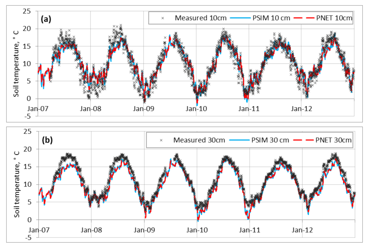
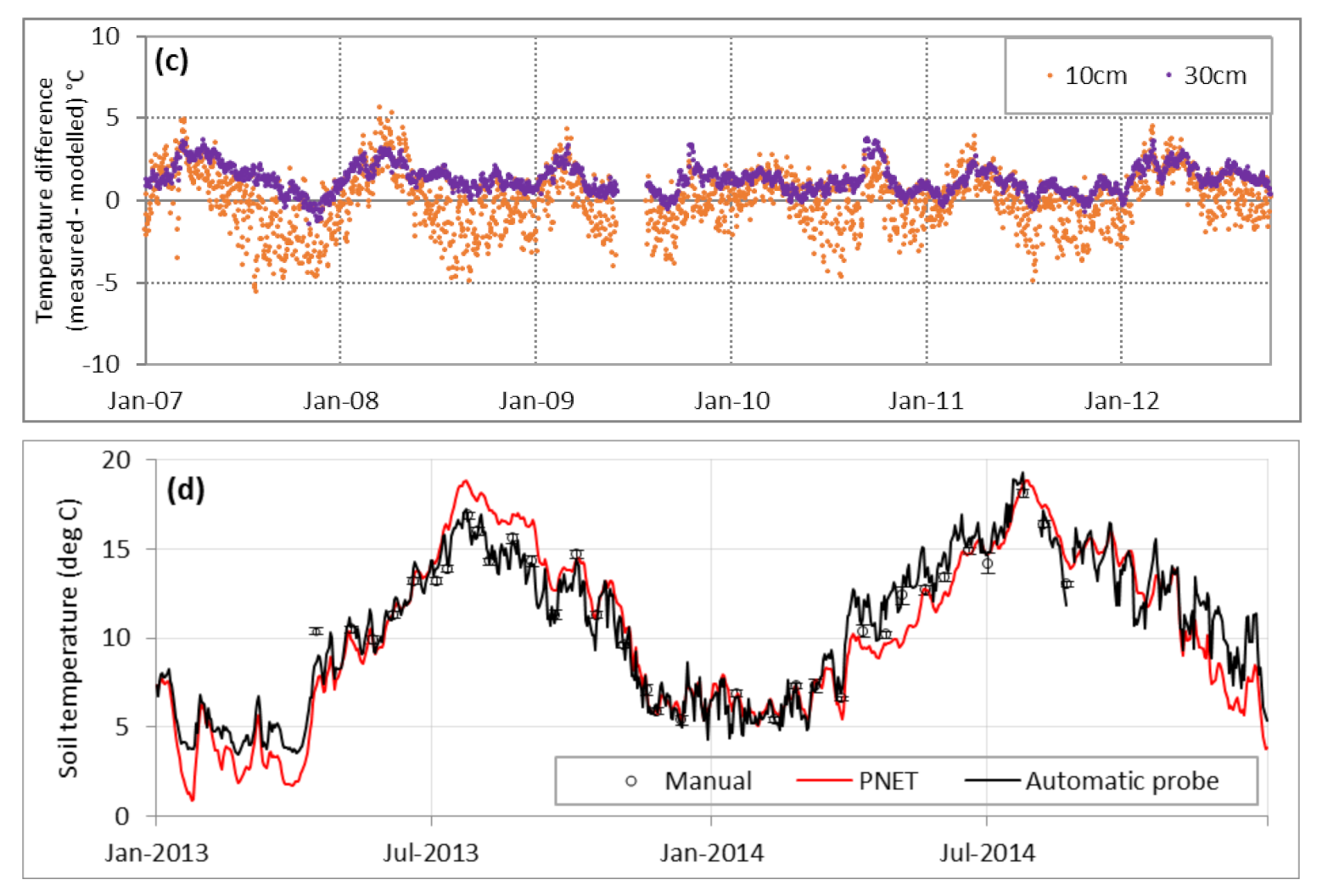
3.1.1. Environmental Conditions

Simulated daily mean soil temperature data at 10 cm depth from January 2007 to December 2012 were similar to measurement data (Figure 1a, y = 0.8x (measured) + 2.1, R2 = 0.90), although they do not quite show the same degree of variation and have a 5–6 °C lower amplitude range, particularly in earlier years. Soil temperatures simulated at 30 cm depth were in closer agreement with measurements (Figure 1b, y = 0.9x − 0.6, R2 = 0.97).
The differences between temperatures simulated with the PnET and PSIM modules were small (<1 °C at 10 cm and <0.5 °C at 30 cm) with near equivalent R2 values. Residual values based on PnET data (Figure 1c) illustrated that the largest differences between measurements and simulations were at 10 cm, mainly in the winter months, when simulated soil temperatures were mostly 1–5 °C higher than measured. Still, there was a good match between both (linear regression: y = 1.1x − 1.1, R2 = 0.90). At 30 cm depth, simulated temperatures were mostly 1–2 °C lower than measured, particularly in the winter. It should be noted that there was also good agreement between soil temperature recorded manually at 10 cm depth near the soil chambers during flux measurements and the mean daily data measured nearby with a fixed probe, strengthening the confidence in measured data (Figure 1d).
Simulated daily mean soil moisture data at 10 cm depth for January 1999 to December 2008 showed a general agreement with available measurements from 1999–2003 (Figure 2), including during the dry summer of 2003 (y = 0.5x + 23.7, R2 = 0.59). However, simulated values were only 2–5% higher in summer and 2–3% lower in winter. Data simulated with PSIM and PnET were similar except during summer 2003 when PSIM simulated lower soil moisture values, closer to measurements. Spikes of high simulated soil moisture (60–65%) from both modules indicate occasions when heavy rainfall has caused surface water to accumulate in the model, although this is not observed at the site, probably because of a slight slope or due to preferential flows that were not visible in the soil profiles used for initialisation.

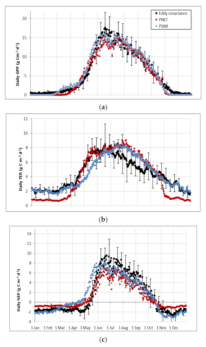
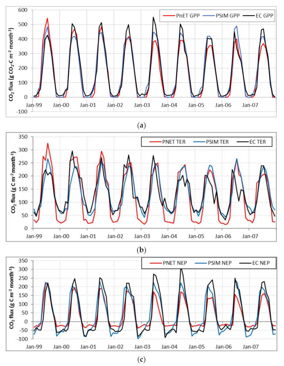
3.1.2. Ecosystem CO2 Fluxes

Annual totals of GPP, TER and NEP for 1999–2007 derived from EC were compared to simulations using either the PnET or PSIM modules after parameter adjustment (Table 4). The differences between mean measured annual values and those simulated by PnET were less than 15% (−8.5%, −6.7% and −14.1%, for GPP, TER and NEP, respectively). Interestingly, underestimation of GPP (and consequently NPP) occurred particularly in the years 2003 and 2006 and did not fully recover in the subsequent years. Closer agreements were obtained with PSIM, with differences between mean measured and simulated values of less than 1% for each CO2 flux component, with no particular high divergence in specific years. While PSIM standard deviations were smaller than those for EC measurements, indicating a low sensitivity to inter-annual variations in environmental influences, PnET deviation was similar for TER and NEP but higher for GPP, reflecting an overestimation of drought susceptibility.
Statistical analysis of annual GPP, TER and NEP totals for 1999–2007 using ModEval [46] showed lower RMSE values when using the PSIM module (7.8, 10.7 and 19.5% for GPP, TER and NEP, respectively) than when using PnET (14.8, 10.9 and 37.4%, respectively) (Table 5a). However, the RMSE values for both modules were all within the 95% confidence intervals of the measured values, and the t-test showed no significant difference between the mean simulated and measured values. Modelling efficiency (ME) values were negative for these annual PnET simulations and coefficients of determination (CD) < 1, which indicates that the PnET-simulated annual totals described the data less well than the mean of the observations, and emphasises that the measured inter-annual variations were not well simulated. PSIM also had negative ME values (though closer to zero) but CD values > 1, which indicates that this model described the measured data better than the mean of the measurements.
Simulated monthly totals for GPP, TER and NEP show a better fit to measured equivalents with high positive ME, CD > 1, no significant bias and high correlation (Figure 3, Table 5b) than annual data (Table 5a). Monthly GPP was particularly well simulated with an ME of 0.94 using PSIM and 0.92 using PnET. RMSE% values were large, particularly for NEP, but were all within the measured 95% confidence intervals, and t-test of mean difference also showed no significant bias in each case. Whereas PnET simulated a reduced GPP and TER in 2003, which was a dry year with Feb–Oct rainfall 50% of the average for that period and high summer temperatures (maximum 33.8 °C), the EC measurements indicated that GPP and TER were higher than average. Although there was a reduction in moisture in the upper soil layers (Figure 2), the site has heavy clay soil (see Table 2) and the previous year was wet with an above average annual rainfall of 1094 mm, suggesting trees had access to subsurface water not represented in the model. PSIM simulations showed little change in GPP for 2003 over the previous year.
The seasonal patterns of the daily GPP averaged over 1999–2007 were quite well simulated by both PnET and PSIM (Figure 4a). Understorey plants produce leaves earlier than canopy trees, and PSIM is able to model the two plant cohorts separately. However, the averaged data from EC suggest that PSIM overestimated this GPP contribution by a factor of approximately 2 during March, although the overestimation is small in comparison with total annual GPP. For TER (Figure 4b), averaged values from the PnET module were closest to measurements in spring and early summer when respiration increases rapidly during canopy growth (April–July), whereas averaged PSIM values were closest in late autumn and winter (November–March). Simulated NEP (the difference between GPP and TER) combines the differences of the other two values (Figure 4c). Averaged daily PSIM NEP showed the largest differences from EC NEP values during May due to a poor match with TER, but a better match with TER during winter months resulted in PSIM producing averaged annual total NEP values close to those measured. These net values are arguably the most important as they determine whether the ecosystem is a net sink or source of CO2 for the year.
Differences between measured and simulated daily GPP, TER and NEP (i.e., residuals) were calculated using the PnET and PSIM modules for 1999–2007 (Figure S1). For each component (GPP, TER and NEP), residuals were mostly between ±5 g C m−2 d−1 for both PnET and PSIM, but the summer residuals were larger in many years, with a maximum GPP residual of −13 g C m−2 d−1 in 2006. Residual TER values showed the clearest distinction between PnET and PSIM, mainly due to the absence of autotrophic soil respiration from roots during winter in PnET simulations. The years 2004 and 2006 show the largest summer residuals (negative) for TER from both modules.
The PnET and PSIM module parameters were adjusted to optimise the fit of the simulations to measurements of annual EC data for GPP, TER and NEP for the period 1999–2007. For the evaluation period, simulations using these parameters were less meaningful because disturbances such as infestations of defoliating moth caterpillars in 2009 and 2010, which are not considered in the simulations, reduced the GPP, TER and, to a lesser extent, NEP, especially in 2010 [28]. It also seems that EC measurements during 1999 to 2010 also showed a significant long-term decrease in annual GPP (−46.1 g C m−2 year−1, p < 0.01) and annual TER (−44.7 g C m−2 year−1, p < 0.001), with no resultant trend for NEP [29]. These decreasing trends in annual GPP and TER are also represented in the simulations (Figure 3), although this might be partly due to the thinning event in 2007. Simulated annual values show larger declines when using PnET (from linear regression: −86.4 g C m−2 year−1 for GPP, R2 = 0.83, and −48.4 g C m−2 year−1 for TER, R2 = 0.87) than when using PSIM (from linear regression: −26.0 g C m−2 year−1, R2 = 0.52, and −21.7 g C m−2 year−1, R2 = 0.55, respectively) (see also Section 3.3).

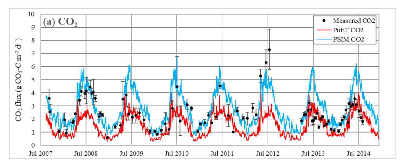
3.1.3. Soil CO2 Effluxes

Measured soil CO2 effluxes occasionally showed large variation between chambers, as indicated by the error bars in Figure 5a, but the seasonal cycle was clear, from a minimum of 1 g C m−2 d−1 in winter to a maximum of 4–6 g C m−2 d−1 in summer. The seasonal cycle in the measured effluxes was well reproduced by the simulated mean daily CO2 efflux, as indicated by the high correlation coefficients for monthly values in Table 5c, although the PSIM module estimated CO2 effluxes up to two times greater than the PnET module (Figure 5a). The PnET module substantially underestimated the mean daily soil CO2 effluxes measured during 2008–2012 (significant bias in mean monthly values, M, in Table 5c) but better matched measurements in 2013–2014 (no significant bias). In contrast, the monthly statistics in Table 5c show that PSIM module results more closely matched 2008–2012 measurements (ME = 0.38, CD = 1.20), but significantly overestimated the smaller soil CO2 effluxes measured in 2013–2014.
PnET-simulated annual total soil CO2 effluxes from 1999–2007 (before thinning) averaged 619 g C m−2 year−1 (range 546–745 g C m−2 year−1), whereas equivalent PSIM-simulated effluxes averaged 1042 g C m−2 year−1 (range 979–1081 g C m−2 year−1). The proportion of simulated annual soil CO2 effluxes contributed by autotrophic respiration when using PSIM was 27.5% compared to 32.3% for PnET. For 2008–2014, averages of 547 g C m−2 year−1 were obtained using PnET and 1018 g C m−2 year−1 using PSIM, compared to a measured value of 807 g C m−2 year−1 (Table 6).

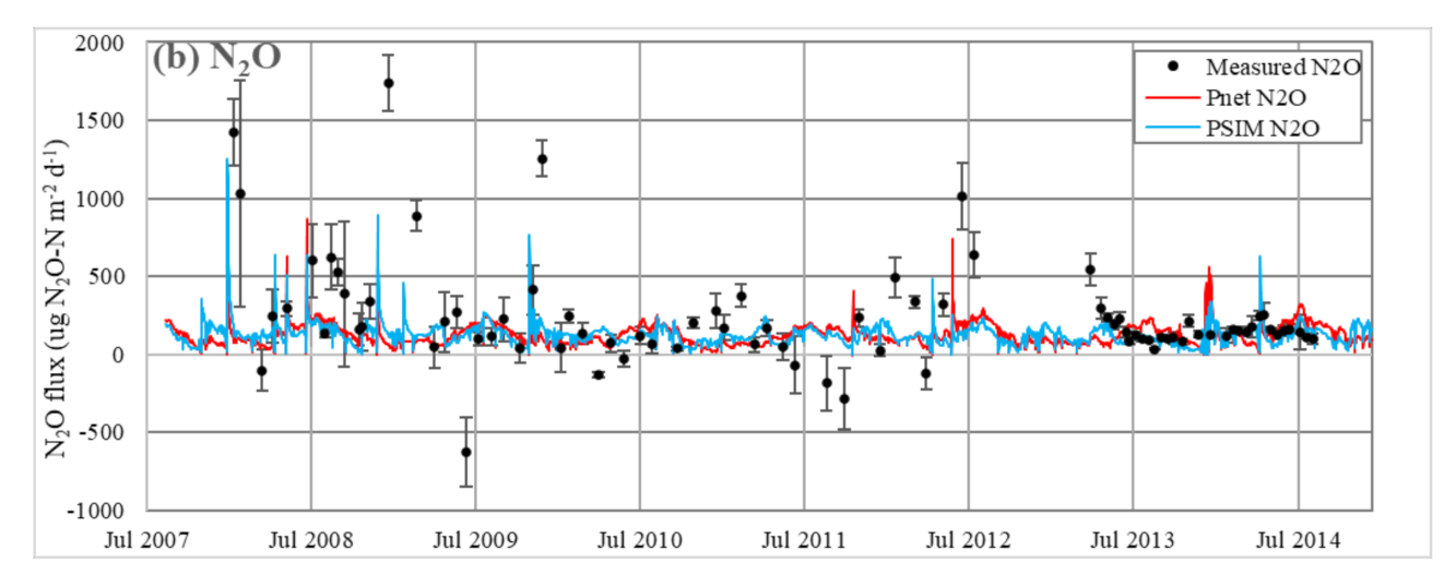
3.1.4. Soil Gaseous N Fluxes

Daily soil N2O fluxes simulated with PnET showed seasonality, ranging from 30–50 µg N m−2 d−1 to summer peaks of 200–300 µg N m−2 d−1 with rain-related spikes on several occasions (Figure 5b). Excluding rain-related spikes, PnET N2O simulations showed a positive correlation with temperature, (r = 0.53, p < 0.01), resulting in high values in the summer; similarly, PSIM N2O simulations were not correlated with temperature (r = 0.04) and the timing of annual maximum values varied from year to year. Measured soil N2O fluxes showed much greater variation and no obvious seasonality, particularly during 2008–2012, and there was no correlation with temperature [50]. On occasions, negative N2O fluxes were measured, but the LandscapeDNDC version used could not simulate soil uptake of N2O. Peak effluxes of 500–1700 µg N m−2 d−1 were measured (Figure 5b). Under wet soil conditions, both PnET and PSIM simulated short-lived spikes in N2O fluxes of 700–900 µg N m−2 d−1 that did not necessarily coincide in time, magnitude or with measured spikes. For example, in early January 2014, PnET simulated N2O fluxes of 600 µg N m−2 d−1, but only fluxes of 300 µg N m−2 d−1 were simulated by PSIM. Annual N2O fluxes, adjusted to calendar year and estimated from approximately monthly measurements, ranged from 15.4 to 156 mg N m−2 year−1 during 2009–2011 [50] and 57.4 mg N m−2 year−1 in 2013 measured during this study. Fluxes simulated with PnET and PSIM for the same periods were less varied but within the range of 38.9–55.2 mg N m−2 year−1 and 36.9–52.3 mg N m−2 year−1, respectively (Table 6), and closer to the measured annual flux for 2013.
Monthly measured N2O flux totals were compared with those simulated using PnET and PSIM modules with data from 2008–2012 analysed separately from 2013–2014 data (Table 5c). For both PnET and PSIM, the RMSE% values were large, and for 2008–2012, within the 95% confidence intervals of the measured means despite being >100%, due to larger variations in the fewer measured values than in 2013–2014 when the RMSE was significantly different from measurements. ME was negative and CD < 1 for 2013–2014 simulated N2O flux results from both models, suggesting that in this case, the measured data are better described by the mean. However, both simulations showed CD values > 1 for 2008–2012, which highlights the impact of the high degree of variability in soil N2O fluxes and the relative frequency of measurements. It also indicates there is considerable uncertainty in annual totals calculated from these measurements.

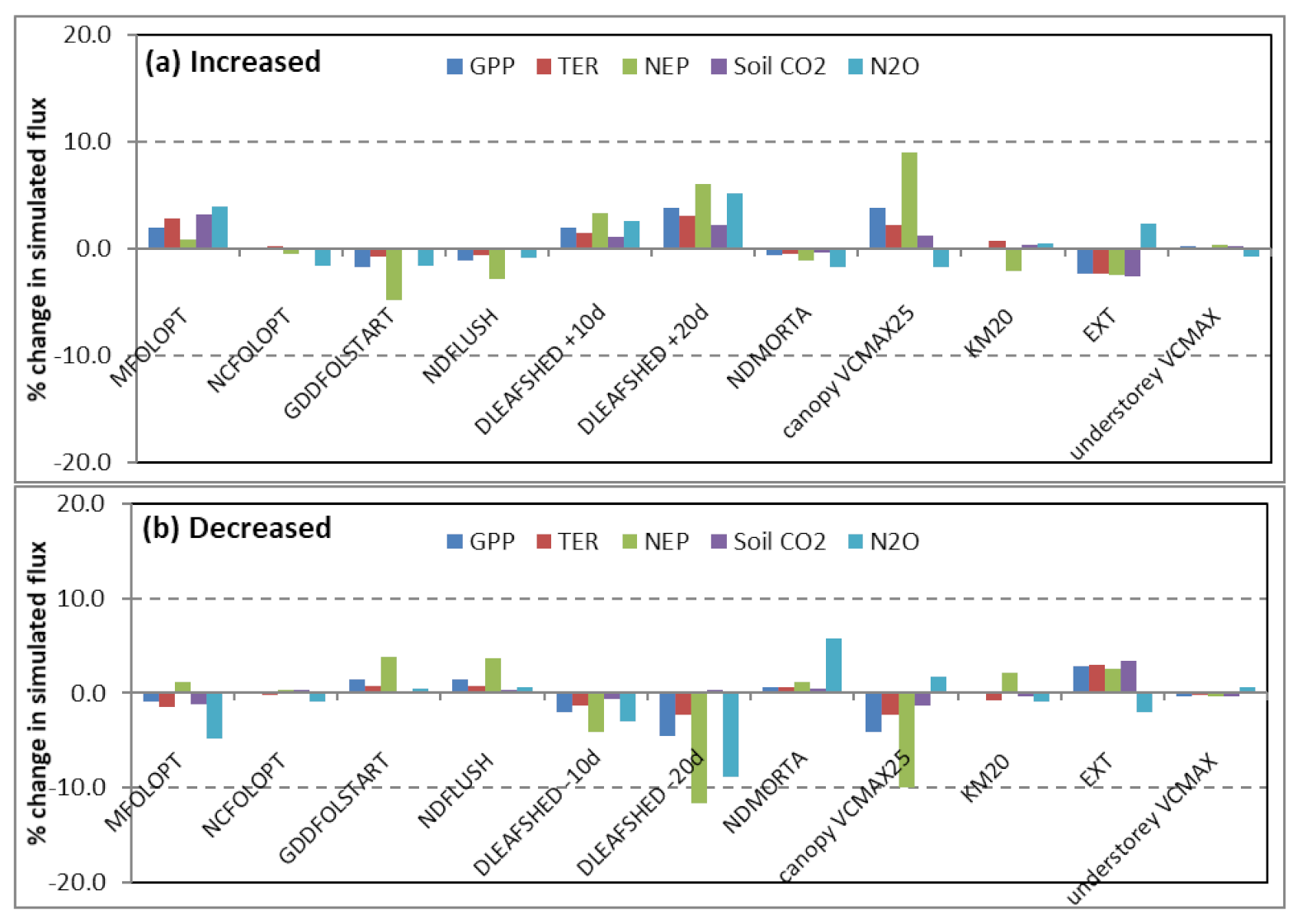
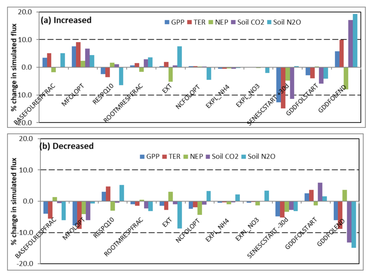
3.2. Model Sensitivity Analysis
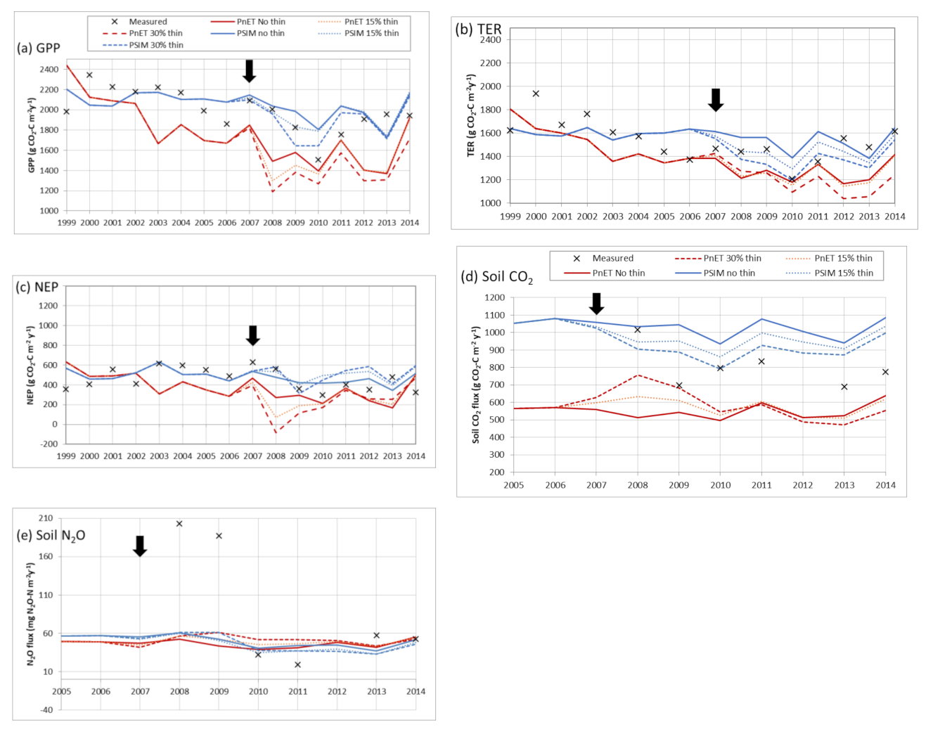
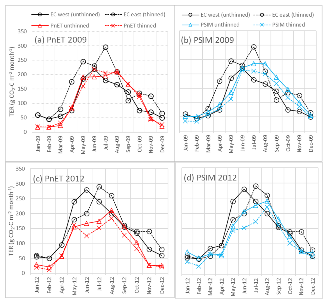
Figure 6 illustrates the effect of changes to key input variables and parameters on annual GPP, TER, NEP and soil CO2 and N2O fluxes simulated using PnET and averaged over 1999–2007 (Table S1a). The simulated annual CO2 flux components showed rather little sensitivity to changes in soil parameters, but more to changes in temperature and precipitation.
Changing the bulk density (BD) input values by 10% produced a disproportionate change in N2O fluxes. This value controls the initial organic C (and N) stock in the soil as well as soil porosity. A higher BD (given in g cm−3) results in higher organic C content (input to model as a fraction of BD) and lower porosity (input as % of BD), which provides more substrate for microbes and results in more anaerobic conditions during wetting. The hydraulic conductivity of the soil was uncertain, as it was not determined. Although the soil is clay-rich, tree roots promote conduits for water percolation. Values of 10 and 100 times higher than the selected value of 0.0006 mm min−1 were shown to reduce the simulated gas fluxes by less than 5%. Changing the daily climate variables of minimum, maximum and mean temperature (in a single simulation) or precipitation by ± 10% produced changes to gas fluxes of <10%, with a shift from litter layer to mineral soil nitrification due to reduced microbial activity in the litter layer. Changes in N deposition of ± 10% changed soil N2O fluxes by less than 4%. Increasing N deposition by 100% to 2.46 g N m−2 year−1, which is similar to values of 2.0–3.5 g N m−2 year−1 recorded for a broadleaved forest at Hoeglwald in central Europe [54], resulted in large, simulated increases in N2O fluxes of 17.7%. This analysis therefore showed that simulated soil fluxes were particularly sensitive to initial organic C content (via bulk density) and to factors that control soil moisture and thereby anaerobic conditions, i.e., bulk density and field capacity. It also showed that stand-scale CO2 fluxes were relatively insensitive to changes in input values, which may explain the low interannual variations simulated.
Model sensitivity to selected PnET parameters is shown in Figure 7 (Table S1b). Changes of ±10% to GDDFOLEND (daily temperature sum for end of foliage growth; see Table 3) produced >10% change in all simulated soil fluxes; increasing SENESCSTART (leaf death timing) by 30 days decreased simulated GPP, TER and soil CO2 fluxes by >10%, which indicates the importance of defining the start and end of the growing season to simulated respiration and soil processes. Changing these parameters affects the allocation of carbon at the end of the year and hence the amount available for leaf development the following year, which has a cumulative effect after several years. However, SENESCSTART defines a day of year and therefore is not comparable to % change in outputs, whereas changing GDDFOLEND affects leaf N uptake and therefore the intensity rather than timing of soil emissions.
Figure 8 shows model sensitivity to PSIM parameters (Table S1c). No single parameter had a disproportionate effect on the simulated results. Comparison of the PSIM module with and without a vegetation understorey, modelled as different sets of carbon pools (as defined in Table 1), showed that the understorey contributed 20%, 17% and 20% of simulated TER, GPP, and soil CO2 emissions, respectively, and 14% of simulated soil N2O emissions. However, the understorey vegetation characteristics vary substantially across the Inclosure; there are few measurements of understorey parameters to inform the choice of values, and no measurements to evaluate its proportional contribution to fluxes. Therefore, there are considerable uncertainties in the contribution of the understorey to the TER, GPP and soil fluxes of CO2 and N2O in this forest.

3.3. Thinning

Following 30% thinning, annual GPP simulations showed an initial decline in both modules, and then a recovery over several years (Figure 9a). Using the PSIM module, the largest difference from unthinned simulations was in 2009 with a 17% reduction in GPP, which recovered fully to that of the unthinned by 2013. For PnET, the largest difference from unthinned simulations was in 2008 with a 20% reduction and, although this difference reduced by 2010, it maintained a similar difference (4–11% lower) for the duration of the simulations. The initial small change in GPP after thinning in the PSIM module more closely fit the measured changes than did the PnET module equivalent, which had a larger initial decline. Annual TER simulation (Figure 9b) also showed a decline in PSIM following the thin (maximum difference 15% in 2009), which recovered gradually but not completely by the end of the study (6% difference in 2014). For PnET, simulated TER increased slightly (by 5%) in 2007 and 2008 after thinning, before declining, and the difference in simulated values continued to increase thereafter to 12% by 2014. For PSIM, the maximum change in NEP was small (28%) compared to PnET, which showed a maximum reduction in NEP of 131%, resulting in negative NEP (i.e., a net loss of CO2) in 2008 (Figure 9c). PnET simulations produced a 47% increase in soil CO2 efflux in 2008, whereas PSIM simulated a 12% decrease, increasing to 15% in 2009 and 2010 (Figure 9d). Both modules also showed an increase in simulated N2O emissions after the thin, and although relatively small in absolute values, the proportional increase was larger in PnET (39%) than for PSIM (17%) (Figure 9e). It should be noted that although soil CO2 and N2O flux measurements are shown in Figure 9d,e, these were from the Tower Site and will not have been directly affected by the thinning.
For the 15% simulated thinning, the differences in simulated fluxes followed the same trends as those produced by the 30% thin. For PSIM simulations, the 15% thin closely matches whole-stand EC measurements immediately after the thin in 2007–2009 (Figure 10a–c). The significant decrease in both measured GPP and TER in 2010 has been attributed to a defoliating caterpillar infestation [29], which may explain a poor model fit for 2010 and possibly subsequent years. However, both PSIM and PnET simulations showed a decrease in GPP and TER in the same year, suggesting an environmental effect may also have contributed to the low measured values in 2010.
Wilkinson et al. [45] reported changes in measured stand CO2 fluxes after the thinning event in 2007; while fluxes in 2008 were little changed, there were markedly increased respiration rates in 2009 from the eastern thinned area, likely to be caused by the decomposition of brash and stumps. Monthly measured TER data partitioned into eastern (thinned) and western (unthinned) sectors from [45] in 2009 and 2012 were compared with 0% and 30% thinning simulated using PnET and PSIM (Figure 10). To account for the small differences in weather conditions when the wind is from east or west, simulated daily data were separated into east and west sectors. In 2009, two years after thinning, measured TER was predominantly higher throughout the year during easterly winds. However, PnET-simulated monthly TER hardly differed for 0% and 30% thinning and was most similar to measured fluxes from the west sector (Figure 10a). In contrast, PSIM-simulated TER showed a clear reduction for 30% thinning, compared with 0% thinning between January and November 2009, and higher simulated TER values after June than those measured from the west (Figure 10b). In 2012, 5 years after the thinning, measured TER values were similar in the western and eastern sectors, except that the summer peak in the eastern sector lagged behind that of the western sector by a month. PnET-simulated TER values were substantially lower than measured values throughout the year and, unlike in 2009, simulated thinning decreased TER slightly between May and October 2012 (Figure 10c). As in 2009, PSIM-simulated TER was reduced by the 30% thinning, particularly in summer months (Figure 10d).
For the above comparison of simulated and measured data, model efficiency (ME) values were consistently >0; coefficient of determination (CD) values were >1 in all PSIM simulations except 0% thinning in 2009 and were <1 in all PnET simulations (Table 7). PSIM produced better simulated monthly results, giving slightly higher CD values and similar or lower RMSE than PnET, except for the 2009 simulations with 0% thinning. However, for both years, the unthinned model output gave a better match to the western sector measured data than the thinned model output did to the eastern sector measured data.

4. Discussion

4.1. Simulation of Environmental Conditions

As soil temperature and soil moisture are major controls on GHG fluxes from soils, accurate simulation of these values is important, especially in the uppermost soil layers (0–30 cm) where most biological activity takes place [55,56]. Simulated soil temperature, using both PnET and PSIM, had a lower annual amplitude than measured data for most years. The only year studied when simulated temperature amplitude exceeded measured amplitude, 2013, had an anomalously dry summer (68 mm, compared with average summer rainfall of 167 mm) and a cold Jan–Mar (average temperature of 3.3 °C, compared with the equivalent for 1995–2013 of 5.8 °C), which suggests a link with climatic conditions. DNDC calculates soil temperature from soil properties including thermal conductivity derived from a combination of solid and water phases, depending on moisture content [34]. It seems that when the moisture content is high, the simulation of soil temperature is less accurate. The small difference of <1 °C in extreme values of PSIM and PnET soil temperatures is probably generated in the ECM air chemistry module due to differences in canopy structure, which causes shading, and evapotranspiration, before soil surface temperatures are calculated in the DNDC soil microclimate module.
Soil moisture measurements at the Straits Inclosure Tower Site have been unreliable at times, especially following dry conditions in the clay-rich soils when cracks reduce the probe accuracy, and spatial variation from proximity to vegetation is expected (relative standard error was 1–6%). As with soil temperature, simulated soil moisture generally showed a reduced seasonal range, with the exception of peaks (often one day long) following heavy rainfall events. The original aim of DNDC was to predict seasonal or annual N2O emissions [16] and therefore the timing of simulated rain events was not important: they start at midnight and continue at the same pre-defined intensity until daily rainfall has finished [37].
The vegetation module takes account of canopy interception and evapotranspiration, and then rainwater saturates the soil, layer by layer, at a rate determined by each layer’s soil hydraulic conductivity (K). Altering K at model setup changes soil moisture during and after rainfall events, but a 100-fold change in K (from 0.0006 to 0.06 mm min−1) only changed simulated soil moisture by 1–2% on most days. Results with the higher input K were still 2–3% different from the measured values and did not affect the simulated soil temperature. However, the effect of simulating rainfall in this way in a clay-rich soil was to create more occasions when surface water accumulates and hence more times when anaerobic conditions were simulated for denitrification. This simplification therefore probably contributed to the overestimation of N2O peak emissions at this site. Many of the studies using combined PnET and DNDC models have involved forests on loams and sandy loams, e.g., [57], for which simplified rainfall and drainage models produced N2O emission values within 4% of measurements in one site studied. Saggar et al. [58] and Li et al. [59] modelled clay-rich agricultural soils with DNDC, and modified soil moisture processes in order to obtain better matches with measured soil moisture and soil drainage. Following field experiments in a temperate oak forest, Liu et al. [60] suggest drought intensity enhances the response of soil respiration to a precipitation pulse, as the length of drought had a greater effect on soil CO2 efflux than the amount of precipitation. This is not represented in the model used here but would be important for modelling climate change scenarios.

4.2. Vegetation Species Parameters and Simulation of CO2 Fluxes

Simulations using the standard species parameters for pedunculate oak (Q. robur) resulted in annual GPP values approximately half those estimated by EC, indicating that customisation was required. However, if the model is to be applicable at more than one site, the number of parameters altered should be minimal. For PnET, the principal control on a species’ C uptake is the parameter AMAXB (optimal photosynthetic rate), together with MFOLOPT (optimal foliage biomass), which determines LAI. These two parameters directly control the simulated GPP values and were changed incrementally until annual EC GPP was matched. Simulated autotrophic respiration is summed from the growth and maintenance of three C pools (leaves, wood and roots), and four parameters define the fractions of photosynthesis and biomass used to calculate respiration, together with a Q10 and three C allocation parameters. There is no parameter that controls heterotrophic soil respiration. Therefore, matching TER from EC data was less straightforward and required balancing with resultant NEP values derived from GPP and TER. Although sub-optimal GPP values may be necessary to ensure both TER and NEP are optimised, it is most likely that there will be a better fit for GPP than both TER and NEP when modelling with PnET. For PSIM, there are also two key parameters that control photosynthesis (VCMAX25 and MCFOLOPT), but only one key parameter that controls respiration (KM20), which simplifies the optimisation process.
These gas exchange parameter values were selected to match averaged annual values for GPP, TER and NEP. Changing phenology-related parameters helped match seasonal variations but not inter-annual variations, particularly in PSIM data. PnET uses daily temperature, through cumulative growing degree days (GDD), to control the start and end of leaf unfolding, whereas PSIM only uses GDD at the start and a parameter-defined number of days to complete the process. Similarly, the timing and length of leaf fall remain constant for each year in PSIM, but in PnET these can vary according to conditions. Thus, PnET simulated a larger inter-annual range (205–252 days of non-zero C uptake) in growing season length (GSL) compared to PSIM canopy trees (210–248 days), which contributes to differences in their simulated inter-annual variations. PnET and PSIM both show a positive correlation between GSL and simulated annual GPP (PSIM, r = 0.78, p < 0.01; PnET, r = 0.52, p < 0.05). GSL has been reported by Goulden et al. [61] to be a controlling factor on annual GPP in a deciduous forest in New England. However, Wilkinson et al. [29] did not find any such correlation between observed GSL and EC GPP. The strongest correlation they found to explain inter-annual variation was between peak LAI and GPP in Straits data from 1999 to 2010. Conversely, simulated LAI shows very little annual variation in peak values (PnET range: 4.85–5.79; PSIM canopy range: 5.47–5.86, understorey: 3.16–3.92, total: 8.64–9.69) and no correlation with simulated GPP or TER.
Thus, it seems the inability to vary peak LAI appropriately in both models may cause the poor match in inter-annual variability. However, the exfoliating caterpillar infestations of 2009–2010 were known external factors that affected the forest LAI and therefore GPP, and there may have been other factors (e.g., disease, storm damage) that are not simulated but account for some of the mismatch. No correlation was found between annual rainfall and GPP in either PnET or PSIM, but drought stress affected PnET outputs more than those of PSIM in 2003, although EC measurements showed the Straits Inclosure was not adversely affected.
The annual biomass increment for the Straits Inclosure between 1997 and 2011 was estimated as 347 g C m−2 year−1 from measurements of the canopy trees [29], although this was an underestimate of total stand NEP as it did not include the understorey. Simulated biomass from end of year C pools of wood and coarse roots, following loss of leaves and fine roots with no thinning, gave broadly comparable values for an average annual increment between 1999 and 2011 of 374 g C m−2 year−1 using PnET and 439 g C m−2 year−1 using PSIM. At the end of 2010, biomass was estimated from measurements as 16.5 kg C m−2 (Forest Research, personal comm.), which compares well with simulated values of 16.7 kg C m−2 using PNET and 18.4 kg C m−2 using PSIM (of which 1.5 kg C m−2 was understorey).

4.3. Simulating Soil Gas Fluxes and Measurement Uncertainty

Soil chamber measurements are known to be subject to errors and both spatial and temporal variability are expected [62,63]. Measurements during this study were made once every 2–4 weeks; therefore, estimated annual fluxes may have compounded errors resulting from diurnal and short-term temporal variations. Overall, the results show that PSIM-simulated soil CO2 effluxes matched the measured effluxes more closely than those simulated by PnET. PSIM gave a mean ratio of soil CO2:TER of 0.67 for 2008–2011 with and without thinning, which is similar to the mean ratio of 0.61 and 0.60 in measurements by Yamulki and Morison [50] and Heinemeyer et al. [64], respectively. The equivalent ratio for the PnET simulations was 0.47 for 2013–2014. PSIM simulated a greater annual maximum total root mass of 0.9 kg DW m−2 than did PnET (0.25 kg DW m−2) due to the addition of understorey vegetation. We suggest that the differences in total CO2 efflux are largely due to the simulation of root exudates that occurs in PSIM, generating extra substrates for heterotrophic respiration, but is not modelled in PnET.
Chamber measurements of soil N2O fluxes are subject to similar measurement errors as soil CO2 effluxes [65,66]. The overestimation of N2O peak fluxes by the model has been discussed above as an effect of the simplification of rainfall simulation and resulting moisture content. The presence of the understorey affects the intensity of simulated fluxes, rather than seasonal pattern, and is linked to simulated N uptake. A constant N deposition was assumed in the simulation, but Vanguelova et al. [67] report decreases in NH4-N throughfall at Alice Holt from 1995 to 2006 of approximately 0.7 NH4-N eq ha−1 year−1, which would result in a decrease in N2O fluxes if continued during the period simulated here and may also have contributed to the mismatch between measured and modelled data.
The inability to model the uptake of N2O is a further simplification that contributes to poor agreement with measurements.

4.4. Simulating Thinning/Response to Management Change

Evaluating the simulated thinning event alone was complicated by the fact that thinning took place over only half of the plantation and there was only one EC tower to measure the change. Furthermore, there is heterogeneity across the site, particularly in the understorey species and density, which has not been quantified. Differences in weather conditions coming from the western and the eastern sectors contribute to different GPP and TER rates in addition to the thinning status. However, the PnET-simulated negative NEP in 2008 (Figure 9c) was caused by simulated GPP being too low. Measured TER was higher in the thinned sector from 2009 (i.e., after a lag, Figure 10a); although PnET also simulated an increase in TER after thinning (Figure 9b), principally as a result of increased soil respiration (Figure 9d), this started in 2007 and by 2009 TER had returned to unthinned sector values. In contrast, PSIM simulated a decrease in TER from the 2007 thin. The main difference between the modules was the simulated soil respiration, which increased with PnET due to increased litter input, causing higher heterotrophic respiration from increased mineralisation, but decreased in PSIM because mineralisation remained unchanged and root respiration decreased. Both modules simulated an increase in soil N2O fluxes following the thin, which is in agreement with Yamulki and Morison [50], in which the least thinned areas of the Straits Inclosure recorded the lowest soil N2O fluxes during 2010–2012.

5. Conclusions

LandscapeDNDC with the two different tree growth modules, PnET and PSIM, was evaluated for application in an oak forest in southern England by modifying a limited set of species parameters that define tree physiology. The PnET module simulated annual GPP, TER and NEP rates averaged over 1999–2007 to within 8.5%, 6.7% and 14.1%, respectively, of values derived from EC measurements, which is within the estimated uncertainty of the EC method of 10–15% suggested by Oren et al. [48]. The PSIM module, which included an understorey component, simulated these mean annual data to within < 1%. For both modules, the measured inter-annual variability of GPP, TER and NEP was not well simulated, and comparison with measurements indicated negative modelling efficiency (ME) values. However, when monthly CO2 fluxes were compared, the model efficiency for PnET and PSIM improved to positive values. These annual and monthly comparisons suggest that while the main processes in the forest CO2 balance are included, neither module has appropriate sensitivity to key drivers to respond to interannual variations.
Annual soil CO2 fluxes were consistently underestimated by PnET by 32% compared with average soil chamber measurements, but were overestimated by 26% by PSIM. Measured soil N2O fluxes exhibited considerable inter-annual variation of 15.4–156 mg N m−2 year−1, which was not reproduced by PnET or PSIM, but in both cases simulated annual totals were of the same order of magnitude as measurements (PnET: 38.9–55.2 mg N m−2 year−1 and PSIM: 36.9–60.3 mg N m−2 year−1). Comparison between monthly simulated and measured N2O soil flux data showed poor agreement for both modules. For soil CO2 fluxes, PSIM produced better results when compared with measurements from 2008–2012.
For soil N2O fluxes, LandscapeDNDC was most sensitive to initialisation values of bulk density, which also affects soil organic carbon content and field capacity. Of the climate variables, decreasing the temperature by 10% had a greater effect on N2O emissions than increasing temperature or changing precipitation by 10%. The PnET parameter to which simulated soil N2O and CO2 fluxes were most sensitive, increasing over the duration of the simulation, was GDDFOLEND, which defines the cumulative temperature required to reach maximum leaf area. There was no single PSIM parameter to which simulated fluxes were particularly sensitive, but inclusion of the understorey contributed 14–22% to simulated flux outputs of GPP, TER, soil CO2 and N2O.
The simulation of forest thinning showed that PSIM produced a better match to measured GPP and NEP data than PnET, although the latter simulated a more realistic response for the TER rate through increased soil respiration. Both modules reproduced monthly variations in TER well for two separate years following thinning (PnET ME = 0.46 and 0.18; PSIM ME = 0.45 and 0.60), but neither module reproduced the details of the measured time course. The simulated increases in N2O gas emissions could not be assessed accurately but agreed broadly with observations made at the site by Yamulki and Morison [50].
This study shows that the LandscapeDNDC model can simulate monthly and averaged annual ecosystem CO2 fluxes measured at the Straits Inclosure well when key parameters have been optimised for local conditions. The PSIM module performed better than PnET and its ability to simulate the significant understorey component present at the site may have contributed to the improvement, although there is insufficient information to provide robust understorey parameter values or to evaluate the understorey simulation. While monthly soil CO2 fluxes have been shown to be well simulated by PSIM, particularly compared to 2008–2012 measurements, N2O fluxes and variability were not. Improvements to the model in order to better simulate the observed inter-annual variability would be necessary before either module is used to predict impacts of changes due to climate and/or management at this site.

Supplementary Materials

The following are available online at https://www.mdpi.com/article/10.3390/f12111517/s1, Figure S1. Daily residual values (measured–simulated) for: (a) GPP, (b) TER and (c) NEP at the Straits Inclosure, modelled with PnET (red circles) and PSIM (blue circles) modules 1999–2007. Table S1. Sensitivity test results showing % change in simulated annual total GHG fluxes averaged over 1999–2007 for (a) input variable changes simulated with PnET (see Table 1 and Table 2 for initial input values), (b) parameter value changes simulated with PnET and (c) parameter value changes simulated with PSIM. Parameter value units are given in Table 3. Changes >10% shaded.

Author Contributions

Conceptualisation, S.Y. and E.H.; methodology, S.Y. and S.M.-H.; software, E.H.; validation, S.M.C., J.I.L.M., R.G. and S.M.-H.; formal analysis, S.M.C.; investigation, S.M.C.; resources, K.C.C. and S.Y.; data curation, R.G., M.W. and S.M.C.; writing—original draft preparation, S.M.C.; writing—review and editing, J.I.L.M., S.Y., K.C.C. and R.G.; supervision, K.C.C. and S.Y.; funding acquisition, K.C.C. and S.Y. All authors have read and agreed to the published version of the manuscript.

Funding

This research was funded by a College Research and Crossland Scholarship from Royal Holloway, a University of London travel grant, and the Forestry Commission (Forest Research).

Data Availability Statement

Measured data used in this study are available on request from the corresponding author.

Acknowledgments

We wish to acknowledge staff at Royal Holloway, Forest Research and the Institute of Meteorology and Climate Research, KIT, and in particular David Ames for bespoke NOx data logging software, Iñaki Valcarcel for help with soil analyses, Jacqui Brunt for GC analysis, Eric Casella for Straits Inclosure mensuration data and modelling advice, Steffen Klatt and David Kraus for help with LandscapeDNDC, and Ralf Kiese for enabling use of the model.

Conflicts of Interest

The authors declare no conflict of interest.

References

  1. Ciais, P.; Sabine, C.; Bala, G.; Bopp, L.; Brovkin, V.; Canadell, J.; Chhabra, A.; DeFries, R.; Galloway, J.; Heimann, M.; et al. 2013: Carbon and Other Biogeochemical Cycles. In Climate Change 2013: The Physical Science Basis. Contribution of Working Group I to the Fifth Assessment Report of the Intergovernmental Panel on Climate Change; Stocker, T.F., Qin, D., Plattner, G.K., Tignor, M.M.B., Allen, S.K., Boschung, J., Nauels, A., Xia, Y., Bex, V., Midgley, P.M., Eds.; Cambridge University Press: Cambridge, UK; New York, NY, USA, 2013. [Google Scholar]
  2. Pan, Y.; Birdsey, R.A.; Fang, J.; Houghton, R.; Kauppi, P.E.; Kurz, W.A.; Phillips, O.L.; Shvidenko, A.; Lewis, S.L.; Canadell, J.G.; et al. A large and persistent carbon sink in the world’s forests. Science 2011, 333, 988–993. [Google Scholar] [CrossRef] [Green Version]
  3. Finzi, A.C.; Giasson, M.A.; Barker Plotkin, A.A.; Aber, J.D.; Boose, E.R.; Davidson, A.E.; Dietze, M.C.; Ellison, A.M.; Frey, S.D.; Goldman, E.; et al. Carbon budget of the Harvard Forest Long-Term Ecological Research site: Pattern, process, and response to global change. Ecol. Monogr. 2020, 90, e01423. [Google Scholar] [CrossRef]
  4. Thurner, M.; Beer, C.; Santoro, M.; Carvalhais, N.; Wutzler, T.; Schepaschenko, D.; Shvidenko, A.; Kompter, E.; Ahrens, B.; Levick, S.R. Carbon stock and density of northern boreal and temperate forests. Global Ecol. Biogeogr. 2014, 23, 297–310. [Google Scholar] [CrossRef]
  5. Blagodatsky, S.; Yevdokimov, I.; Larionova, A.; Richter, J. Microbial growth in soil and nitrogen turnover: Model calibration with laboratory data. Soil Biol. Biochem. 1998, 30, 1757–1764. [Google Scholar] [CrossRef]
  6. Ingwersen, J.; Butterbach-Bahl, K.; Gasche, R.; Papen, H.; Richter, O. Barometric process separation: New method for quantifying nitrification, denitrification, and nitrous oxide sources in soils. Soil Sci. Soc. Am. J. 1999, 63, 117–128. [Google Scholar] [CrossRef]
  7. Schindlbacher, A.; Zechmeister-Boltenstern, S.; Butterbach-Bahl, K. Effects of soil moisture and temperature on NO, NO2, and N2O emissions from European forest soils. J. Geophys. Res. Atmos. 2004, 109, D17302. [Google Scholar] [CrossRef]
  8. Pilegaard, K.; Skiba, U.; Ambus, P.; Beier, C.; Brüggemann, N.; Butterbach-Bahl, K.; Dick, J.; Dorsey, J.; Duyzer, J.; Gallagher, M. Factors controlling regional differences in forest soil emission of nitrogen oxides (NO and N2O). Biogeosciences 2006, 3, 651–661. [Google Scholar] [CrossRef] [Green Version]
  9. Luo, G.; Brüggemann, N.; Wolf, B.; Gasche, R.; Grote, R.; Butterbach-Bahl, K. Decadal variability of soil CO2, NO, N2O, and CH4 fluxes at the Höglwald Forest, Germany. Biogeosciences 2012, 9, 1741–1763. [Google Scholar] [CrossRef] [Green Version]
  10. Haas, E.; Klatt, S.; Fröhlich, A.; Kraft, P.; Werner, C.; Kiese, R.; Grote, R.; Breuer, L.; Butterbach-Bahl, K. LandscapeDNDC: A process model for simulation of biosphere-atmosphere-hydrosphere exchange processes at site and regional scale. Landsc. Ecol. 2013, 28, 615–636. [Google Scholar] [CrossRef]
  11. Cameron, D.R.; Van Oijen, M.; Werner, C.; Butterbach-Bahl, K.; Grote, R.; Haas, E.; Heuvelink, G.B.M.; Kiese, R.; Kros, J.; Kuhnert, M.; et al. Environmental change impacts on the C- and N-cycle of European forests: A model comparison study. Biogeosciences 2013, 10, 1751–1773. [Google Scholar] [CrossRef] [Green Version]
  12. Aber, J.D.; Federer, C.A. A generalized, lumped-parameter model of photosynthesis, evapotranspiration and net primary production in temperate and boreal forest ecosystems. Oecologia 1992, 92, 463–474. [Google Scholar] [CrossRef]
  13. Aber, J.D.; Ollinger, S.V.; Federer, C.A.; Reich, P.B.; Goulden, M.L.; Kicklighter, D.W.; Melillo, J.; Lathrop Jr, R.G. Predicting the effects of climate change on water yield and forest production in the northeastern United States. Clim. Res. 1995, 5, 207–222. [Google Scholar] [CrossRef]
  14. Grote, R. Sensitivity of volatile monoterpene emission to changes in canopy structure: A model-based exercise with a process-based emission model. New Phytol. 2007, 173, 550–561. [Google Scholar] [CrossRef] [PubMed]
  15. Grote, R.; Kiese, R.; Grünwald, T.; Ourcival, J.; Granier, A. Modelling forest carbon balances considering tree mortality and removal. Agric. For. Meteorol. 2011, 151, 179–190. [Google Scholar] [CrossRef]
  16. Li, C.; Frolking, S.; Frolking, T.A. A model of nitrous oxide evolution from soil driven by rainfall events: 1. Model structure and sensitivity. J. Geophys. Res. 1992, 97, 9759–9776. [Google Scholar] [CrossRef]
  17. Li, C.; Trettin, C.; Sun, G.; McNulty, S.; Butterbach-Bahl, K. Modeling carbon and nitrogen biogeochemistry in forest ecosystems. In Proceedings of the 3rd International Nitrogen Conference, Nanjing, China, 12–16 October 2004; pp. 893–898. [Google Scholar]
  18. Werner, C.; Butterbach-Bahl, K.; Haas, E.; Hickler, T.; Kiese, R. A global inventory of N2O emissions from tropical rainforest soils using a detailed biogeochemical model. Glob. Biogeochem. Cycles 2007, 21. [Google Scholar] [CrossRef]
  19. Status and trends in sustainable forest management in Europe. In Proceedings of the Forest Europe and FAO: State of Europe’s Forests 2015, Ministerial Conference on the Protection of Forests in Europe, FOREST EUROPE Liaison Unit, Madrid, Spain, 20–21 October 2015; p. 314.
  20. Pilli, R.; Grassi, G.; Kurz, W.A.; Fiorese, G.; Cescatti, A. The European forest sector: Past and future carbon budget and fluxes under different management scenarios. Biogeosciences 2017, 14, 2387–2405. [Google Scholar] [CrossRef] [Green Version]
  21. Porté, A.; Bartelink, H. Modelling mixed forest growth: A review of models for forest management. Ecol. Model. 2002, 150, 141–188. [Google Scholar] [CrossRef]
  22. Groenendijk, M.; Dolman, A.; Van der Molen, M.; Leuning, R.; Arneth, A.; Delpierre, N.; Gash, J.; Lindroth, A.; Richardson, A.; Verbeeck, H. Assessing parameter variability in a photosynthesis model within and between plant functional types using global Fluxnet eddy covariance data. Agric. For. Meteorol. 2011, 151, 22–38. [Google Scholar] [CrossRef]
  23. Molina-Herrera, S.; Grote, R.; Santabárbara-Ruiz, I.; Kraus, D.; Klatt, S.; Haas, E.; Kiese, R.; Butterbach-Bahl, K. Simulation of CO2 Fluxes in European Forest Ecosystems with the Coupled Soil-Vegetation Process Model “LandscapeDNDC”. Forests 2015, 6, 1779–1809. [Google Scholar] [CrossRef] [Green Version]
  24. Perkins, D.; Uhl, E.; Biber, P.; du Toit, B.; Carraro, V.; Rötzer, T.; Pretzsch, H. Impact of climate trends and drought events on the growth of oaks (Quercus robur L. and Quercus petraea (Matt.) Liebl.) within and beyond their natural range. Forests 2018, 9, 108. [Google Scholar] [CrossRef] [Green Version]
  25. Landuyt, D.; Perring, M.P.; Seidl, R.; Taubert, F.; Verbeeck, H.; Verheyen, K. Modelling understorey dynamics in temperate forests under global change—Challenges and perspectives, Perspect. Plant Ecol. Evol. Syst. 2018, 31, 44–54. [Google Scholar] [CrossRef] [PubMed] [Green Version]
  26. Moncrieff, J.B.; Massheder, J.; De Bruin, H.; Elbers, J.; Friborg, T.; Heusinkveld, B.; Kabat, P.; Scott, S.; Søgaard, H.; Verhoef, A. A system to measure surface fluxes of momentum, sensible heat, water vapour and carbon dioxide. J. Hydrol. 1997, 188, 589–611. [Google Scholar] [CrossRef]
  27. Aubinet, M.; Grelle, A.; Ibrom, A.; Rannik, Ü.; Moncrieff, J.; Foken, T.; Kowalski, A.; Martin, P.; Berbigier, P.; Bernhofer, C. Estimates of the Annual Net Carbon and Water Exchange of Forests: The EUROFLUX Methodology. Adv. Ecol. Res. 2000, 30, 113–175. [Google Scholar]
  28. Benham, S.; Vanguelova, E.; Pitman, R. Short and long term changes in carbon, nitrogen and acidity in the forest soils under oak at the Alice Holt Environmental Change Network site. Sci. Total. Environ. 2012, 421, 82–93. [Google Scholar] [CrossRef]
  29. Wilkinson, M.; Eaton, E.; Broadmeadow, M.; Morison, J.I.L. Inter-annual variation of carbon uptake by a plantation oak woodland in south-eastern England. Biogeosciences 2012, 9, 5373–5389. [Google Scholar] [CrossRef] [Green Version]
  30. Pitman, R.; Broadmeadow, M. Leaf Area, Biomass and Physiological Parameterisation of Ground Vegetation of Lowland Oak Woodland; Forestry Commission: Edinburgh, UK, 2001. Available online: https://www.forestresearch.gov.uk/ (accessed on 1 November 2021).
  31. Pyatt, D.G. Soil Classification, Forestry Commission Research Information Note 68/82/SSN; Forestry Commission: Edinburgh, UK, 1982.
  32. Grote, R.; Korhonen, J.; Mammarella, I. Challenges for evaluating process-based models of gas exchange at forest sites with fetches of various species. For. Syst. 2011, 20, 389–406. [Google Scholar] [CrossRef] [Green Version]
  33. Bossel, H. TREEDYN3 forest simulation model. Ecol. Model. 1996, 90, 187–227. [Google Scholar] [CrossRef]
  34. Li, C.; Aber, J.; Stange, F.; Papen, H.; Butterbach-Bahl, K. A process-oriented model of N2O and NO emissions from forest soils: 1. Model development. J. Geophys. Res. Atmos. 2000, 105, 4369–4384. [Google Scholar] [CrossRef]
  35. Dirnböck, T.; Kraus, D.; Grote, R.; Klatt, S.; Kobler, J.; Schindlbacher, A.; Seidl, R.; Thom, D.; Kiese, R. Substantial understory contribution to the C sink of a European temperate mountain forest landscape. Landsc. Ecol. 2020, 35, 483–499. [Google Scholar] [CrossRef] [Green Version]
  36. Grote, R.; Lehmann, E.; Brümmer, C.; Brüggemann, N.; Szarzynski, J.; Kunstmann, H. Modelling and observation of biosphere–atmosphere interactions in natural savannah in Burkina Faso, West Africa. Phys. Chem. Earth, Parts A/B/C 2009, 34, 251–260. [Google Scholar] [CrossRef]
  37. Kiese, R.; Heinzeller, C.; Werner, C.; Wochele, S.; Grote, R.; Butterbach-Bahl, K. Quantification of nitrate leaching from German forest ecosystems by use of a process oriented biogeochemical model. Environ. Pollut. 2011, 159, 3204–3214. [Google Scholar] [CrossRef]
  38. Field, C.; Mooney, H. On the Economy of Plant Form and Function. Proceedings of the Sixth Maria Moors Cabot Symposium, “Evolutionary Constraints on Primary Productivity: Adaptive Patterns of Energy Capture in Plants”; Givnish, T.J., Ed.; Cambridge University Press: Cambridge, MA, USA, 1986; pp. 25–56. [Google Scholar]
  39. Kattge, J.; Knorr, W.; Raddatz, T.; Wirth, C. Quantifying photosynthetic capacity and its relationship to leaf nitrogen content for global-scale terrestrial biosphere models. Glob. Chang. Biol. 2009, 15, 976–991. [Google Scholar] [CrossRef]
  40. Farquhar, G.; von Caemmerer, S.v.; Berry, J. A biochemical model of photosynthetic CO2 assimilation in leaves of C3 species. Planta 1980, 149, 78–90. [Google Scholar] [CrossRef] [PubMed] [Green Version]
  41. Buckley, T.; Mott, K.; Farquhar, G. A hydromechanical and biochemical model of stomatal conductance. Plant Cell Environ. 2003, 26, 1767–1785. [Google Scholar] [CrossRef] [Green Version]
  42. Thornley, J.H.M.; Cannell, M.G.R. Modelling the components of plant respiration: Representation and realism. Ann. Bot. 2000, 85, 55–67. [Google Scholar] [CrossRef] [Green Version]
  43. Cermak, J. Leaf distribution in large trees and stands of the floodplain forest in southern Moravia. Tree Physiol. 1998, 18, 727–737. [Google Scholar] [CrossRef]
  44. Broadmeadow, M.; Pitman, R.; Jackson, S.; Randle, T.; Durrant, D.; Lodge, A.H. Upgrading the Level II Protocol for Physiological Modelling of Cause-Effect Relationships: A Pilot Study; Forestry Commission: Edinburgh, UK, 2000.
  45. Wilkinson, M.; Crow, P.; Eaton, E.L.; Morison, J.I.L. Effects of management thinning on CO2 exchange by a plantation oak woodland in south-eastern England. Biogeosciences 2016, 13, 2367–2378. [Google Scholar] [CrossRef] [Green Version]
  46. Smith, P.; Smith, J.; Powlson, D.; McGill, W.; Arah, J.; Chertov, O.; Coleman, K.; Franko, U.; Frolking, S.; Jenkinson, D. A comparison of the performance of nine soil organic matter models using datasets from seven long-term experiments. Geoderma 1997, 81, 153–225. [Google Scholar] [CrossRef]
  47. Nash, J.E.; Sutcliffe, J.V. River flow forecasting through conceptual models, Part I—A discussion of principles. J. Hydrol. 1970, 10, 282–290. [Google Scholar] [CrossRef]
  48. Oren, R.; Hsieh, C.; Stoy, P.; Albertson, J.; McCarthy, H.R.; Harrell, P.; Katul, G.G. Estimating the uncertainty in annual net ecosystem carbon exchange: Spatial variation in turbulent fluxes and sampling errors in eddy-covariance measurements. Glob. Chang. Biol. 2006, 12, 883–896. [Google Scholar] [CrossRef] [Green Version]
  49. Smith, P.; Albanito, F.; Bell, M.; Bellarby, J.; Blagodatskiy, S.; Datta, A.; Dondini, M.; Fitton, N.; Flynn, H.; Hastings, A.; et al. Systems approaches in global change and biogeochemistry research. Philos. Trans. R. Soc. Lond. B. Biol. Sci. 2012, 367, 311–321. [Google Scholar] [CrossRef] [PubMed] [Green Version]
  50. Yamulki, S.; Morison, J.I.L. Annual greenhouse gas fluxes from a temperate deciduous oak forest floor. Forestry 2017, 90, 541–552. [Google Scholar] [CrossRef]
  51. Yamulki, S.; Anderson, R.; Peace, A.; Morison, J.I.L. Soil CO2, CH4 and N2O fluxes from an afforested lowland raised peatbog in Scotland: Implications for drainage and restoration. Biogeosciences 2013, 10, 1051–1065. [Google Scholar] [CrossRef] [Green Version]
  52. Lloyd, J.; Taylor, J. On the temperature dependence of soil respiration. Funct. Ecol. 1994, 8, 315–323. [Google Scholar] [CrossRef]
  53. Reichstein, M.; Falge, E.; Baldocchi, D.; Papale, D.; Valentini, R.; Aubinet, M.; Berbigier, P.; Bernhofer, C.; Buchmann, N.; Gilmanov, T.; et al. On the separation of net ecosystem exchange into assimilation and ecosystem respiration: Review and improved algorithm. Glob. Chang. Biol. 2005, 11, 1–16. [Google Scholar] [CrossRef]
  54. Butterbach-Bahl, K.; Gasche, R.; Breuer, L.; Papen, H. Fluxes of NO and N2O from temperate forest soils: Impact of forest type, N deposition and of liming on the NO and N2O emissions. Nutr. Cycl. Agroecosyst. 1997, 48, 79–90. [Google Scholar] [CrossRef]
  55. Taylor, J.; Wilson, B.; Mills, M.S.; Burns, R.G. Comparison of microbial numbers and enzymatic activities in surface soils and subsoils using various techniques. Soil Biol. Biochem. 2002, 34, 387–401. [Google Scholar] [CrossRef]
  56. Fierer, N.; Schimel, J.P.; Holden, P.A. Variations in microbial community composition through two soil depth profiles. Soil Biol. Biochem. 2003, 35, 167–176. [Google Scholar] [CrossRef]
  57. Stange, F.; Butterbach-Bahl, K.; Papen, H.; Zechmeister-Boltenstern, S.; Li, C.; Aber, J. A process-oriented model of N2O and NO emissions from forest soils. 2. Sensitivity analysis and validation. J. Geophys. Res. 2000, 105, 4385–4398. [Google Scholar] [CrossRef] [Green Version]
  58. Saggar, S.; Andrew, R.M.; Tate, K.R.; Hedley, C.B.; Rodda, N.J.; Townsend, J.A. Modelling nitrous oxide emissions from dairy-grazed pastures. Nutr. Cycl. Agroecosys. 2004, 68, 243–255. [Google Scholar] [CrossRef]
  59. Li, C.; Farahbakhshazad, N.; Jaynes, D.B.; Dinnes, D.L.; Salas, W.; McLaughlin, D. Modeling nitrate leaching with a biogeochem-ical model modified based on observations in a row-crop field in Iowa. Ecol. Model. 2006, 196, 116–130. [Google Scholar] [CrossRef]
  60. Liu, Y.; Zhao, C.; Shang, Q.; Su, L.; Wang, L. Responses of soil respiration to spring drought and precipitation pulse in a temperate oak forest. Agric. For. Meteorol. 2019, 268, 289–298. [Google Scholar] [CrossRef]
  61. Goulden, M.L.; Munger, J.W.; Fan, S.-M.; Daube, B.C.; Wofsy, S.C. Exchange of carbon dioxide by a deciduous forest: Response to interannual climate variability. Science 1996, 271, 1576–1578. [Google Scholar] [CrossRef] [Green Version]
  62. Pumpanen, J.; Kolari, P.; Ilvesniemi, H.; Minkkinen, K.; Vesala, T.; Niinistö, S.; Lohila, A.; Larmola, T.; Morero, M.; Pihlatie, M.; et al. Comparison of different chamber techniques for measuring soil CO2 efflux. Agric. For. Meteorol. 2004, 123, 159–176. [Google Scholar] [CrossRef]
  63. Levy, P.E.; Gray, A.; Leeson, S.R.; Gaiawyn, J.; Kelly, M.P.C.; Cooper, M.D.A.; Dinsmore, K.J.; Jones, S.K.; Sheppard, L.J. Quantification of uncertainty in trace gas fluxes measured by the static chamber method. Eur. J. Soil Sci. 2011, 62, 811–821. [Google Scholar] [CrossRef]
  64. Heinemeyer, A.; Wilkinson, M.; Vargas, R.; Subke, J.; Casella, E.; Morison, J.I.; Ineson, P. Exploring the “overflow tap” theory: Linking forest soil CO2 fluxes and individual mycorrhizosphere components to photosynthesis. Biogeosciences 2012, 9, 79–95. [Google Scholar] [CrossRef] [Green Version]
  65. Rochette, P.; Eriksen-Hamel, N.S. Chamber measurements of soil nitrous oxide flux: Are absolute values reliable? Soil Sci. Soc. Am. J. 2008, 72, 331–342. [Google Scholar] [CrossRef]
  66. Venterea, R.T.; Spokas, K.A.; Baker, J.M. Accuracy and precision analysis of chamber-based nitrous oxide gas flux estimates. Soil Sci. Soc. Am. J. 2009, 73, 1087–1093. [Google Scholar] [CrossRef] [Green Version]
  67. Vanguelova, E.; Benham, S.; Pitman, R.; Moffat, A.; Broadmeadow, M.; Nisbet, T.; Durrant, D.; Barsoum, N.; Wilkinson, M.; Bochereau, F. Chemical fluxes in time through forest ecosystems in the UK–Soil response to pollution recovery. Environ. Pollut. 2010, 158, 1857–1869. [Google Scholar] [CrossRef] [PubMed]
Figure 1. Daily mean measured and simulated soil temperature for years 2007–2013 at the Straits Inclosure, Alice Holt Forest. Measured data are from a fixed automatic probe at the Tower Site. Scheme (a) temperatures at 10 cm soil depth, (b) temperatures at 30 cm soil depth, (c) residuals (measured–simulated with PnET) at 10 cm and 30 cm, (d) temperatures at 10 cm recorded manually and from fixed probe during 2013–2014 soil gas sampling. Error bars on manual measurements are 1 SD from 24 measurements made each day.
Forests 12 01517 g001aForests 12 01517 g001b
Figure 2. Daily soil moisture measured at the Tower Site, Straits Inclosure during 1999–2003 and simulated by LandscapeDNDC (with PnET and PSIM as the vegetation modules). Measured data are from a fixed probe at the Tower Site.
Forests 12 01517 g002
Figure 3. Monthly CO2 fluxes at the Straits Inclosure simulated by PSIM and PnET and measured by eddy covariance (EC): (a) GPP, (b) TER, (c) NEP.
Forests 12 01517 g003
Figure 4. Average seasonal time course of ecosystem CO2 flux components for the Straits Inclosure for 1999–2007: (a) GPP, (b) TER, (c) NEP. Each plot shows average daily values of measured eddy covariance fluxes with simulated PnET and PSIM data. Error bars shown on every tenth eddy covariance value are 1 standard deviation of annual variation.
Forests 12 01517 g004
Figure 5. Daily soil fluxes simulated by LandscapeDNDC with PnET (red) and with PSIM (blue) and measured by chambers (black) at the Tower Site, Straits Inclosure; (a) CO2 and (b) N2O. Standard error bars (for 6 chamber replication) shown on CO2 and N2O measurements.
Forests 12 01517 g005aForests 12 01517 g005b
Figure 6. Sensitivity tests showing % change in simulated annual CO2 and N2O fluxes with input values (a) increased by 10% and (b) decreased by 10% (except pH: changed by 1 unit, soil hydraulic conductivity: changed as shown, and N dep: ±10% and +100% or −50% change). Simulations using PnET module.
Forests 12 01517 g006
Figure 7. Sensitivity tests showing % change in simulated annual CO2 and N2O fluxes with chosen PnET module parameter values (a) increased by 10% and (b) decreased by 10% (except SENESCSTART: changed by 30 days).
Forests 12 01517 g007
Figure 8. Sensitivity tests showing % change in simulated annual CO2 and N2O fluxes with chosen PSIM module parameter values (a) increased by 10% and (b) decreased by 10% (except DLEAFSHED: changed by 10 days and 20 days).
Forests 12 01517 g008
Figure 9. Annual eddy covariance CO2 and soil gas flux measurements at the Straits Inclosure Tower Site for: (a) GPP, (b) TER, (c) NEP, (d) soil CO2 and (e) soil N2O compared with simulated values from PnET, and PSIM with a 0%, 15% and 30% thinning event in September 2007 (marked with black arrow).
Forests 12 01517 g009
Figure 10. Monthly TER at the Straits Inclosure for 2009 (a,b) and 2012 (c,d). Measured EC TER data are separated into data originating from the eastern (thinned) sector and western (unthinned) sector [45]. Equivalent simulated TER data are shown for PnET (a,c) and PSIM (b,d) with 0% and 30% thinning after separating results depending on the daily wind direction.
Forests 12 01517 g010
Table 1. Site and vegetation properties in 1995 with average climate and air chemistry data (1995–2014) input to initiate the LandscapeDNDC model specifically for the Straits Inclosure, Alice Holt Forest.
PropertyValue
Latitude51° 09′ N
Longitude0° 51′ W
Average annual rainfall877 mm
Average annual temperature10.3 °C
Annual N deposition as NH40.89 g m−3
Annual N deposition as NO30.51 g m−3
Total annual N deposition1.4 g m−3
Slope
Altitude80.0 m AMSL
Upper storey trees: main speciesPedunculate oak (Q. robur)
Number of trees per hectare442
Height16.5 m
Diameter at breast height0.233 m
Understorey trees: species
(aggregated, for PSIM only)
European Ash (F. excelsior)
(representing hazel, hawthorn, ash and holly)
Number of trees per hectare8000
Height3.0 m
Diameter at breast height0.03 m
Modelling start date1/1/1995
Thinning event (eastern half of Inclosure)20/9/2007
Proportion of stemwood removed by thinning0.3 for upper storey;
0.6 for understorey
Table 2. Soil property initialisation for the Straits Inclosure for use with the LandscapeDNDC model. Soil texture: silty clay; Humus type: mull; Hydraulic conductivity (in horizons A–C): 0.00006 cm min−1. Water table: 1.1 m; no stones.
HorizonThickness
mm
Organic COrganic NpHBulk Density
g cm−3
Field Capacity
mm m−3
Wilting Point
mm m−3
Clay Fraction
O200.21620.01145.10.0670--0.035
A800.05600.00385.40.70435302400.520
E800.02870.00235.20.96825302400.516
B2000.01590.00105.41.13344802400.510
BC3800.01080.00036.20.93505302400.601
C2600.01460.00055.41.01235202400.578
Table 3. LandscapeDNDC vegetation modules’ species parameters adjusted to simulate GHG fluxes for pedunculate oak at the Straits Inclosure.
ParameterDescriptionUnitsPnETPSIM (Understorey Value)
CO2 exchange parameters
BASEFOLRESPFRACDark respiration as fraction of photosynthesis0–10.15na
AMAXBMaximal net photosynthetic ratenmol CO2 g−1 s−1/%N55na
RESPQ10 2Temperature dependency of leaf respiration-2na
ROOTMRESPFRACRatio of fine root maintenance respiration to biomass production-2na
VCMAX25Maximum RubP saturated rate of carboxylation at 25 °C for leaves in full sunµmol m−2 s−1na90 (85)
KM20Respiration maintenance coefficient at reference temperature0–1na0.3 (0.1)
Phenology-related parameters
GDDFOLSTART3Daily temperature sum for start of foliage budburst°days500500 (0)
GDDFOLEND 3Daily temperature sum for end of foliage growth (maximum leaf area)°days1100na
MFOLOPT 1Foliage biomass under optimal, closed canopy conditionskg DW m−20.470.47 (0.36)
NDFLUSH 3Time required to complete growth of new foliagedaysna45 (40)
NDMORTA 4Time required to complete leaf falldaysna100 (40)
DLEAFSHED 4Day by which leaf fall is completeday of yearna330 (310)
SENESCSTART 4Day of year after which leaf death can occurday of year300na
Resource acquisition parameters
NCFOLOPTOptimum nitrogen concentration of foliageg N gDW−10.0240.024 (0.032)
EXPL_NH4Relative exploitation rate of NH4%0.3na
EXPL_NO3Relative exploitation rate of NO3%0.16na
EXT 5Light extinction (attenuation) coefficient0–10.40.4 (0.65)
1. Based on measured LAI = 5.92 m2 m−2 between 1999 and 2010 [29], assuming a specific leaf area of 12.6 [43]. 2. Q10 for vegetation respiration varies between 2.26 and 4.72, with mean 3.0 (SD = 0.78) [29]. 3. Average start of growing season (1999–2007) at day of year 132 [29]. 4. Average end of growing season (1999–2007, at day of year 298) of litterfall [29]. 5. Light extinction factor = 0.4 [44]. DW = Dry Weight, of which 50% is assumed to be carbon.
Table 4. Annual CO2 fluxes for 1999–2007 at the Straits Inclosure measured by eddy covariance and simulated by PnET and PSIM. ‘%Difference’ is the percentage difference between the mean annual simulated and measured values.
YearGPP (g C m−2 year−1)TER (g C m−2 year−1)NEP (g C m−2 year−1)
ECPnETPSIMECPnETPSIMECPnETPSIM
1999198324402204162518051638357634566
2000234621272046194016411588406487458
2001222720892037167016001576557489462
2002218020622171176715451650412517521
2003222316662173160613601542617307631
2004217218562102157314231599600433503
2005199216972109144113481601551349508
2006186216712077137413851635488286442
2007209418512148146613861614629466534
Mean212019402119160714991605513441514
SD151261591751583410111159
% Difference −8.5−0.06 −6.7−0.13 −14.10.17
Table 5. Statistical analysis using ModEval v 2.0 [46] for comparison of CO2 fluxes simulated by PnET and PSIM with (a) annual (n = 9) and (b) monthly (n = 108) eddy covariance measurements of GPP, TER and NEP, (c) monthly soil chamber measurements of CO2 and N2O fluxes. ‘Average total error’ is (RMSE% * Measured mean/100).
(a)
StatisticAnnual GPP 1999–2007Annual TER 1999–2007Annual NEP 1999–2007
PnETPSIMPnETPSIMPnETPSIM
RMSE (%)14.8 +7.8 +10.9 +10.7 +37.4 +19.5 +
RMSE (au)313.1165.1174.5172.3191.899.9
ME−3.85−0.35−0.13−0.10−3.05−0.10
CD0.226.520.8026.30.562.92
Relative Error (E; %)8.24 *−0.44 *6.34 *−0.92 *7.91 *−3.84 *
Mean Difference (M; au)180.01.33107.72.1172.11−0.89
Student’s t of M (t)2.0 *0.02 *2.22 *0.03 *1.15 *−0.03 *
Correlation coefficient (r)0.21−0.250.62−0.15−0.580.21
(b)
StatisticMonthly GPP 1999–2007Monthly TER 1999–2007Monthly NEP 1999–2007
PnETPSIMPnETPSIMPnETPSIM
RMSE (%)27.81 +23.30 +36.6 +28.9 +115.6 +110.4 +
RMSE (mu)49.1341.1649.038.749.447.16
ME0.920.940.470.670.820.83
CD1.041.020.490.962.231.19
Relative Error (E; %)39.3 *17.83 *18.6 *−2.63 *34.0 *−52.9 *
Mean Difference (M; mu)14.990.108.980.186.08−0.05
Student’s t of M (t)1.49 *0.01 *1.93 *0.05 *0.87 *−0.01 *
Correlation coefficient (r)0.960.970.880.840.950.91
(c)
StatisticMonthly Soil CO2Monthly N2O
2008–20122013–142008–20122013–14
ModelPnETPSIMPnETPSIMPnETPSIMPnETPSIM
RMSE (%)60.1 +87.4 +28.968.1154 +147 +61.042.0
RMSE (mu)47.268.518.844.414.413.82.81.9
ME−0.160.380.08−4.11−0.19−0.09−2.25−0.54
CD1.191.200.520.145.165.890.830.83
Relative Error (E; %)36.2 *−24.0 *14.4 *−49.076.6 *50.9 *−15.3 *13.4 *
Mean Difference (M; mu)33.1−8.18.25−31.95.65.20.060.87
Student’s t of M (t)6.77−1.64 *1.89 *−3.992.752.700.09 *2.00
Correlation coefficient (r)0.660.680.760.680.030.36−0.470.35
No. of values4848161644441616
+ No significant total error, * No significant bias; au = g CO2-C m−2 year−1; mu = g CO2-C m−2 month−1 or g N2O-N m−2 month−1.
Table 6. Annual soil gas fluxes for 2008–2014 at the Tower Site of the Straits Inclosure comparing measured soil chamber (SC) data with data simulated using PnET and PSIM. Results from a simulated 30% thin in Sept 2007 are also given. Mean values given are averaged over years after thin, 2008–2014.
YearSoil CO2 (g C m−2 year−1)Soil N2O (mg Nm−2 year−1)
SCPnETPnETPSIMPSIMSCPnETPnETPSIMPSIM
Thinning: 0%30%0%30% 0%30%0%30%
2006Na57157110811081Na49.149.157.357.3
2007Na56162910591026Na47.041.755.252.7
20081015.55147581033904Na52.656.560.361.1
2009697.05436821046888155.743.861.152.361.3
2010797.349654793479333.838.951.840.737.6
2011835.8598586107892615.441.451.643.937.1
2012Na 15144881007884Na 148.250.544.736.4
2013689.3 252347394187157.4 241.743.336.932.7
2014Na6385541087998Na55.252.151.546.1
Mean807547584101889765.646.052.447.246.0
SD132.652.0103.061.267.362.56.25.58.012.6
Difference-−32% 26% -−30% −28%
1 = Annual fluxes for 2012 of CO2 (816.6 g C m−2 year−1) and N2O (83.5 mg N m−2 year−1) not included because they were measured only from Jan–Aug 2012; 2 = April 2013–April 2014, (Aug 2013–Aug 2014: CO2 = 775.8 g C m−2 year−1, N2O = 52.4 mg N m−2 year−1); Na = Not available.
Table 7. Results from ModEval statistical analysis [46] of monthly TER data for 2009 and 2012 simulated with PnET and PSIM and compared with eddy covariance measurements at the Straits Inclosure. Results from modelling with 0% thin are compared with measurements from the western, unthinned sector and those from modelling with 30% thin are compared with the eastern, thinned sector (EC data from [45]).
PnETPSIM
Level of Thinning:0%30%0%30%
2009
RMSE (%)28.8 +39.2 +36.5 +39.3 +
Average total error31.757.940.158.2
Modelling efficiency0.730.460.560.45
Coefficient of determination0.610.830.691.16
Correlation coefficient, r0.920.850.880.80
No. of values12121212
2012
RMSE (%)39.4 +48.1 +26.5 +33.5 +
Average total error54.968.837.147.8
Modelling efficiency0.510.180.780.60
Coefficient of determination0.910.781.311.19
Correlation coefficient, r0.910.900.890.92
No. of values12121212
+ No significant total error.
Publisher’s Note: MDPI stays neutral with regard to jurisdictional claims in published maps and institutional affiliations.

