Changes in Long-Term Light Properties of a Mixed Conifer—Broadleaf Forest in Southwestern Europe

Abstract

Natural and anthropogenic factors affect forest structure worldwide, primarily affecting forest canopy and its light properties. However, not only stand-replacing events modify canopy structure, but disturbances of lower intensity can also have important ecological implications. To study such effects, we analyzed long-term changes in light properties of a conifer–broadleaf mixed forest in the Southwestern Pyrenees, placed in the fringe between the Mediterranean and Eurosiberian biogeographical regions. At this site, a thinning trial with different intensities (0%, 20%, and 30–40% basal area removed) took place in 1999 and 2009, windstorms affected some plots in 2009 and droughts were recurrent during the sampling period (2003, 2005, 2011). We monitored light properties during 14 years (2005–2019) with hemispherical photographs. We applied partial autocorrelation functions to determine if changes between years could be attributed to internal canopy changes or to external disturbances. In addition, we mapped the broadleaf canopy in 2003, 2008, and 2016 to calculate broadleaf canopy cover and richness at the sampling points with different buffer areas of increasing surface. We applied generalized linear mixed models to evaluate the effects of light variables on canopy richness and cover. We found that light variables had the most important changes during the period 2008 to 2010, reacting to the changes caused that year by the combined effects of wind and forest management. In addition, we found that an area of 4.0 m radius around the sampling points was the best to explain the relationship between light properties and species richness, whereas a radius of 1.0 m was enough to estimate the relationship between light and canopy cover. In addition, light-related variables such as diffuse light and leaf area index were related to species richness, whereas structural variables such as canopy openness were related to canopy cover. In summary, our study demonstrates that non stand-replacing disturbances such as windstorms, thinning, or droughts can have an important role in modifying structural and light-related canopy properties, which in turn may influence natural processes of stand development and ecological succession.

1. Introduction

Forests can be altered in multiple ways by a wide array of natural and anthropogenic factors, causing physical, structural, and functional changes. Factoring out the relative importance of the drivers and alterations on forest systems is one of the priorities in forest research and management [1]. Abiotic factors, such as strong winds, drought, and other climatic events affect forest dynamics and structure [2]. Middle-intensity strong winds can cause uprooting, stem and branch breakage [3], and gap generation [4], leading to modifications in ecosystem dynamics [5], species composition [6], tree growth [7], and litter inputs to the soil [8]. Similarly, drought and high temperatures have a direct impact on health, dynamics, abundance, and distribution of tree species [9], events that are expected to increase in southern European regions [10]. In addition, biotic factors such as pests or pathogens can also modify canopy structure and properties [11].

Likewise, human-induced alterations threaten forests in multiple ways, in particular through deforestation, land use change, or urban development [12]. However, other less intensive management practices such as thinning can have strong implications on carbon cycle, microclimatic conditions, tree ecophysiology, and tree population dynamics [13]. In addition, multiple natural alterations or management practices typically co-occur, leading to interactions that generate synergistic effects on forest biodiversity and functioning [14]. However, ecological patterns that unfold over longer time frames are likely obscured or misinterpreted in some capacity during studies spanning short time periods (e.g., a few year) [15]. In order to comprehend the factors conditioning and altering forest systems, long-term studies provide key insights for quantifying ecological responses to drivers of ecosystem change, and a broader vision of the ecosystem processes whose consequences could be maintained over prolonged periods [16].

Light availability is a key resource affecting natural forest development, regeneration patterns [17], and forest structure and dynamics. When passing through the forest canopy, light influences tree branching and the requirements to produce new leaves [18], typically causing an unbalanced distribution of light when arriving to the forest understory. Tree species respond unevenly to light availability, which is especially important for understory in mixedwoods [19]. Mixed forests, typically composed of coniferous and broadleaf species [20], enhance structural heterogeneity of light resources due to uneven responses of tree species [19], leading to heterogeneity of available sunlight due to differences among tree species structural characteristics and unique successional dynamics.

Additionally, light properties can change in response to disturbances [21], as they are a factor strongly influenced by both natural [22] and anthropogenic alterations [17]. For instance, thinning increases light transmittance to the forest understory, and enhances understory plants survival and growth [23]. In addition, windstorms increase understory light availability and foster understory vegetation development due to the creation of gaps of different sizes [24]. Likewise, drought has a direct impact on health, dynamics, abundance, and distribution of tree species [9] and, in particular, on the amount of biomass in the canopy, influencing its structure and light availability at the forest understory. In summary, the study of long-term changes in plant growth resources and how they can be affected by natural and anthropogenic alterations allows for better understanding the resilience and functioning of forest systems, both in pure and mixed forests [25]. However, quantifying the span of time needed to recover light conditions is rarely studied beyond a few years after disturbances.

Here we aim at studying the long-term light properties of a mixed conifer–broadleaf forest in Southwestern Europe, and how they have been affected by natural and anthropogenic disturbances. Our study was performed in a mixed Pinus sylvestris L. (Scots pine)—Fagus sylvatica L. (European beech) forest subjected to different thinning treatments that has also experienced moderate windstorms and droughts.

The canopy of this forest is highly stratified, resulting in greater light interception and therefore higher productivity than in pure forests [25,26]. In mixed Scots pine–European beech forests such as this one, the upper canopy, typically dominated by pine, has greater ground coverage than the lower broadleaf layers. The lower efficiency in sunlight interception by pine needles [27], and therefore greater luminosity in the forest understory, promotes other tree species such as Quercus pubescens Mill., Quercus ilex L., Acer campestre L., A. pseudoplatanus L., A. opalus Mill., Betula pendula Roth, Crataegus monogyna Jacq., Fraxinus excelsior L., Populus tremula L., Sorbus aria Crantz, and Tilia platyphylos Scop., which can occur at very low densities. In contrast, beech-dominated areas tend to generate a denser canopy and outcompete other species [27].

Although initially more than 90% of the stems in this forest were pine trees, the initial dominance of Scots pine has been steadily decreasing, particularly since the year 2009, through its replacement by European beech, a common process where these two species coexist [27], accelerated by pine commercial thinning (see

Table 1. Canopy structural features for selected years: 1999 (after 1st thinning), 2009 (before 2nd Table 2018. (last available inventory). Average tree height measured as the average of 50 trees randomly selected in each plot.

Plot	Pine Density			Beech Density		Pine Basal Area			Pine Average Tree Height
	Trees ha−1			Trees ha−1		m2 ha−1			m
	1999	2009	2018	2009	2018	1999	2009	2018	1999	2018
Control
Plot 3	2467	1650	1224	392	283	44.0	47.2	47.4	16.3	19.8
Plot 4	4792	2650	1383	942	767	44.6	48.2	37.1	12.2	17.6
Plot 9	3292	1883	1599	408	442	38.3	43.8	47.9	12.6	19.9
Average	3517	2061	1402	581	497	42.3	46.4	44.1	13.7	19.1
Light thinning
Plot 1	2350	2150	1258	175	167	30.5	43.9	42.0	12.2	17.7
Plot 6	2392	2042	899	208	517	34.7	44.9	29.0	12.7	18.9
Plot 8	1842	1650	999	475	817	30.4	41.3	39.5	13.7	19.0
Average	2195	1947	1052	286	500	31.9	43.4	36.8	12.9	18.5
Heavy thinning
Plot 2	2575	2500	1266	383	517	28.5	41.2	35.8	11.7	17.0
Plot 5	2275	2192	1216	192	300	28.1	41.6	36.0	12.3	18.9
Plot 7	1750	1650	833	292	325	30.5	41.1	34.9	13.4	20.1
Average	2200	2114	1105	289	381	29.0	41.3	35.6	12.5	18.7
Site average	2637	2041	1186	385	459	34.4	43.7	38.8	13.0	18.8

). By 2017, annual beech leaf litter biomass already exceeded that of pine [28]. After an initial thinning in the year 1999, this site experienced an important windstorm in 2009 and a second thinning the same year. In addition, further non stand-replacing disturbances have been periodic droughts. Specifically, the years 2005 and 2016 had low yearly rainfall values, whereas 2003, 2011, 2012, and 2018 had consistent water shortages (i.e., at least in two consecutive months precipitation was less than 35 mm). Although the driest summer of the sampling period was 2005, the driest year was 2011 [29]. The hottest mean temperatures were reached in 2003 and 2017.

To study the relationships between vegetation, disturbances, and light levels that have taken place at this site, we analyzed light properties obtained by hemispherical photographs during 14 years and studied the effect of broadleaf subcanopy cover and tree species richness on predicting such light properties. Hemispherical photography (HP hereafter) is a technique commonly used in forest sciences to characterize plant and tree canopies [30,31]. By taken pictures at extreme wide-angles, it is possible to infer the structure of the forest canopy by pointing a fisheye lens upward (typically covering 180° degrees) from the bottom of the forest canopy and directly above the understory. HP is a well-established methodology to study light properties in forests, with demonstrated potential for estimating changes in light properties and forest canopy for long periods [30,32]. HP is a convenient tool useful to characterize the forest light environments and biophysical attributes, which are directly related to physiological and functional features of the forest canopy [31]. On the other hand, image acquisition and further processing steps are the main drawback for HP [33]. However, HP is an inexpensive and relatively simple methodology, compared to others methods, such as aerial and terrestrial LIDAR, which provide a large amount of information on forest structure, but are harder to use to infer light conditions.

Hence, our first hypothesis was that tree density reduction over time due to thinning or natural events caused substantial changes in light properties but only for a short time (a few years), followed by a quick recovery of the forest canopy. To test this hypothesis, we analyzed the changes of different light properties and verified if there was variation due to natural and anthropogenic disturbances (e.g., wind, drought, thinning) for 14 years (2005–2019). Our second hypothesis was that as broadleaf canopy cover and richness change through natural forest succession, there is a concomitant change in light properties. To test this hypothesis, we studied the capacity of broadleaf canopy cover and richness indexes to predict light properties in three independent years (2003, 2008, and 2016).

2. Materials and Methods

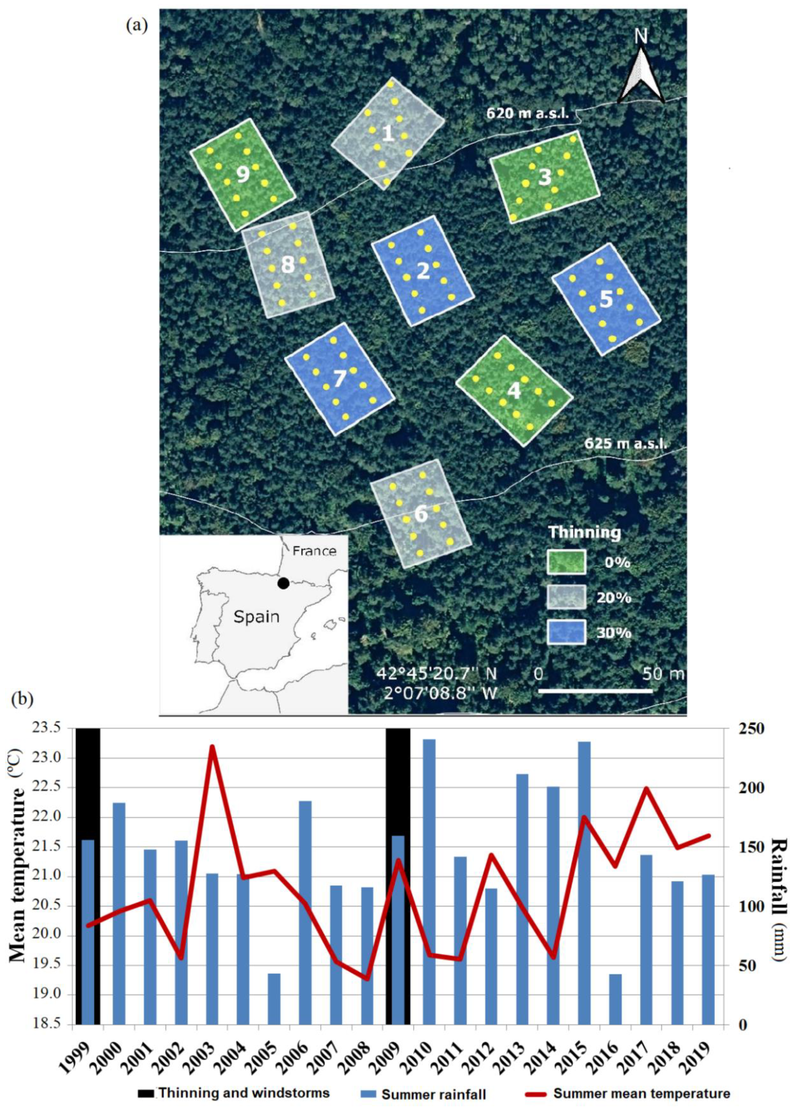
2.1. Study Area

The study site is a forested area located near the village of Aspurz (Navarre province, northeastern Spain), in a north-facing foothill of the Southwestern Pyrenees, at 610–635 m a.s.l. (Figure 1). The climate is sub-Mediterranean, transitional between temperate and Mediterranean climates. During the last 20 years, mean annual precipitation was 913 mm and mean annual temperature 11.9 °C (Navascués weather station [34]). There is a mild water deficit during the summer season (typically in July and August), and frequent frosts from winter to early spring.

At our study site, strong winds occurred from 22 to 25 January 2009, with winds from west to east surpassing 100 km h⁻¹ [35]. This caused uprooting and stem and branch breakage in a noticeable number of trees (mostly pines), which opened gaps unevenly distributed in the forest canopy of several study plots. However, the intensity of this event was not enough to cause a general stand-replacing event. In addition, drought events occurred in 2005, 2011, 2012, and 2016, when the amount of accumulated rain was noticeably lower than the other years (Figure 1).

The stand is a natural mixed forest of Pinus sylvestris L. (Scots pine) and Fagus sylvatica L. (European beech), regenerated after strip-like clear-cutting during the mid-1960s. Currently, although much less numerous than pine trees, many beech trees are co-dominant or dominant, and occupy, on average, 39.4% of the forest canopy (our 2008 survey, unpublished data). The other individuals of broadleaved species occur as early stages of the natural regeneration processes, with a few individuals arriving to the mid-stages of canopy strata (7.3% and 0.5% of the mixed forest canopy, respectively, 2008 survey, unpublished data).

2.2. Experimental Design and Tree and Recruit Samplings

In November 1999, the Servicio Forestal del Gobierno de Navarra established a thinning trial composed by 9 plots (30 × 40 m size) with three different thinning intensities (0%, 20%, and 30% of basal-area removed), removing mainly suppressed or intermediate trees, and some dominant or co-dominant trees with malformed stems. In March 2009 a second thinning was performed, mainly focused on removing subdominant or dominant trees, repeating the 20% intensity but increasing the highest thinning intensity from 30% to 40%. In both thinning treatments, only Scots pine trees were removed in the research plots and in a surrounding 5 m buffer zone around the plots to avoid edge effects. In each plot, two roughly rectilinear transects were established in April 2000. In each transect, five sampling points were established every 7 m and marked with a wooden stake, accounting for 90 permanent sampling points (Figure 1).

2.3. Image Acquisition and Hemispherical Photographs

During the period 2005–2019, we took HPs on a yearly basis (in July, except in September 2012) in all sampling points. Photos were taken with a Nikkon CoolPix 995 camera (Tokyo, Japan), at dawn with good weather conditions, trying to assure stable and similar sky conditions across plots and years [36,37]. Each HP was acquired at 1 m height. Low-hanging vegetation close to the camera was not altered unless directly blocking the lens. For each sampling point, topographical data (orientation, latitude, and latitude were recorded to ensure proper azimuth angle to calculate the solar pathway). Unfortunately, data for the year 2017 were not analyzed, since they were lost due to file corruption. In total 1260 HPs were analyzed (see examples in Figure S1, Supplementary Materials). Once acquired, we individually checked each HP in order to adjust the brightness to avoid mismatching between the fraction that corresponds to the sky and to vegetation [38]. For each HP, we additionally calculated the relative angle of rotation with the actual north bearing.

2.4. Light Variables from Hemispherical Pictures

For each HP, we computed different light metrics using Hemiphot software [38], running under the R statistical language, which included our own additional modifications to calculate sunflecks (see below). In our study site, the geographical location (i.e., altitude and latitude) of each sampling point did not significantly differ between HPs, and thus we assumed that errors resulting in light indexes were negligible at stand-level scale. Atmospheric parameters in our study site were measured using parameters by [37]: for clear days, the indirect site factor (ISF) was set as 0.1 and the global site factor (GSF) was set as 0.9. Details of calculations of light variables can be found in [38].

(a) Canopy openness (CanOpen) refers to the fraction of the visible sky in a given location. CanOpen gives an independent light characteristic, not influenced by the location or the proper alignment with respect to geographic north [38]. In our case, we divided the projection of the hemispheric photography into 90 concentric rings, each ring corresponding to a circular sphere segment in the sky hemisphere with an arc of 1 degree.

(b) Leaf area index (LAI) of vegetation is defined as the amount of leaf area per unit of ground area. We used an indirect calculation based on a method described by [39]. Five viewing angles were used: 7, 23, 38, 53, and 68 degrees. The gap fractions (T) around each viewing angle, in bands of 13°, were calculated with similar methods as total openness for the hemisphere.

(c) Direct light is obtained from the direct photosynthetic photon flux density (PPFD) and represents the amount of light that reaches the upper part of the forest canopy. It is assumed that if the Sun is not obstructed by the forest canopy, direct light is equal to that of above the canopy (i.e., PPFD reaches maximum values). This approach is simple and ignores cloudiness, twilight effects, and scattering of the light when entering through the forest canopy. In our case, we first calculated direct light for both above (DirectAbove) and below (DirectBelow) canopy levels of the day with the higher solar radiation (21 June). Below light accounts for the light that trespasses the canopy layers. At the same time, the amount of photosynthetic influx was also estimated for the whole year (DirectAbove.Yr, DirectBelow.Yr).

(d) Diffuse light is related to the diffuse PPFDs, and represents the amount of light scattered by the atmosphere. The amount of diffuse light on a horizontal surface can be estimated as being 15% of the amount of direct light added to the amount of direct light on that same area. Same as done for the direct light, diffuse light was calculated for both above (DiffAbove) and below (DiffBelow) canopy levels for 21 June. Similarly, the yearly amount of diffuse photosynthetic influx was also estimated (DiffAbove.Yr, DiffBelow.Yr).

(e) Sunflecks are intermittent periods of high photon flux density at the forest understories and lower canopies of trees, which significantly improve carbon gain in vegetation [40]. In our study, we defined a sunfleck as that event in which the direct light below the canopy was larger than zero. For each HP, we calculated the number of sunflecks for 21 June (N.Sunflecks). Finally, we calculated the longest duration of the sunflecks for each HP (Max.Sunflecks) as a measure of the strongest photon flux density potentially received.

For each of the light variables listed above, we computed the mean and standard deviation values for all sampling points at plot level (

Table 2. Average values of the light-related variables for the monitored period (2005–2019). Values show average ± standard error. Broadleaf subcanopy cover was measured in a 1.0 m radius area surrounding the sampling point and broadleaf subcanopy richness was measured in a 4.0 m radius area.

Plot	CanOpen %	LAI m2 m−2	Direct Below µmol m−2 s−1	Direct Below.Yr µmol m−2 s−1	Diff Below µmol m−2 s−1	Diff Below.Yr µmol m−2 s−1	N.Sunflecs Number	Max. Sunflecks Minutes	Canopy Cover %	Canopy Richness # Species
Control
Plot 3	14.5 ± 1.6	3.16 ± 0.11	11.67 ± 1.74	8.92 ± 1.18	050 ± 0.04	0.43 ± 0.04	16.60 ± 1.95	0.32 ± 0.06	0.67 ± 0.59	2.80 ± 0.73
Plot 4	14.4 ± 2.0	3.54 ± 0.15	11.51 ± 2.14	7.82 ± 1.33	0.46 ± 0.05	0.40 ± 0.05	14.03 ± 1.85	0.39 ± 0.11	0.64 ± 0.47	2.17 ± 1.09
Plot 9	16.5 ± 2.2	3.42 ± 0.19	12.78 ± 1.83	11.21 ± 1.45	0.51 ± 0.06	0.44 ± 0.05	18.54 ± 2.04	0.28 ± 0.04	0.33 ± 0.43	1.90 ± 1.11
average	15.1 ± 1.9	3.37 ± 0.15	11.99 ± 1.90	9.32 ± 1.32	0.49 ± 0.05	0.42 ± 0.04	16.39 ± 1.95	0.33 ± 0.07	0.55 ± 0.50	2.29 ± 0.98
Light thinning
Plot 1	17.2 ± 2.1	3.03 ± 0.14	13.99 ± 1.98	10.07 ± 1.44	0.57 ± 0.06	0.49 ± 0.05	20.05 ± 2.32	0.34 ± 0.05	0.50 ± 0.51	2.23 ± 1.19
Plot 6	15.6 ± 2.2	3.33 ± 0.17	11.07 ± 1.91	9.96 ± 1.34	0.51 ± 0.06	0.45 ± 0.05	15.28 ± 1.90	0.38 ± 0.10	0.56 ± 0.38	2.93 ± 1.22
Plot 8	16.0 ± 2.0	3.43 ± 0.19	12.47 ± 2.06	9.03 ± 1.35	0.49 ± 0.05	0.42 ± 0.05	17.54 ± 2.11	0.30 ± 0.05	0.55 ± 0.49	3.03 ± 1.10
average	16.3 ± 2.1	3.27 ± 0.17	12.51 ± 1.99	9.68 ± 1.38	0.52 ± 0.06	0.45 ± 0.05	17.62 ± 2.11	0.34 ± 0.06	0.54 ± 0.46	2.73 ± 1.17
Heavy thinning
Plot 2	18.4 ± 2.2	3.33 ± 0.17	12.72 ± 1.94	10.63 ± 1.47	0.57 ± 0.06	0.50 ± 0.05	18.36 ± 2.05	0.30 ± 0.05	0.64 ± 0.66	2.90 ± 1.82
Plot 5	15.3 ± 1.7	3.31 ± 0.13	10.59 ± 1.49	8.12 ± 1.08	0.48 ± 0.04	0.42 ± 0.04	15.92 ± 1.63	0.28 ± 0.05	0.62 ± 0.53	2.27 ± 1.10
Plot 7	16.3 ± 2.0	3.49 ± 0.16	12.47 ± 1.83	8.86 ± 1.38	0.51 ± 0.05	0.44 ± 0.05	17.37 ± 1.92	0.35 ± 0.07	0.51 ± 0.48	3.03 ± 1.22
average	16.7 ± 2.0	3.38 ± 0.15	11.93 ± 1.75	9.20 ± 1.31	0.52 ± 0.05	0.45 ± 0.05	17.22 ± 1.87	0.31 ± 0.05	0.59 ± 0.56	2.73 ± 1.38
Site average	16.0 ± 2.0	3.34 ± 0.16	12.14 ± 1.88	9.40 ± 1.34	0.51 ± 0.05	0.44 ± 0.05	17.08 ± 1.98	0.33 ± 0.06	0.56 ± 0.50	2.59 ± 1.17

). The number of pictures used per year were 90 (10 per plot), except in 2012 (49 pictures) and 2015 (82 pictures). For 2012 and 2015, all plots have at least three usable pictures available per plot, except plot 2 in 2012 (two pictures) and plot 8 in 2015 (zero pictures). In addition, most of the plots for those years had 9 or 10 pictures, especially in 2015. Hence, the influence of missing pictures due to technical difficulties was minimal, with only 4.76% of all data missing or not included in further calculations due to low quality.

2.5. Canopy Richness and Broadleaf Cover

In 2003, 2008, and 2016, we obtained data of the structure of the forest canopy by means of field surveys and projections of broadleaf canopy cover. In each plot, we mapped homogeneous canopy areas covered by each tree species other than Scots pine with at least one individual taller than 2.0 m. Finally, we digitized the field data using geographic information systems (GIS) software by converting the set of individual canopy areas to geospatial polygons. For more information about the sampling procedure, see [41].

HPs capture the projection of the surrounding vegetation by extreme wide angles, but it remains unclear the area covered beyond the image acquisition. Due to the uncertainty at which distance HPs best capture the above-surrounding forest canopy, we followed a multiscale approach with the aim to identify the area best describing the relationship between HPs and the forest canopy. We set concentric circular buffers around each permanent sampling plot with radii of 1.0, 2.0, 3.0, 4.0, and 5.0 m, which comprised circular areas of 3.14, 2.57, 28.27, 50.27, and 78.54 m², respectively (see examples in Figure S2, Supplementary Materials).

For each buffer zone and sampling point, we overlapped the maps of projected tree species canopies and we calculated the number of tree species present and the proportion of forest canopy covered by one or more broadleaf tree species. In order to avoid calculation error in large size buffers, those buffers that exceeded the plot size were cropped to fit the plot limits.

2.6. Data Analyses

2.6.1. Correlation between Light Variables and Data Filters

Before running statistical analysis, we performed preliminary tests aiming to avoid problems of normality and of non-independent variables. In order to obtain robust comparisons, we calculated average values of all the variables across all years. In other words, correlation values did not purely rely on one year but on the average effect occurring along our study years. This approach allowed us to filter variables avoiding the influence of a specific event that could have occurred during a single year, but rather on the average trends.

We applied the Wilcoxon test to check independence of variables, and the Pearson correlation test to detect collinearity between pairs of variables. In our case, we set 0.7 as a threshold value to account for high correlation between pairs of variables, and we thus retained those variables that had a pair-correlation of r < 0.7. In case of multiple matches, we retained those variables that showed fewer correlations. Overall, we retained CanOpen, LAI, DirectBelow.Yr, N.sunflecks, and Max.Sunflecks for further analyses (Table S1, Supplementary Materials).

2.6.2. Differences between Years and Plots in Light Variables

To test for differences in light variables between years, we used general linear mixed-effect models (GLMM) by means of the “stats” package using R v4.0.3 [42], which included each light variable as a response variable and year and plot as a fixed factor. We performed a repeated measures design, which included sampling point as a subject random factor. In order to perform multiple pairwise comparisons between years and plots, we performed a Tukey’s multiple comparison with Bonferroni’s correction for multiple tests by means of “emmeans” library using R v4.0.3 [43]. Non-significant pairwise contrasts (p > 0.05) were not shown.

2.6.3. Time-Series Analyses of Light Variables

To evaluate the time-dependent effects of the light variables along studied years we applied time-series analyses to determine if such temporal patterns are affected at short- or long-term periods. We applied the Ljung–Box test for independence to ensure that our series were stationary (Table S2, Supplementary Materials). Afterward, we applied analyses of partial autocorrelation functions (PACF) of the dependent variables or light indexes. A PACF explains how the value of a time lag or year (y) evolves when compared to its previous one (y − 1); thus, we can weigh the amount of influence on a year based on the following one [44]. If the PACF values are close to zero, we can assume that the data are independent of the temporal pattern, whereas if they are far from zero we can assume that the data are affected by previous time-dependent patterns. If the PACF value becomes too positive, the positive value of one observation increases the probability of having a positive value for another observation, whereas negative PACF values increase the probability of having a negative value afterward [44]. PACF analyses were performed with the “tseries” library in R [45].

For each sampling point and year, we calculated PACF values of light variables (i.e., CanOpen, LAI, DirectBelow.Yr, N.sunflecks, Max.Sunflecks) and we calculated the average and standard deviation values for each plot. For gap filling and non-available values (see above), we used the mean value of the whole time series in those, assuming that our time series followed a stationary trend (Figure S3, Supplementary Materials). To account for the elevated number of pairwise comparisons, we used a Bonferroni test to adjust the significance of variable changes in the multiple comparisons.

2.6.4. Relationships between Light Properties and Forest Canopy Composition

To evaluate the capacity of light variables to predict forest canopy structure, we applied GLMMs, seeking if dependent variables (i.e., canopy richness or cover) could be explained by independent variables (i.e., light variables, plot, and year). We additionally included the sampling point as a subject random factor, following a repeated measures design. Before GLMMs, we applied the Shapiro–Wilk test to check the normality of our dependent variables. Specifically, we fitted a Poisson distribution (numerical discrete) for richness and Gaussian distribution (numerical continuous) for canopy cover, following in both cases log–link functions. Then we generated GLMMs including two sets of models, with both canopy richness and cover as dependent variables, and we tested if they could be predicted by light variables (i.e., CanOpen, LAI, DirectBelowLight, DiffuseBelow, N.Sunflecks, Max.Sunfleckts, DirectBelow.Yr, and DiffuseBelow.Yr.) as independent linear predictors. In this case, to be more exhaustive in our search we included, in each model, the year (2003, 2008, and 2016) and the plot as independent variables. In addition, the interactions of the thinning and year with the other light variables were specified (see above). We did not assume continuous factors to have independent effects on dependent variables. In each model, we accounted the interactions of years and plot with the corresponding light variables. Analyses were done with the “lme4” library in R [46]. As there were no HPs available for 2003, the canopy cover and richness for that year were compared with light variables obtained from the HPs taken in 2005. We assumed that the time difference was short enough to ensure that canopy structural changes were kept at a minimum.

Following a multiscale approach (see above), we generated different sets of models with different combinations of dependent variables extracted for five circular areas of increasing radius around each sampling point of 1.0, 2.0, 3.0, 4.0, and 5.0 m, respectively. For each dependent variable and buffer area, multiple independent models were generated with all possible combinations of variables. We used Spearman’s correlation to test wheter canopy cover and richness were strongly correlated (r_s > 0.7) only at the smallest buffer (1.0 m radius) (Table S3, Supplementary Materials).

As a selection criterion for the “best model”, we used a criterion of complexity and fit of the model to the data [47,48,49] using Akaike’s information criterion (AIC). In our case, the selection of models was carried out using the “MuMIn” library and the “dredge” function in R [50]. For each dependent variable (i.e., light variables), we finally retained the model with the lowest AIC scores from the five areas or buffers.

3. Results

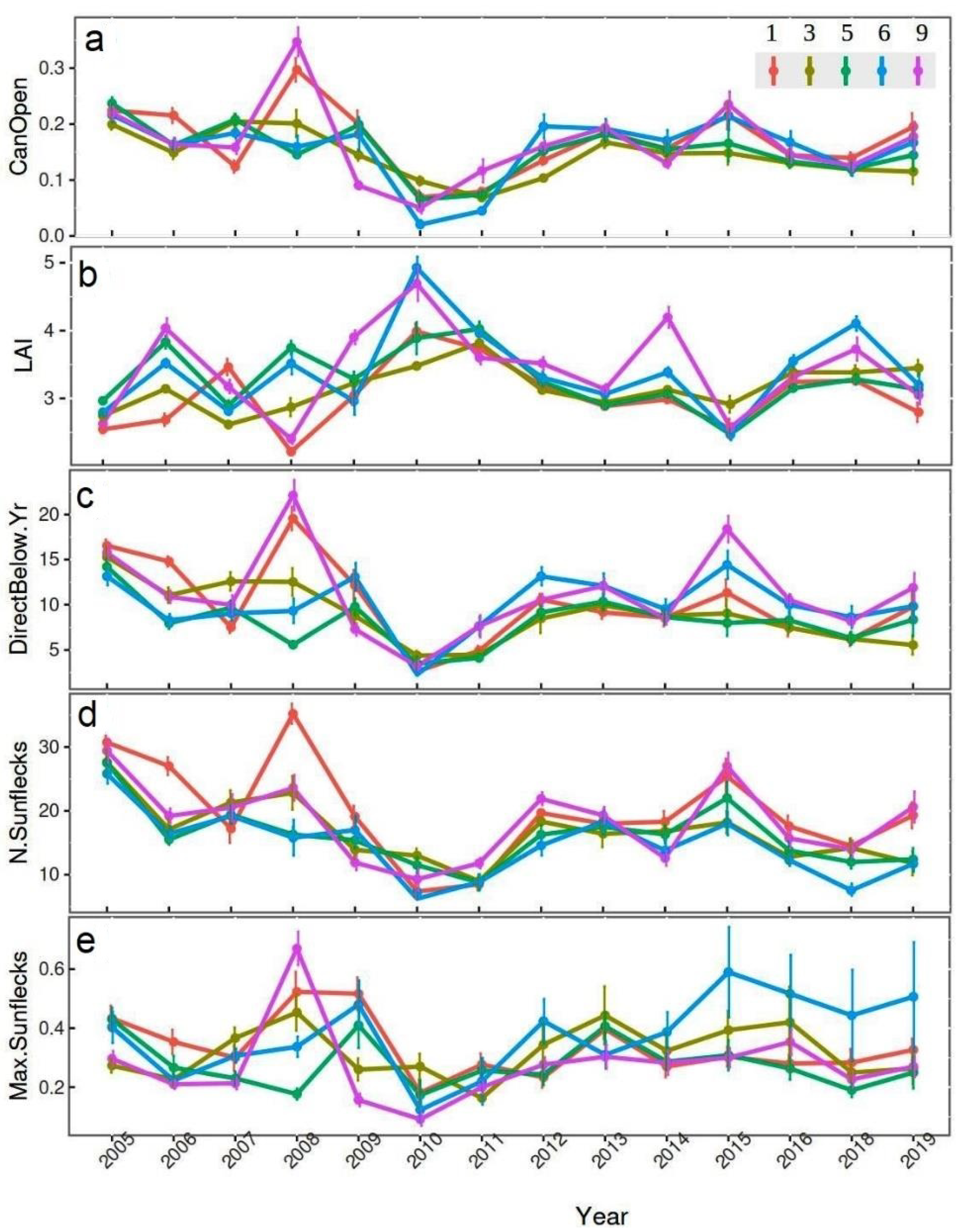
3.1. Temporal Changes in Light Variables

Overall, we found nonstationary trends of the values of light variables, with two major disturbance events occurring in 2010 and 2015 (Figure 2), and followed by recovery periods of the initial values recorded at the beginning of our time series. Maximum values in light variables were recorded prior to 2008, changing afterward to reach minimum values in 2010. This pattern was especially relevant for plot 1 (light thinning) and plot 9 (control), which were located in the north area of our study site. Light variables recovered their initial values in 2013. Afterward, we also detected a small increase of light values in 2015, with a subsequently fast recovery in 2016 (Figure 2). This event was especially strong for plot 6 (light thinning) and plot 9 (control). Regarding thinning treatments effects, they were not consistent over time, with the observed trends more dependent on peculiarities of each plot. Considering the whole monitored period, there was a trend to higher CanOpen in thinned plots, but not clear patterns for other variables (Table 2).

When taking into account the thinning treatments, for CanOpen (Figure 2a), the years with more significant contrasts were 2008 to 2010, followed by 2005–2006. For LAI (Figure 2b), the years with the most significant changes were 2015, 2009–2010, and 2005–2006. For DirectBelow.Yr (Figure 2c), significant contrast were found in 2008 to 2010 and 2015–2016. For N.Sunflecks (Figure 2d), the years appearing in the highest number of significant contrasts were 2005–2006, 2008–2009, and 2011. Finally, for Max.Sunflecks (Figure 2e) only a few years showed significant contrast in the period 2009 to 2011. Overall, we found a higher number of significant pairwise contrasts between plots, which suggests that the observed temporal patterns were more related to the intrinsic particularities to each plot than to thinning treatments (see Table S3, Supplementary Materials, for detailed results on pairwise contrast between consecutive years).

3.2. Spatial Differences in Light Variables

Regarding differences between plots within a single year, no clear patterns were found due to thinning treatments, being intrinsic plot-level features responsible for most of the observed differences among plots, with plot 1 and particularly plot 9 consistently showing light behaviors different from the other plots. In particular, for CanOpen plot 9 (a control plot) accumulated 29% of the significant differences among plots (pairwise contrasts) occurring from 2008 to 2010, followed by plot 6 (light thinning) and plot 7 (heavy thinning) with 14% and 11% of the significant differences among plots, respectively. For LAI, plot 1 (light thinning), plot 3 (control), and plot 9 (control) had 24.1%, 17.2%, and 13.8% of the significant differences, respectively, mainly from 2008 to 2010, and then 2014. For DirectBelow.Yr, again plot 9 accounted for 37.5% of the significant differences, mainly from 2007 to 2009. For N.Sunflecks, plot 1 and plot 9 accounted for 43.3% and 16.7% significant differences, respectively, mostly occurring in 2008 and 2009. Finally, the only significant pairwise contrast in Max.Sufnlecks was found for plot 9 (see results by thinning treatment in Figures S4–S6, Supplementary Materials).

Regarding differences between consecutive years among plots, the years with more significant contrasts for CanOpen were 2007 to 2010. For LAI, the years were 2008 to 2010 and 2014–2015; for DirectBelow.Yr, the years that account for most of the contrasts were 2007 to 2010, and then 2015. Finally, for Max.Sunflecks, only a few years showed significant contrast in the period 2009 to 2011. Overall, we found a higher number of significant pairwise contrasts between plots, which suggests that the observed temporal patterns were more related to intrinsic plot features than to thinning treatments (see Table S3, Supplementary Materials, for detailed results on pairwise contrast between consecutive years).

For both thinning treatments and plots, univariate models including plots as fixed factors explained a higher amount of variability (i.e., residuals or error terms having lower values), when compared to fitted models including thinning treatments as fixed factors. This pattern was consistent for all light variables (for model details, see Tables S5–S9 in Supplementary Materials).

3.3. Time-Dependent Effects on Light Variables

Exploring the time-dependent effects on light variable changes using partial autocorrelation functions (PACFs), we found strong changes, especially from 2005 to 2007 and from 2011 to 2012 for all the light variables (Figure 3). As when exploring temporal differences using the raw data of light variables, we did not find clear trends associated to thinning treatments, but the trends were more associated to intrinsic plot features (see results by thinning treatment in Figures S7–S9 in Supplementary Materials).

Comparing differences between light variables along studied years, we found that when taking the thinning treatment into account, CanOpen (Figure 3a) showed significant pairwise contrasts between consecutive years for the periods 2005–2007 and 2011–2012. For LAI (Figure 3b), significant contrasts were found for the period 2005–2007, and in 2011. For DirectBelow.Yr (Figure 3c) the significant contrasts were found in 2005–2006 and 2010 to 2012. For N.Sunflecks (Figure 3d) there were significant contrasts between consecutive years in the period 2005 to 2008, and in 2012. Finally, for Max.Sunflecks (Figure 3e), significant differences among consecutive years were found only for the period 2005 to 2008.

When taking into account differences between plots, a higher number of significant changes between consecutive years were found for all variables except N.Sunflecks. For CanOpen, significant pairwise contrasts were concentrated in 2005–2006, 2009 and 2011–2012. For LAI, changes were found in 2005 to 2009. For DirectBelow.Yr, significant contrasts between consecutive years were found for 2005–2007 and 2011–2012. For N.Sunflecks, the only significant contrast was found in 2005–2006. For Max.Sunflecks, significant contrasts were found in the period 2005–2007 (see Table S4, Supplementary Materials, for detailed results on significant pairwise contrast between consecutive years).

3.4. Forest Canopy Structure as Driver of Light Variables

When accounting for light variables explained by forest canopy variables, we found that an area of 4.0 m radius around each sampling point had the highest performance for CanOpen, DirectBelowYr, N.Sunflecks, and Max.Sunflecks, whereas an area of 2.0 m radius had the highest performance for LAI (see Figure S10, Supplementary Materials). When evaluating the best models to explain each light variable, the proportion of broadleaf canopy cover negatively affected the majority of the light variables (except for N.Sunflecks, which occurred in the best model, but it was not significant), whereas canopy richness only explained DirectBelow.Yr positively (

Table 3. Summary of the estimates for the “best model” accounting for the effect years, richness, and proportion of forest cover at explaining light variables, according to the AIC value, computed for an area of 5.0 m radius around each sampling point. Only the most significant values representing interactions between year, canopy richness, and proportion of forest cover are shown. Significant values (p < 0.05) are in bold.

Variables	Estimate	Std. Error	df	t Value	p Value
CanOpen
(Intercept)	0.265	0.009	210.796	29.453	0.000
PropCov	−0.110	0.014	149.936	−7.824	0.000
Year2008	0.027	0.009	189.448	2.835	0.005
Year2016	−0.032	0.011	252.260	−2.828	0.005
LAI
(Intercept)	2.865	0.096	12.183	29.972	0.000
PropCov	−0.296	0.060	259.631	−4.953	0.000
Year2008	0.255	0.064	258.033	4.016	0.000
Year2016	0.824	0.068	258.261	12.035	0.000
DirectBelow.Yr
(Intercept)	14.689	1.164	47.474	12.623	0.000
PropCov	−3.670	1.834	252.590	−2.001	0.047
Richness	0.653	0.275	232.342	2.379	0.018
Year2008	0.462	1.211	184.759	0.382	0.703
Year2016	−5.843	1.463	217.527	−3.995	0.000
PropCov:Year2008	−1.899	2.202	183.835	−0.863	0.390
PropCov:Year2016	0.556	2.130	204.093	0.261	0.794
N.Sunflecks
(Intercept)	30.477	2.083	92.589	14.629	0.000
PropCov	−3.532	2.656	253.321	−1.330	0.185
Richness	−0.859	0.763	255.344	−1.126	0.261
Year2008	−3.787	2.461	191.487	−1.539	0.125
Year2016	−17.027	2.848	208.860	−5.979	0.000
PropCov:Year2008	−7.120	3.384	185.216	−2.104	0.037
PropCov:Year2016	1.229	3.210	203.560	0.383	0.702
Richness:Year2008	1.787	0.939	204.944	1.904	0.058
Richness:Year2016	1.764	0.895	223.855	1.971	0.050
Max. Sunflecks
(Intercept)	0.467	0.033	152.423	14.319	0.000
PropCov	−0.132	0.047	195.165	−2.804	0.006

). In addition, we found that the effect of broadleaf canopy cover and richness at explaining light variables covaried with years, but only in N.Sunflecks. In particular, we found a negative effect of broadleaf canopy cover in 2008, whereas a positive effect of canopy richness in 2016 (Table 3).

4. Discussion

Overall, we found that the non stand-replacing windstorm in 2009 caused a strong signal in the properties of the light available for the understory, tending to recover two to three years after such event. Likewise, drought events (i.e., 2005 and 2012) generated moderate changes in the temporal trend of understory light properties, with a fast recovery time (typically along the subsequent year). Therefore, our first hypothesis can be accepted, corroborating similar canopy response to diffuse disturbances reported previously [51]. However, we did not find strong associations between thinning treatments and trends in light properties, suggesting that human-caused and natural disturbances can interact among them at tree-level scales, making difficult to particularize the effects of individual disturbances.

We also found that that the buffer area of 4.0 m radius around the sampling points was the one best explaining the majority of light variables. In addition, we found that the majority of light variables predicted the proportion of ground covered by the broadleaf subcanopy, whereas only a few of these light variables exolained the species richness of the broadleaf canopy. Hence, our second hypothesis can be accepted for canopy cover but not for canopy richness, indicating that species functional traits, rather than diversity, are influencing light levels in the understory.

4.1. Light Variables and Their Temporal Autocorrelation

Thinning and windstorms are two disturbances that commonly generate moderate gaps in forest canopy (through tree removal or breakage), which directly influence light availability in forest systems [52,53]. For the 14-year monitoring period, we found that the years with the strongest variation in light properties were 2009 and 2010. During these two years, the minimum values occurred for almost all light variables, except for LAI, which reached its maximum. At the same time, light properties recovered in 2–3 years after the 2009 events, following a stationary or stochastic pattern later on. The latter trend was confirmed with the values of the partial autocorrelation analysis, which reached the lowest values in 2009 and 2010, indicating the lowest dependence of values on previous years.

Regarding forest management, previous research has demonstrated the effect of thinning on light variables, particularly by increasing the light transmittance within the forest understory, leading to enhanced understory survival and growth [54,55]. However, in our study such effects were not detected, so we can assume that there may be additional factors affecting the within-plot variability of understory light properties, overriding potential changes caused by thinning. Given the coincidence in time of thinning and windstorms in the same year (2009), their individual effects could not be separated, but we found that changes in light properties varied inconsistently between thinning treatments and were more dependent on the temporal and spatial dynamics of each plot. In particular, we found that plot 1 (20% thinning), plot 3 (control) and, notably, plot 9 (also control) had strong differences in the light properties, probably due to their different stand structure compared to other plots at our study site (Table 1). All of those more-affected plots were located in the northern area of our study site (Figure 1). Given that this spatial pattern was independent on the thinning treatment, we could assume that the plot particularities, combined with the windstorm event, blurred the potential effect of thinning, and thus we had difficulty finding differences between thinning treatments. Furthermore, a study performed by [56] showed that considering slopes when studying light properties with HP could be useful to better predict the effect of natural disturbances on a particular forest patch. Our results also reinforce Kramer et al.’s [57] conclusion that site factors are more important than management for canopy performance and recovery during disturbances. In spite of this, as thinning is being increasingly suggested as a management practice to adapt forest stands in drought-prone areas to increasingly reduced water availability by reducing evapotranspiration [58,59], it could be interesting to repeat the thinning experiments without the influence of windthrow to better characterize its influence on understory light.

On the other hand, it has been assumed that windstorms could be a key abiotic factor that generate gaps in forest ecosystems [60,61], a pattern consistent with our findings. Strong winds affect forest dynamics by causing tree and branch mortality, and increasing woody debris, whereas thinning is usually followed by forest floor cleaning, which allows seedling regeneration [62]. However, we found that the lowest values of CanOpen, DirectBelow.Yr, and N.Sunflecks occurred in 2010 and 2011 (with LAI showing the opposite pattern), which were the years after thinning and strong winds had happened. Although this pattern could seem counterintuitive at first glance, we suggest that the combination of thinning and strong winds allowed greater light availability at the forest understory, triggering the growth of subcanopy and understory species (such as Rubus spp. or Pteridium aquilinum L, or saplings of broadleaves, abundant in our study site), consequently increasing LAI values and growing above 1 m (i.e., the height at which HP were taken) [51,62]. In particular, [63] demonstrated that LAI values in shrub-dominated zones were higher compared to tree-dominated zones, eventually implying that abandonment of forest management practices led to a decrease in both the availability and the spatial heterogeneity of understory light due to tree canopy expansion. After such events, the forest canopy is covered by trees and tall shrubs in the understory (such as Prunus spp., Quercus spp. in early regeneration stages, Buxus sempervirens L., etc.), lowering the values of CanOpen, DirectBelow.Yr, and N.Sunflecks. However, we found that the latter alteration was more localized than generalized, and only a small number of plots had strong changes in light properties (notably those located in the northern area of our study plot; see above), likely as a consequence of opening the tree canopy by branch and stem breakage and some tree uprooting by strong wind storms.

As an additional factor, drought has direct impacts on health, dynamics, and abundance of tree species [9]. During the short-term, drought triggers overstory defoliation and leads to increased light availability for the understory [64], a pattern that is additionally modulated by the species-specific responses to stress. For the mid- to long-term, severe droughts can produce important reductions in tree growth or eventual deaths [65,66]. In our study site, we detected changes in light properties during 2006 and from 2012 to 2014, likely derived from drought events occurring during those particular years [67]. Compared to the 2009 thinning plus windstorm event, droughts generated more moderate changes in light variables, but still noticeable, particularly in CanOpen, LAI, DirectBelow.Yr, and N.Sunflecks. Unfortunately, we could not carry out a detailed plot-level analysis of drought effects as we lacked direct soil moisture measurements during the monitoring period.

These events led to increases in available light at the forest understory (i.e., higher values for CanOpen, DirectBelow.Yr, and N.Sunflecks and lower values of LAI), probably as a consequence of defoliation. At this site, a positive relationship between increased litterfall production and summer droughts has been reported [8], and P. sylvestris and F. sylvatica leaf litterfall production has been linked to climatic changes [68]. The composition of overstory tree species, the abundance and vertical distribution of understory vegetation, and the soil type (through its influence on vegetation) are also crucial in factors influencing understory light properties [69]. At our site, defoliation due to summer drought was quickly recovered the following year [8], supporting our finding that light properties were quickly recovered after the drought events. This fact suggests that tree vitality at this site is enough to cope with isolated drought events [70]. As occurred with the strong wind event in January 2009, the drought events seem to have affected only some plots.

Finally, for the same forest and time period, [68] reported a strong increase in broadleaf production over time, shifting leaf litter from being pine-dominated in 2000 to beech-dominated by 2017. This change in the canopy biomass composition could be related with a certain gradual understory shadowing over the 14-year time period, as shown by the lower light levels measured in the later years when compared to the initial years. This can be interpreted as a signal of forest succession within the stationary series, as once the forest canopy regains its structure, the increasingly dominant broadleaf trees have stronger effects on the light conditions underneath, both decreasing understory LAI values and stabilizing other light variables.

4.2. Relationships between Forest Canopy Structure and Understory Light Variables

We found a strong influence of the size of the area around each sampling point when explaining light variables by forest structure factors (cover and richness). Our findings suggested that a radius of 4.0 m (~50 m²) was the most suitable. This fine spatial scale (small patch, almost tree-level) suggests that forest structure directly above the sampling point explained most of the light properties in the understory. This is directly linked to the presence of beech, which dominates the light environment in the subcanopy and understory layers. As demonstrated by [71,72], beech has greater leaf area per tree compared to other species such as Acer pseudoplatanus L. (maple), Fraxinus excelsior L. (ash), or Quercus pubescens (oak), which are also present in our study site. However, we should note that the canopy covered by pine was not included in the analysis, as it was assumed to be a homogeneous distribution (based on stem distribution maps) on the top canopy layer (~20 m), above all the broadleaves, which were considered as the species that actually created the heterogeneity in the canopy structure. However, this assumption may have caused a bias for the first years in the series, when the dominance of pine over the broadleaves was more clear [68].

In addition, we also found that species richness was able to explain certain light properties, particularly DirectBelow.Yr and N.Sunflecks. Morin et al. [73] reported that higher species richness leads to a larger leaf area index because of higher diversity in leaf traits. In our study site, species richness is directly related to the presence of shade-tolerant woody species. Diffuse light (dominated by overstory layer), species richness, beech proportion in the overstory, and heterogeneity of tree diameters have been described as the most important drivers of species composition [60]. In our case, DirectBelow.Yr was positively related to species richness, whereas N.Sunflecks showed a negative relationship, as more leaf traits were translated into a more dense cover, reducing the possibility of direct light reaching the understory layer.

Our findings suggest that a fine spatial scale at patch-level (4.0 m radius or ~50 m²) allows for including the presence of non-dominant broadleaf trees, which are more heterogeneously distributed than the pine overstory and that have been proven as important in defining the understory light environment. Although we did not study the effects of individual tree species on light variables, species richness can be considered a proxy of canopy complexity [74]. Higher species richness resulted in increased space filling in the shadowed lower canopy levels in mixed forests [75]. Hence, tree species diversity positively affected canopy complexity [76]. Based on our results, we suggest that it is necessary to consider the entire tree species composition when studying the understory light environment, as relying purely on light properties of the dominant species could provide biased information.

4.3. Management Implications

To date, thinning in this mixedwood has focused only on Scots pine, leaving beech unmanaged [41]. Consequently, beech growth has been favored through recruitment of new individuals and important crown expansion of the trees already present, a situation representative of most of the pine forests in the Pyrenees. Even if Scots pine still is the dominant species at this site, this situation will soon change as beech is a very competitive species and small light gaps are enough for it to grow taller. This will likely result in a darker and more homogeneous understory light environment, which could also be less prone to the changes caused by windstorms, as broadleaves significantly reduce vulnerability to wind when admixed with conifer species [77], resulting in increased temporal stability. However, if drought events worsen in a future with warmer climate [28], thinning could focus on beech individuals as a way to reduce the increased shadow on the understory. Even if beech canopy could be less influenced by droughts because this species’ characteristic leaf development [78], removing some beech trees could help other less shade-tolerant species such as maple or ash to develop better [72], thus maintaining forest mosaics and enhancing biodiversity, which is important for light properties, as seen in our study. Thinning could also help other Mediterranean species better adapted to drought conditions, such as the pine itself or oaks to develop, while decreasing competitiveness of the beech, and maintaining biodiversity (compared to pure stands of beech or pine). Overall, long-term monitoring of canopy structure development and understory light conditions will remain important in the future to better understand the relationship between moderate but frequent natural and anthropogenic disturbances during the ecological succession from conifer to broadleaves, particularly under the uncertainty of future climate change.

5. Conclusions

As forest management moves towards the paradigm of near-nature forestry, a better understanding on how disturbances affect light (one of the main growth limiting factors for the understory) is needed. All things considered, we found that this mixed conifer–broadleaf Mediterranean forest quickly recovered from abiotic (windstorms and drought) and anthropogenic disturbances (thinning) after two to three years, suggesting stability and resilience of this mixedwood to environmental changes. Our results also indicated the importance of non stand-replacing disturbances such as winds, thinning, and droughts as the main drivers affecting changes in the understory light environment. Our findings also suggest that canopy cover is the main structural feature influencing understory light properties, but species richness also adds important information to better understand light variability in the forest understory.

Last but not least, our study highlights the feasibility of using HP to keep track of how light parameters change within the forest, and what these changes explain. As we have already accumulated 14 years of data, we are encouraged to keeping using this methodology as a practical tool for long-term monitoring and research programs, making possible further comparison of new data with the data retrieved here. Finally, because hemispherical photographs can be improved, for instance, with new smartphone devices [79], HP can potentially become even easier to conduct in the near future.

References

1. Mátyás, C. Forests and Climate Change in Eastern Europe and Central Asia; Food and Agriculture Organization of the United Nations (FAO): Rome, Italy, 2010; Volume 8. [Google Scholar]
2. Dale, V.L.; Joyce, L.A.; McNulty, S.; Neilson, R.P.; Ayres, M.P.; Flannigan, M.D.; Hanson, P.J.; Irland, L.C.; Lugo, A.E.; Peterson, C.J.; et al. Climate change and forest disturbances. Bioscience 2001, 59, 723–734. [Google Scholar] [CrossRef] [Green Version]
3. Dubrovskis, E.; Donis, J.; Racenis, E.; Kitenberga, M.; Jansons, A. Wind-induced stem breakage height effect on potentially recovered timber value: Case study of the Scots pine (Pinus sylvestris L.) in Latvia. For. Stud. 2018, 69, 24–32. [Google Scholar] [CrossRef] [Green Version]
4. Yamamoto, S.-I. Forest gap dynamics and tree regeneration. J. For. Res. 2000, 5, 223–229. [Google Scholar] [CrossRef]
5. Quine, C.P.; Gardiner, B.A. Understanding how the interaction of wind and trees results in windthrow, stem breakage, and canopy gap formation. In Plant Disturbance Ecology; Elsevier: Amsterdam, The Netherlands, 2007; pp. 103–155. [Google Scholar]
6. Ulanova, N.G. The effects of windthrow on forests at different spatial scales: A review. For. Ecol. Manag. 2000, 135, 155–167. [Google Scholar] [CrossRef]
7. Meng, S.X.; Rudnicki, M.; Lieffers, V.; Reid, D.E.B.; Silins, U. Preventing crown collisions increases the crown cover and leaf area of maturing lodgepole pine. J. Ecol. 2006, 94, 681–686. [Google Scholar] [CrossRef]
8. Blanco, J.A.; Imbert, J.B.; Castillo, F.J. Nutrient return via litterfall in two contrasting Pinus sylvestris forests in the Pyrenees under different thinning intensities. For. Ecol. Manag. 2008, 256, 1840–1852. [Google Scholar] [CrossRef]
9. Clark, J.S.; Iverson, L.; Woodall, C.W.; Allen, C.D.; Bell, D.; Bragg, D.C.; D’Amato, A.W.; Davis, F.; Hersh, M.; Ibanez, I.; et al. The impacts of increasing drought on forest dynamics, structure, and biodiversity in the United States. Glob. Chang. Biol. 2016, 22, 2329–2352. [Google Scholar] [CrossRef] [Green Version]
10. Spinoni, J.; Vogt, J.V.; Naumann, G.; Barbosa, P.; Dosio, A. Will drought events become more frequent and severe in Europe? Int. J. Climatol. 2017, 38, 1718–1736. [Google Scholar] [CrossRef] [Green Version]
11. Flower, C.E.; Gonzalez-Meler, M.A. Responses of temperate forest productivity to insect and pathogen disturbances. Ann. Rev. Plant Biol. 2015, 66, 547–569. [Google Scholar] [CrossRef]
12. Anaya-Romero, M.; Muñoz-Rojas, M.; Ibáñez, B.; Marañón, T. Evaluation of forest ecosystem services in Mediterranean areas. A regional case study in South Spain. Ecosyst. Serv. 2016, 20, 82–90. [Google Scholar] [CrossRef]
13. Oliver, C.D.; Larson, B.A. Forest Stand Dynamics; John Wiley & Sons: New York, NY, USA, 1996. [Google Scholar]
14. Côté, I.M.; Darling, E.; Brown, C. Interactions among ecosystem stressors and their importance in conservation. Proc. R. Soc. B Boil. Sci. 2016, 283, 20152592. [Google Scholar] [CrossRef] [PubMed]
15. Müller, F.; Baessler, C.; Schubert, H.; Klotz, S. Long-Term Ecological Research; Springer: Berlin/Heidelberg, Germany, 2010; pp. 978–990. [Google Scholar]
16. Lindenmayer, D.B.; Likens, G.E.; Andersen, A.; Bowman, D.; Bull, C.M.; Burns, E.; Dickman, C.R.; Hoffmann, A.A.; Keith, D.A.; Liddell, M.J.; et al. Value of long-term ecological studies. Austral. Ecol. 2012, 37, 745–757. [Google Scholar] [CrossRef]
17. Lieffers, V.J.; Messier, C.; Stadt, K.J.; Gendron, E.; Comeau, P.G. Predicting and managing light in the understory of boreal forests. Can. J. For. Res. 1999, 29, 796–811. [Google Scholar] [CrossRef]
18. Weiner, J. Asymmetric competition in plant populations. Trends Ecol. Evol. 1990, 5, 360–364. [Google Scholar] [CrossRef]
19. Modrý, M.; Hubený, D.; Rejšek, K. Differential response of naturally regenerated European shade tolerant tree species to soil type and light availability. For. Ecol. Manag. 2004, 188, 185–195. [Google Scholar] [CrossRef]
20. Berentsen, W.H.; East, W.G.; Poulsen, T.M.; Windley, B.F. Europe. Encyclopedia Britannica. 2020. Available online: https://www.britannica.com/place/Europe (accessed on 28 October 2021).
21. Tsai, H.-C.; Chiang, J.-M.; McEwan, R.W.; Lin, T.-C. Decadal effects of thinning on understory light environments and plant community structure in a subtropical forest. Ecosphere 2018, 9, e02464. [Google Scholar] [CrossRef] [Green Version]
22. Lelli, C.; Bruun, H.H.; Chiarucci, A.; Donati, D.; Frascaroli, F.; Fritz, Ö.; Heilmann-Clausen, J. Biodiversity response to forest structure and management: Comparing species richness, conservation relevant species and functional diversity as metrics in forest conservation. For. Ecol. Manag. 2019, 432, 707–717. [Google Scholar] [CrossRef]
23. Lhotka, J.M.; Loewenstein, E.F. Effect of midstory removal on understory light availability and the 2–year response of underplanted Cherrybark oak seedlings. South. J. Appl. For. 2009, 33, 171–177. [Google Scholar] [CrossRef] [Green Version]
24. Naaf, T.; Wulf, M. Effects of gap size, light and herbivory on the herb layer vegetation in European beech forest gaps. For. Ecol. Manag. 2007, 244, 141–149. [Google Scholar] [CrossRef]
25. Pretzsch, H.; Biber, P. Tree species mixing can increase maximum stand density. Can. J. For. Res. 2016, 46, 1179–1193. [Google Scholar] [CrossRef] [Green Version]
26. Pretzsch, H.; del Río, M.; Schütze, G.; Ammer, C.; Annighöfer, P.; Avdagic, A.; Barbeito, I.; Bielak, K.; Brazaitis, G.; Coll, L.; et al. Mixing of Scots pine (Pinus sylvestris L.) and European beech (Fagus sylvatica L.) enhances structural heterogeneity, and the effect increases with water availability. For. Ecol. Manag. 2016, 373, 149–166. [Google Scholar] [CrossRef] [Green Version]
27. Blanco-Castro, E.; Casado González, M.Á.; Costa Tenorio, M.; Escribano Bombín, R.; García Antón, M.; Génova Fuster, M.; Gómez Manzaneque, A.; Gómez Manzaneque, F.; Moreno Saiz, J.C.; Morla Juaristi, C.; et al. Los Bosques Ibéricos: Una Interpretación Geobotánica; Planeta: Barcelona, Spain, 1997. (In Spanish) [Google Scholar]
28. De Andrés, E.G.; Seely, B.; Blanco, J.A.; Imbert, J.B.; Lo, Y.-H.; Castillo, F.J. Increased complementarity in water-limited environments in Scots pine and European beech mixtures under climate change. Ecohydrology 2017, 10, e1810. [Google Scholar] [CrossRef] [Green Version]
29. González de Andrés, E.; Camarero, J.J.; Blanco, J.A.; Imbert, J.B.; Lo, Y.H.; Sangüesa-Barreda, G.; Castillo, F.J. Tree-to-tree competition in mixed European beech–Scots pine forests has different impacts on growth and water-use efficiency depending on site conditions. J. Ecol. 2018, 106, 59–75. [Google Scholar] [CrossRef] [Green Version]
30. Seidel, D.; Fleck, S.; Leuschner, C.; Hammett, T. Review of ground-based methods to measure the distribution of biomass in forest canopies. Ann. For. Sci. 2011, 68, 225–244. [Google Scholar] [CrossRef] [Green Version]
31. Fournier, R.A.; Hall, R.J. Hemispherical Photography in Forest Science: Theory, Methods, Applications; Springer: The Netherlands, 2017. [Google Scholar]
32. Chianucci, F.; Cutini, A. Digital hemispherical photography for estimating forest canopy properties: Current controversies and opportunities. Ifor. -Biogeosci. For. 2012, 5, 290–295. [Google Scholar] [CrossRef] [Green Version]
33. Jonckheere, I.; Fleck, S.; Nackaerts, K.; Muys, B.; Coppin, P.; Weiss, M.; Baret, F. Review of methods for in situ leaf area index determination: Part, I. Theories, sensors and hemispherical photography. Agric. For. Meteorol. 2004, 121, 19–35. [Google Scholar] [CrossRef]
34. Meteo-Navarra. Meteorología y Climatología de Navarra: Navascués. 2021. Available online: http://meteo.navarra.es/estaciones/estacion.cfm?IDestacion=178 (accessed on 9 June 2021). (In Spanish).
35. AEMET—Spanish Meteorological Agency. Ciclogenesis Explosiva Enero. 2009. Available online: http://www.aemet.es/en/noticias/2009/03/ciclogenesisexplosiva (accessed on 16 February 2021). (In Spanish).
36. Pozueta, F. Hacia un Modelo Conceptual de la Biodiversidad en un Bosque Mixto de Pino-Haya. Master’s Thesis, Universidad Pública de Navarra, Pamplona, Spain, 2014. (In Spanish). [Google Scholar]
37. García-Sancet, M.A. Influencia de los Parámetros de Dosel y Lumínicos Sobre la Regeneración de Pinus sylvestris L. En un Bosque Mixto con Tres Intensidades de Clara. Master’s Thesis, Universidad Pública de Navarra, Pamplona, Spain, 2017. (In Spanish). [Google Scholar]
38. Ter Steege, H. Hemiphot.R: Free R Scripts to Analyse Hemispherical Photographs for Canopy Openness, Leaf Area Index and Photosynthetic Active Radiation under Forest Canopies. Naturalis Biodiversity Center, Leiden, The Netherlands. Available online: https://github.com/naturalis/Hemiphot (accessed on 3 August 2021).
39. Welles, J.M.; Norman, J.M. Instrument for indirect measurement of canopy architecture. Agron. J. 1991, 83, 818–825. [Google Scholar] [CrossRef]
40. Chazdon, R.L. Sunflecks and their importance to forest understorey plants. Adv. Ecol. Res. 1988, 18, 1–63. [Google Scholar] [CrossRef]
41. Arozarena, I. Influencia de la Gestión Forestal en la Evolución del Dosel Arbóreo en un Rodal Mixto del Prepirineo Navarro en Aspurz. Master’s Thesis, Universidad Pública de Navarra, Pamplina, Spain, 2020. (In Spanish). [Google Scholar]
42. Venables, W.N.; Ripley, B.D. Package MASS. Available online: http://www.r-project.org (accessed on 17 October 2012).
43. Lenth, R. Estimated Marginal Means, Aka Least-Squares Means. 1.4.8; R Package. Available online: https://CRAN.R-project.org/package=emmeans (accessed on 28 October 2021).
44. Hyndman, R.J.; Athanasopoulos, G. Forecasting: Principles and Practice; OTexts: Melbourne, VI, Australia, 2018. [Google Scholar]
45. Trapletti, A.; Hornik, K. Tseries: Time Series Analysis and Computational Finance. R Package Version 0.10-48. Available online: https://cran.r-project.org/web/packages/tseries/index.html (accessed on 3 August 2021).
46. Douglas, B.; Maechler, M.; Bolker, B.; Walker, S. Fitting linear mixed-effects models using lme4. J. Stat. Softw. 2015, 67, 1–48. [Google Scholar]
47. Sakamoto, Y.; Ishiguro, M.; Kitagawa, G. Akaike Information Criterion Statistics; Reidel: Dordrecht, The Netherlands, 1986. [Google Scholar]
48. Hu, S. Akaike Information Criterion. 2007. Available online: http://citeseerx.ist.psu.edu/viewdoc/download?doi=10.1.1.353.4237&rep=rep1&type=pdf (accessed on 3 August 2021).
49. Vrieze, S.I. Model selection and psychological theory: A discussion of the differences between the Akaike information criterion (AIC) and the Bayesian information criterion (BIC). Psychol. Methods 2012, 17, 228–243. [Google Scholar] [CrossRef] [Green Version]
50. Barton, K. MuMIn: Multi-Model Inference. 2020. Available online: http://CRAN.R-project.org/package=MuMIn (accessed on 28 October 2021).
51. Costilow, K.; Knight, K.; Flower, C. Disturbance severity and canopy position control the radial growth response of maple trees (Acer spp.) in forests of northwest Ohio impacted by emerald ash borer (Agrilus planipennis). Ann. For. Sci. 2017, 74, 10. [Google Scholar] [CrossRef] [Green Version]
52. Poulson, T.L.; Platt, W.J. Gap light regimes influence canopy tree diversity. Ecology 1989, 70, 553–555. [Google Scholar] [CrossRef]
53. Jonckheere, I.; Muys, B.; Coppin, P. Allometry and evaluation of in situ optical LAI determination in Scots pine: A case study in Belgium. Tree Physiol. 2005, 25, 723–732. [Google Scholar] [CrossRef] [PubMed] [Green Version]
54. Montes, F.; Pita, P.; Rubio, A.; Canellas, I. Leaf area index estimation in mountain even-aged Pinus silvestris L. stands from hemispherical photographs. Agric. For. Meteorol. 2007, 145, 215–228. [Google Scholar] [CrossRef]
55. Davi, H.; Baret, F.; Huc, R.; Dufrêne, E. Effect of thinning on LAI variance in heterogeneous forests. For. Ecol. Manag. 2008, 256, 890–899. [Google Scholar] [CrossRef]
56. Aussenac, G. Interactions between forest stands and microclimate: Ecophysiological aspects and consequences for silviculture. Ann. For. Sci. 2000, 57, 287–301. [Google Scholar] [CrossRef]
57. Kramer, K.; Brang, P.; Bachofen, H.; Bugmann, H.; Wohlgemuth, T. Site factors are more important than salvage logging for tree regeneration after wind disturbance in Central European forests. For. Ecol. Manag. 2014, 331, 116–128. [Google Scholar] [CrossRef]
58. Rodríguez-Calcerrada, J.; Pérez-Ramos, I.M.; Ourcival, J.M.; Limousin, J.M.; Joffre, R.; Rambal, S. Is selective thinning an adequate practice for adapting Quercus ilex coppices to climate change? Ann. For. Sci. 2011, 68, 575–585. [Google Scholar] [CrossRef] [Green Version]
59. Tinya, F.; Márialigeti, S.; Bidló, A.; Ódor, P. Environmental drivers of the forest regeneration in temperate mixed forests. For. Ecol. Manag. 2019, 433, 720–728. [Google Scholar] [CrossRef] [Green Version]
60. Schelhaas, M.-J.; Nabuurs, G.-J.; Schuck, A. Natural disturbances in the European forests in the 19th and 20th centuries. Glob. Chang. Biol. 2003, 9, 1620–1633. [Google Scholar] [CrossRef]
61. Lain, E.J.; Haney, A.; Burris, J.M.; Burton, J. Response of vegetation and birds to severe wind disturbance and salvage logging in a southern boreal forest. For. Ecol. Manag. 2008, 256, 863–871. [Google Scholar] [CrossRef]
62. Bond-Lamberty, B.; Fisk, J.P.; Holm, J.A.; Bailey, V.; Bohrer, G.; Gough, C.M. Moderate forest disturbance as a stringent test for gap and big-leaf models. Biogeosciences 2015, 12, 513–526. [Google Scholar] [CrossRef] [Green Version]
63. Valladares, F.; Guzmán, B. Canopy structure and spatial heterogeneity of understory light in an abandoned Holm oak woodland. Ann. For. Sci. 2006, 63, 749–761. [Google Scholar] [CrossRef] [Green Version]
64. Bréda, N.; Huc, R.; Granier, A.; Dreyer, E. Temperate forest trees and stands under severe drought: A review of ecophysiological responses, adaptation processes and long-term consequences. Ann. For. Sci. 2006, 63, 625–644. [Google Scholar] [CrossRef] [Green Version]
65. Bigler, C.; Bräker, O.U.; Bugmann, H.; Dobbertin, M.; Rigling, A. Drought as an inciting mortality factor in Scots pine stands of the Valais, Switzerland. Ecosystems 2006, 9, 330–343. [Google Scholar] [CrossRef] [Green Version]
66. Rubio-Cuadrado, Á.; Camarero, J.J.; del Río, M.; Sánchez-González, M.; Ruiz-Peinado, R.; Bravo-Oviedo, A.; Gil, L.; Montes, F. Long-term impacts of drought on growth and forest dynamics in a temperate beech-oak-birch forest. Agric. For. Meteorol. 2018, 259, 48–59. [Google Scholar] [CrossRef] [Green Version]
67. Candel-Pérez, D.; Lo, Y.-H.; Blanco, J.A.; Chiu, C.-M.; Camarero, J.J.; de Andrés, E.G.; Imbert, J.B.; Castillo, F.J. Drought-induced changes in wood density are not prevented by thinning in Scots pine stands. Forests 2018, 9, 4. [Google Scholar] [CrossRef] [Green Version]
68. De Andrés, E.G.; Blanco, J.A.; Imbert, J.B.; Guan, B.T.; Lo, Y.; Castillo, F.J. ENSO and NAO affect long-term leaf litter dynamics and stoichiometry of Scots pine and European beech mixedwoods. Glob. Chang. Biol. 2019, 25, 3070–3090. [Google Scholar] [CrossRef] [PubMed]
69. Messier, C.; Parent, S.; Bergeron, Y. Effects of overstory and understory vegetation on the understory light environment in mixed boreal forests. J. Veg. Sci. 1998, 9, 511–520. [Google Scholar] [CrossRef]
70. Rohner, B.; Kumar, S.; Liechti, K.; Gessler, A.; Ferretti, M. Tree vitality indicators revealed a rapid response of beech forests to the 2018 drought. Ecol. Indic. 2021, 120, 106903. [Google Scholar] [CrossRef]
71. Petriţan, A.M.; von Lüpke, B.; Petriţan, I.C. Influence of light availability on growth, leaf morphology and plant architecture of beech (Fagus sylvatica L.), maple (Acer pseudoplatanus L.) and ash (Fraxinus excelsior L.) saplings. Eur. J. For. Res. 2009, 128, 61–74. [Google Scholar] [CrossRef] [Green Version]
72. Sevillano, I.; Short, I.; Grant, J.; O’Reilly, C. Effects of light availability on morphology, growth and biomass allocation of Fagus sylvatica and Quercus robur seedlings. For. Ecol. Manag. 2016, 374, 11–19. [Google Scholar] [CrossRef] [Green Version]
73. Morin, X.; Fahse, L.; Scherer-Lorenzen, M.; Bugmann, H. Tree species richness promotes productivity in temperate forests through strong complementarity between species. Ecol. Lett. 2011, 14, 1211–1219. [Google Scholar] [CrossRef]
74. Zimmermann, A.; Zimmermann, B. Requirements for throughfall monitoring: The roles of temporal scale and canopy complexity. Agric. For. Meteorol. 2014, 189–190, 125–139. [Google Scholar] [CrossRef]
75. Seidel, D.; Leuschner, C.; Scherber, C.; Beyer, F.; Wommelsdorf, T.; Cashman, M.; Fehrmann, L. The relationship between tree species richness, canopy space exploration and productivity in a temperate broad-leaf mixed forest. For. Ecol. Manag. 2013, 310, 366–374. [Google Scholar] [CrossRef]
76. Fotis, A.T.; Morin, T.H.; Fahey, R.T.; Hardiman, B.; Bohrer, G.; Curtis, P.S. Forest structure in space and time: Biotic and abiotic determinants of canopy complexity and their effects on net primary productivity. Agric. For. Meteorol. 2018, 250-251, 181–191. [Google Scholar] [CrossRef]
77. Schütz, J.-P.; Götz, M.; Schmid, W.; Mandallaz, D. Vulnerability of spruce (Picea abies) and beech (Fagus sylvatica) forest stands to storms and consequences for silviculture. Eur. J. For. Res. 2006, 125, 291–302. [Google Scholar] [CrossRef]
78. Leuschner, C.; Voß, S.; Foetzki, A.; Clases, Y. Variation in leaf area index and stand leaf mass of European beech across gradients of soil acidity and precipitation. Plant Ecol. 2006, 186, 247–258. [Google Scholar] [CrossRef]
79. Bianchi, S.; Cahalan, C.; Hale, S.; Gibbons, J.M. Rapid assessment of forest canopy and light regime using smartphone hemispherical photography. Ecol. Evol. 2017, 7, 10556–10566. [Google Scholar] [CrossRef] [Green Version]
Figure 1. (a) Site location showing the nine plots used in the study. Green plots indicate control plots (no thinning), blue plots indicate heavy thinning, and uncolored plots indicate light thinning (see main text for details). Yellow dots indicate the sampling points where hemispherical photographs were taken. (b) Accumulated summer precipitation (June to August) and average summer temperature for the years of the study period. Black bars indicate the years with major disturbances (thinning and windstorms).
Forests 12 01485 g001
Figure 3. Partial autocorrelation functions (PACFs) for light variables over the studied years for the five plots with the clearest trends. (a) CanOpen, (b) LAI, (c) DirectBelow.Yr, (d) N.Sunflecks, and (e) Max.Sunflecks. Each line represents different plots. The y-axis represents the values the PACF can take (from 1.0 to −1.0), and the x-axis represents the years. For y-axis, values close to zero (dashed lines) show that there was no temporal autocorrelation of the values of each light variable with respect to the previous year.
Forests 12 01485 g002
Figure 2. Light variables from the hemispherical photograaphs during the studied years for the five plots that showed larger changes over time: (a) CanOpen (parts per unit), (b) LAI (m2 m−2), (c) DirectBelow.Yr (µmol m−2 s−1), (d) N.Sunflecks (µmol m−2 s−1), and (e) Max.Sunflecks (minutes). Each line corresponds to different plots. For each light variable, horizontal lines represent the mean values whereas vertical lines symbolize standard error.
Forests 12 01485 g003