Surface Detection of Solid Wood Defects Based on SSD Improved with ResNet

Abstract

Due to the lack of forest resources in China and the low detection efficiency of wood surface defects, the output of solid wood panels is not high. Therefore, this paper proposes a method for detecting surface defects of solid wood panels based on a Single Shot MultiBox Detector algorithm (SSD) to detect typical wood surface defects. The wood panel images are acquired by an independently designed image acquisition system. The SSD model included the first five layers of the VGG16 network, the SSD feature mapping layer, the feature detection layer, and the Non-Maximum Suppression (NMS) module. We used TensorFlow to train the network and further improved it on the basis of the SSD network structure. As the basic network part of the improved SSD model, the deep residual network (ResNet) replaced the VGG network part of the original SSD network to optimize the input features of the regression and classification tasks of the predicted bounding box. The solid wood panels selected in this paper are Chinese fir and pine. The defects include live knots, dead knots, decay, mildew, cracks, and pinholes. A total of more than 5000 samples were collected, and the data set was expanded to 100,000 through data enhancement methods. After using the improved SSD model, the average detection accuracy of the defects we obtained was 89.7%, and the average detection time was 90 ms. Both the detection accuracy and the detection speed were improved.

1. Introduction

Wood products are environmentally friendly. The appearance and performance of the wood are good, and the economic value and artistic value are high. As of December 2019, the Chinese total forest area reached 220 million hectares, with a forest coverage rate of 22.96%. However, Chinese per capita forest is less than 1/6 of the world’s average, so it is of great importance to increase the wood output rate and reduce waste. This requires us to efficiently locate and classify wood defects and retain valuable wood [1].

Defects in wood affect the strength and texture of the wood and must be removed during processing. Traditional detection of solid wood panels adopts the method of manual marking identification and later processing. Since the 21st century, the wood industry has also been actively exploring intelligent processing technology. As one of the emerging technologies, image processing technology has been widely used in wood detection [2,3]. The image processing procedure is roughly as follows: (1) obtaining the raw data (usually by scanning) from the sensor [4,5]; (2) extracting features and patterns from the data [6,7]; (3) making a decision after analyzing the information [8,9]. Digital image processing technology can identify wood defects, but the actual detection process is complex. Image segmentation [10,11] and the feature extraction process are usually very difficult, since the natural texture of wood products is complex, and defect types are quite different. Therefore, it is difficult to ensure the detection speed and accuracy. The application of deep learning methods [12,13,14] can improve the detection precision of surface defects of solid wood panels and achieve better detection performance on the premise of reducing the time of image processing.

Zhang [15] combined PCA with compression sensing methods for wood defect detection and used the least square method to classify the characteristics of different types of defects. Xie [16] took dead knots, pole and live knots of wood as research subjects and conducted in-depth studies on wood image segmentation and pattern recognition methods. Peng [17] proposed a wood defect detection for a tree species identification method based on 3D laser scanning. The measurement error of defect surface area and volume was less than 5%. Wang [18] used a fuzzy pattern recognition method to detect the surface defect level of particleboards in motion and calculated the number of defects, defect area and damage degree. Pahlberg [19] used thermal cameras to detect cracks in parquet floors, with an average classification accuracy of 0.8. Yang [20] used a 3D laser sensor system to classify and identify surface defects of lumber and agri-crop straw-based panels by selecting insect holes and dents as detection objects and obtained the final classification accuracy of 94.67% after applying SVM. Badrinarayanan [21] proposed a full convolution neural network for pixel segmentation with good segmentation performance, while Guo [22] proposed a multi-focus image fusion method based on a full convolution network. In recent years, algorithms related to extreme learning machines and other methods have been constantly improved and widely applied in practice [23,24,25].

In this paper, the SSD model is improved with the deep residual network. The performance of the improved model is compared with the single SSD model. The results show that the network structure used in this paper can improve the detection accuracy of surface defects of solid wood panels on the premise of reducing image processing time.

2. Materials and Methods

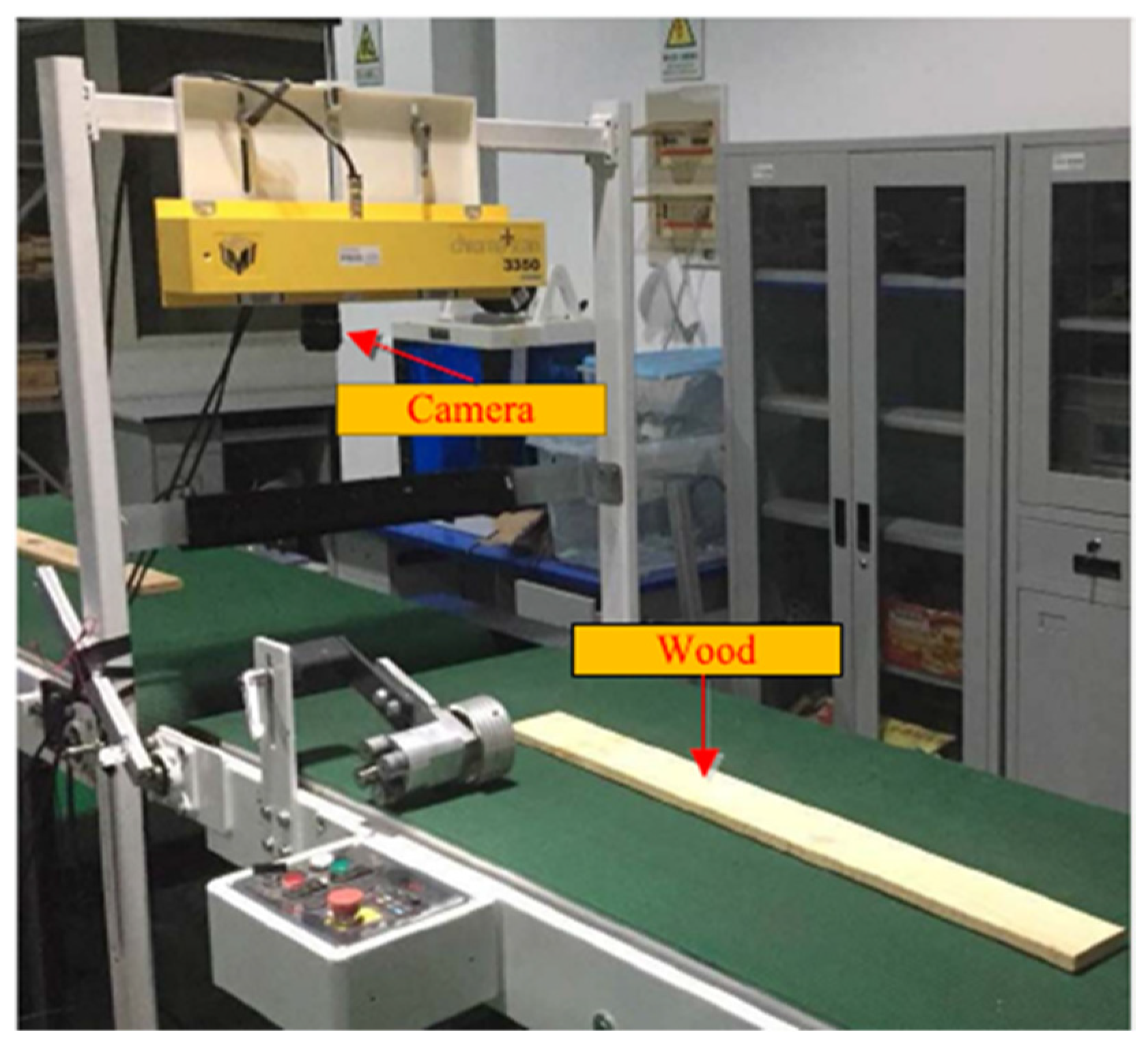
2.1. Image Acquisition and Environment Configuration

In this paper, the research object is the solid wood panel mainly made of Chinese fir and pine wood. We mainly detect the most representative defects such as knots, pinhole, crackle and decay on the surface of the solid wood panels. These defects will not only affect the appearance of the wood product but also cause the decrease in its physical and mechanical properties. The impact of several kinds of defects also varies with the type and the size of the defect. Worm holes with a diameter of less than 3 mm have a small effect on the performance of the wood and can be retained, but worm holes with a diameter of more than 5 mm need to be removed. The crack areas of the wood all need to be removed. Therefore, the judgment and treatment of the above defects are of great significance to the utilization of wood.

The image acquisition device for surface defects of solid wood panels set up in this paper is shown in Figure 1, which mainly includes a conveyor belt and linear CCD camera (LA-GC-02K05B, with a frequency of 1280 rows). Bar line light source (LCOL-300-25) is selected to provide a uniform light source. The transmission belt drives the solid wood panel to reach the illumination area at a uniform speed. The CCD industrial camera collects the surface image of the solid wood panel under the uniform illumination condition, and transmits the collected information to a PC for image processing.

Table 1. Software and hardware environment configuration table.

Hardware and Software	Name
System	Windows 10
CPU	Intel Xeon [email protected] GHz
Main panel	Dell 0X8DXD Core i7
Graphics card	Nvidia GeForce GTX 1080 Ti
Environment language	Python3.6/C++
Environment configuration	PyCharm + Visual Studio 2015
Deep learning framework	TensorFlow1.8.0

shows the hardware and software environment configuration adopted in this paper.

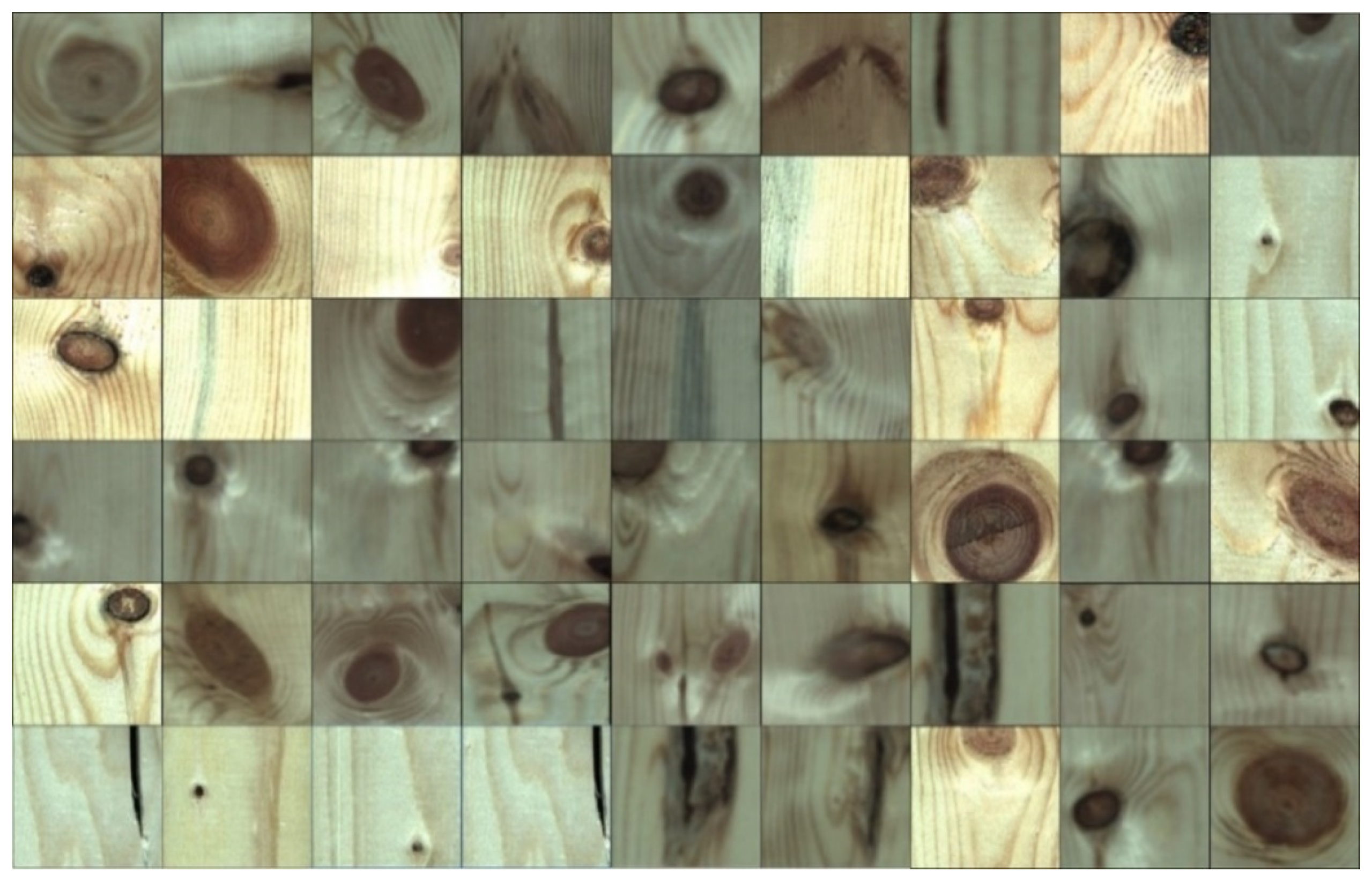
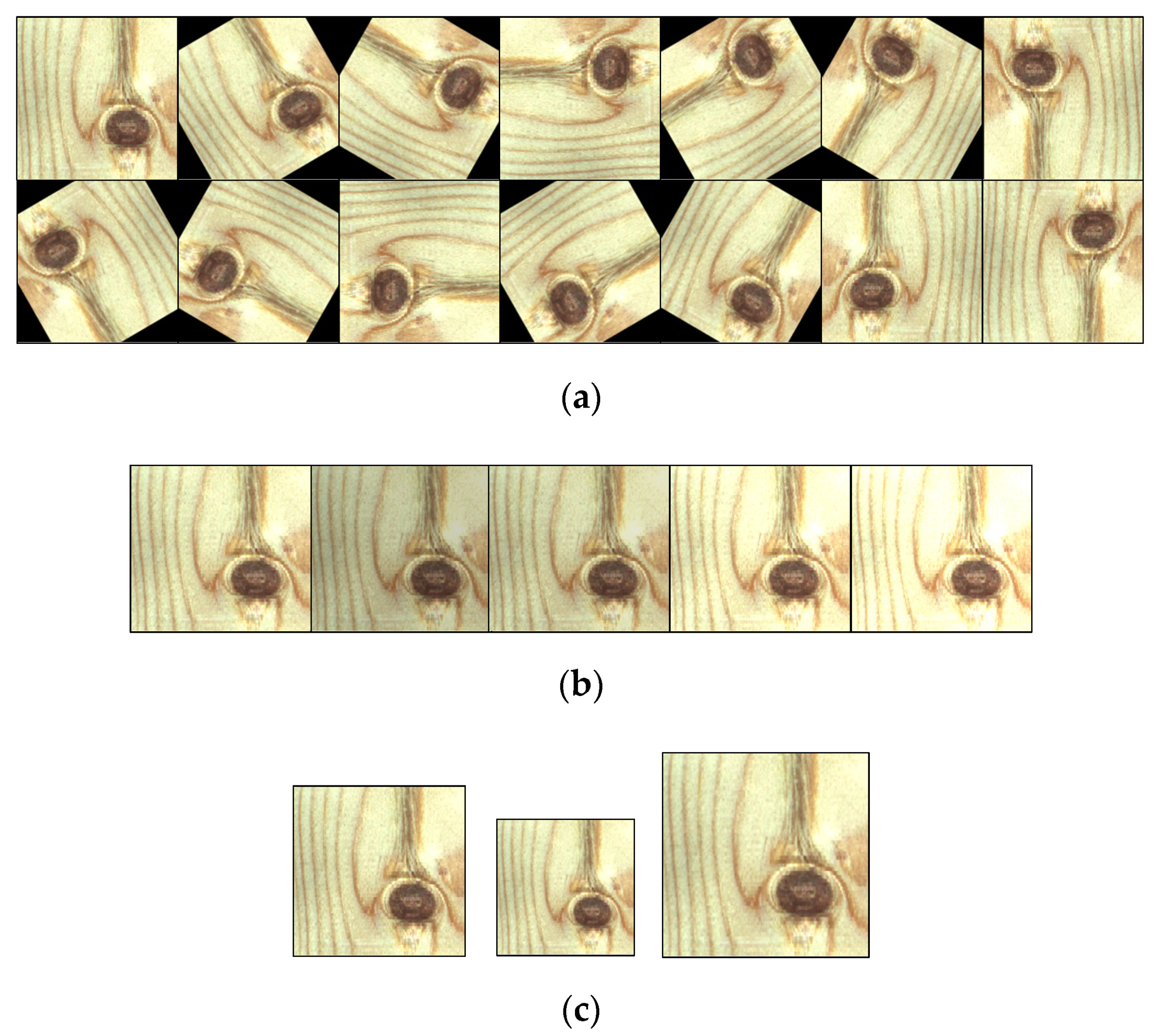
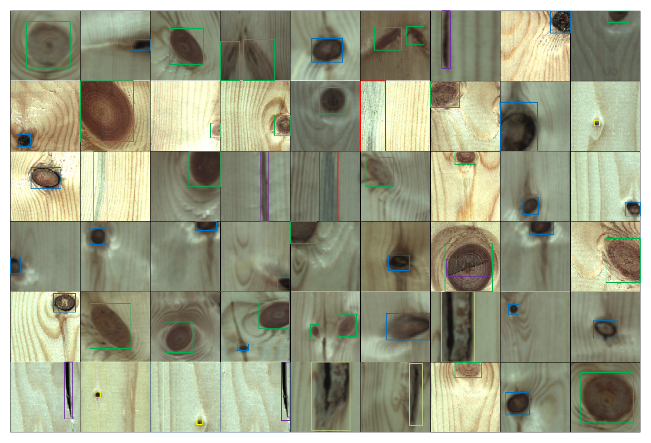
2.2. Establishment of Database

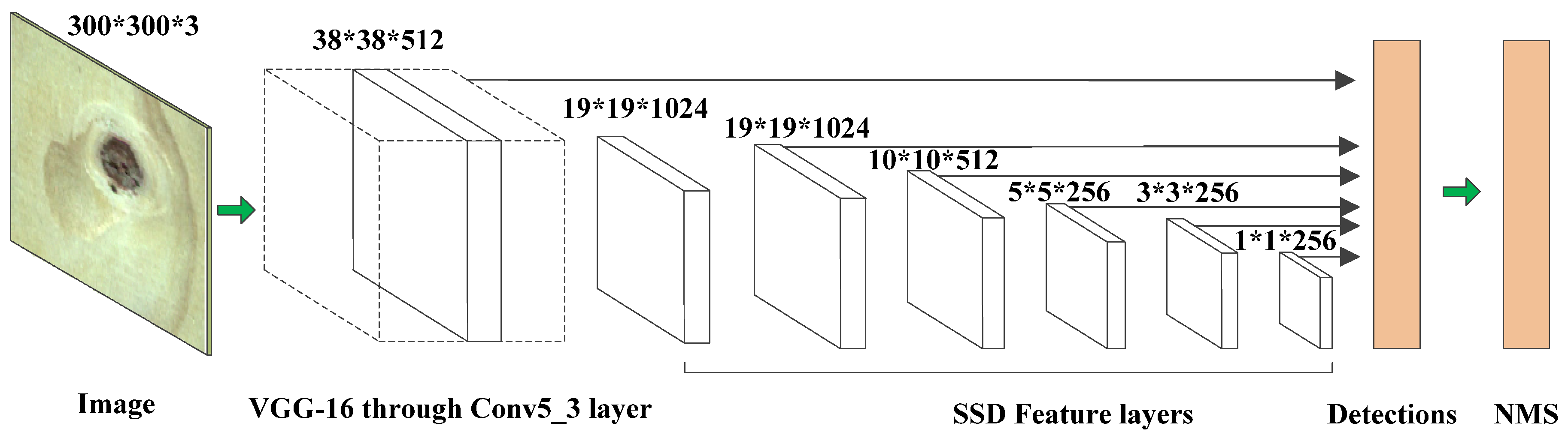
Using the image acquisition system in Figure 1, we have obtained more than 5000 pieces of 300 × 300 pictures of solid wood panels with defects. These defects mainly include six characteristic defects such as dead-knot, live-knot, decay, mildew, crackle, and pinhole. Parts of the sample images collected are shown in Figure 2.

In order to enrich the sample data, data enhancement has been carried out on the sample pictures, which have been obtained to meet the requirements of network training and avoid overfitting. According to the characteristics of solid wood panel images, the data enhancement process is implemented in the following three ways: (1) on the basis of ensuring the invariability of rotation and tilt of defect images, rotate defect images by different angles, and mirror the image based on horizontal and vertical directions; (2) adjust the brightness and saturation of defect images to simulate images taken under different lighting conditions; (3) randomly scale the defect image, 0.8 and 1.2 scales were selected. Through data enhancement, the original data set is expanded by 20 times so that the training sample data reaches more than 100,000 pieces. As shown in Figure 3, the defect image data of a solid wood panel is expanded. Then the obtained sample pictures are manually labeled. Parts of the labeled pictures are shown in Figure 4.

2.3. SSD Model

Liu [26] proposed an SSD network algorithm. The basic network of the SSD network model is VGGNet (Visual Geometry Group) [27]. The SSD model constructed in this paper includes the first five layers of the VGG16 network, an SSD feature mapping layer, a feature detection layer and NMS (non-maximum suppression) module, as shown in Figure 5. The first five layers of the VGG16 network are used for feature extraction. The SSD feature mapping layers are composed of a multi-layer convolutional neural network. The SSD feature mapping layers are used to map the default border score and the default border bias information. The feature detection layer can map all prediction results. The NMS module can process all the predicted results and finally output the prediction results of the detection.

2.4. General Procedure of SSD Algorithm

Given an input image and its truth value label, the processing flow of the SSD algorithm is as follows: (1) the input image is convolved in a series of CNN layers to obtain a certain number of feature graphs with different sizes (for example, 10 × 10, 6 × 6, 3 × 3); (2) The convolution filter of 3 × 3 is used to evaluate the default bounding box of target location in each feature graph. These default bounding boxes refer to the anchor mechanism of the Faster R-CNN algorithm. (3) Forecast the position offset and classification accuracy of each bounding box; (4) network training; (5) NMS algorithm is used to match the correct bounding box; (6) output classification results and bounding boxes.

The NMS algorithm process is as follows: Firstly, calculate the area of all bounding boxes, sort and score them according to the order from large to small. Then, the size of the intersection region of the bounding box with the highest ranking and the second highest ranking in the current sorting is cyclically calculated, as well as the proportion of the intersection region in the total region of the two bounding boxes (IoU). Then, the threshold set beforehand is compared with the IoU. If the former is larger, the bounding box of the second highest one is removed; otherwise, the second highest bounding box is retained. Finally, the remaining bounding boxes are processed in turn as described above.

The SSD algorithm uses a multi-scale method to obtain multiple feature maps of different scales. In this paper, it is assumed that m-layer feature maps are used for model detection. Then the formula for calculating the default frame ratio of the first k feature map is as follows:

$$S_k=S_{min}+\frac{S_{max}-S_{min}}{m-1}\left(k-1\right), k\in \left(1,2,\cdots ,m\right)$$

(1)

where $S_{min}$ is the minimum ratio of the default bounding box to the input image,$S_{max}$ is the maximum ratio of the default bounding box to the input image. Under normal circumstances, $S_{min}$ is set to 0.2 and $S_{max}$ is set to 0.95.

The SSD algorithm references many anchors of the Box mechanism of the Faster R-CNN algorithm and sets multiple aspect ratios for the default border of the same feature. Generally, these aspect ratios $r$ are in the range of $\left\{1, 2, 3,\frac{1}{2},\frac{1}{3}\right\}$. Then the width of the bounding box $w_k^{\alpha }=S_k\sqrt{{\alpha }_r}$, and the length of the bounding box $h_k^{\alpha }=S_k/\sqrt{{\alpha }_r}$ can be calculated. Among them, when the aspect ratio r = 1, an additional bounding box $S_k^{\prime }=\sqrt{S_k{S}_{k+1}}$ is added. Six default bounding boxes are set with different aspect ratios. At the same time, the center position of the default bounding box is expressed as:

$$\left(\frac{a+0.5}{\left|f_k\right|},\frac{b+0.5}{\left|f_k\right|}\right)$$

(2)

where $\left|f_k\right|$ is the size of the first $k$ feature map, $a,b\in \left\{0, 1,\cdots ,\left|f_k-1\right|\right\}$, and the coordinates of the default bounding box are set in the range [0,1].

Mapping the default bounding box of the feature layer to the original image coordinates, there are:

$$x_{min}=\frac{c_x-\frac{w_b}{2}}{w_{feature}}{w}_{img}=\left(\frac{a+0.5}{\left|f_k\right|}-\frac{w_b}{2}\right)w_{img}$$

(3)

$$y_{min}=\frac{c_x-\frac{h_b}{2}}{h_{feature}}{h}_{img}=\left(\frac{a+0.5}{\left|f_k\right|}-\frac{h_b}{2}\right)h_{img}$$

(4)

$$x_{max}=\frac{c_x+\frac{w_b}{2}}{w_{feature}}{w}_{img}=\left(\frac{a+0.5}{\left|f_k\right|}+\frac{w_b}{2}\right)w_{img}$$

(5)

$$y_{max}=\frac{c_x+\frac{h_b}{2}}{h_{feature}}{h}_{img}=\left(\frac{a+0.5}{\left|f_k\right|}+\frac{h_b}{2}\right)h_{img}$$

(6)

where $c_x$ and $c_y$ represent the center coordinate values of the default bounding box of the feature layer,$w_b$ and $h_b$ represent the width and height values of the default bounding box of the feature layer, $w_{feature}$ and $h_{feature}$ represent the mapping of the original image width and height values on the feature map, $w_{img}$ and $h_{img}$ represent the width and height values of the original image, ($x_{min}, y_{max}, x_{min}, y_{max}$) is the coordinate of the four vertices of the default bounding box mapped on the original image.

2.5. Loss Function

In the SSD algorithm network, the default bounding box is trained to find the most consistent detection box. The target loss function is usually established to achieve the regression of the actual detection box position and target type. The target loss function is calculated by the weighted sum of confidence loss and position loss. The specific form of the target loss function is as follows:

$$\mathrm{L}\left(z,c,l,g\right)=\frac{1}{N}\left(L_{conf}\left(z,c\right)+\alpha L_{loc}\left(z,l,g\right)\right)$$

(7)

where N is the number of default bounding boxes that match the actual detection box, $L_{conf}\left(z,c\right)$ and $L_{loc}\left(z,l,g\right)$ are the confidence loss and position loss, respectively, $z$ is the matching result of the actual detection box and the default bounding box,$c$ and $l$ are the confidence and position confidence of the predicted target bounding box, respectively, $g$ is the position information of the predicted target bounding box, $\alpha$ is the weight between the confidence loss and the position loss, which is set to 1 in this paper.

In this paper, $L_{conf}\left(z,c\right)$ and $L_{loc}\left(z,l,g\right)$ are calculated using Smooth L1 Loss [28]. The calculation formula is as follows:

$$L_{conf}\left(z,c\right)=-{\displaystyle \sum }_{i,j,p}{x}_{ij}^p\log \left(c_i^p\right)-{\displaystyle \sum }_{i,p}\left(1-{\displaystyle \sum }_{j,q=p}{x}_{ij}^p\right)\log \left(1-c_i^p\right)$$

(8)

$$L_{loc}\left(z,l,g\right)=\frac{1}{2}{\displaystyle \sum }_{i,j}{x}_{ij}^p||l_i-g_j^p{||}_2^2$$

(9)

where $x_{ij}^p$ is the first $j$ actual detection frame matched by the first $i$ default bounding box of category $p$ to which the target belongs.

The SSD algorithm combines the fast detection speed of the YOLO algorithm and the high detection accuracy of the Faster-CNN algorithm. It eliminates the full connection layer that consumes a lot of computing resources in the YOLO algorithm. Meanwhile, multi-scale feature maps are mapped on the detections layer to cover target categories of different sizes in the input images.

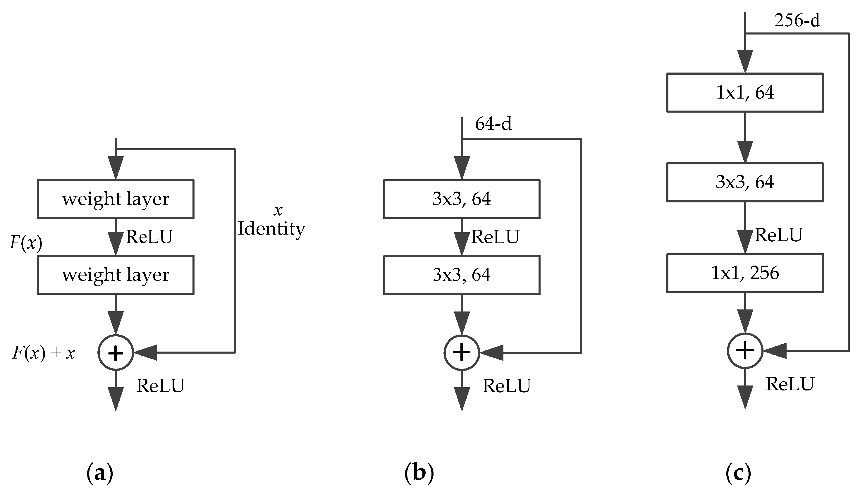
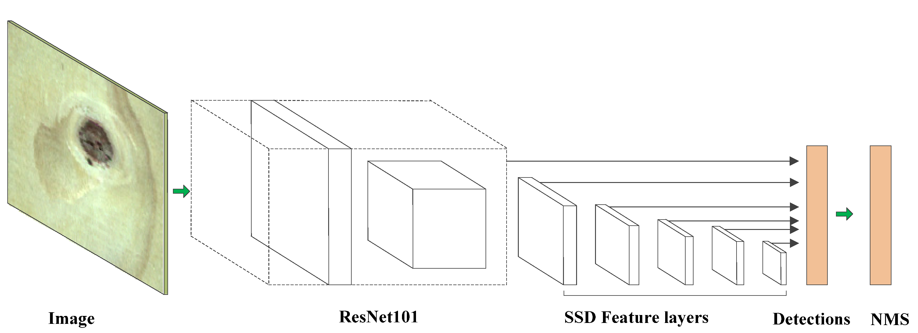
2.6. Deep Residual Network

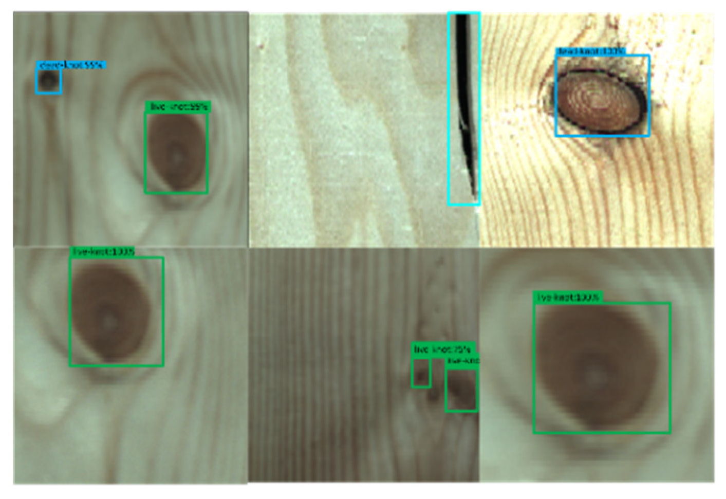
With the deepening of the network, there is a phenomenon that the accuracy of the training set decreases due to non-overfitting [29]. He [30] put forward a new kind of network structure for this problem, namely the Deep Residual Network, also known as ResNet. ResNet allows the network to be deepened as much as possible. The Shortcut Connection structure is introduced to transform the direct mapping of the original deep network into a residual mapping. When the parameter is passed, some layers will be skipped and directly enter the subsequent network layer, thereby reducing the complexity of the model.

The Shortcut Connection of ResNet is shown in Figure 6a. There are two types of mapping: Identity Mapping and Residual Mapping. Identity Mapping refers to the part $x$ that is directly connected by skipping two weight layers in the above figure, and the other Residual Mapping refers to the part $F\left(x\right)$ that passes through two weight layers, so the final output is $y=F\left(x\right)+x$. Generally, each Shortcut Connection structure is called a building block. If the network has reached the optimal level, continuing to deepen the network, Residual Mapping will be ignored and only Identity Mapping is left. In theory, the network is kept in an optimal state, and the performance of the network will gradually improve as the depth increases. Figure 6b,c are two designs of Shortcut Connection with similar time complexity. We chose ResNet101 (structure (b) shown in Figure 6), using the first 1 × 1 convolution to reduce the dimension of the current feature map to 64 dimensions, and finally restored it to the original dimension through 1 × 1 convolution. The number of parameters used totally is: 1 × 1 × 256 × 64 + 3 × 3 × 64 × 64 + 1 × 1 × 64 × 256 = 69,632, and without the Bottleneck structure, the parameters needed would be two convolutions of 3 × 3 × 256, and the number of parameters at this time would be: 3 × 3 × 256 × 256 × 2 = 1,179,648. By using ResNet, we reduce the calculation of parameters by nearly 17 times.

The application of a deep residual network can avoid the network degradation and precision decline caused by the increase in depth of the VGG network. It can also optimize the performance of the SSD algorithm and improve the detection speed and accuracy of the SSD model. After selecting the ResNet101 network to replace the VGG16 network, the original SSD network framework becomes the structure shown in Figure 7.

3. Results

First, we use the SSD network structure shown in Figure 5 to develop an SSD algorithm program based on the TensorFlow deep learning framework and input the newly collected 300 × 300 RGB solid wood board images into the SSD program. The number of training iterations is set to 20,000, the accuracy of the recognition is judged by the confidence of the predicted rectangular frame to obtain the position of the predicted rectangular frame (center coordinates, length and width) as the positioning information to identify the target, and the recognition results are shown in

Table 2. Detection results of the detection model.

Wood Defect	ResNet + SSD Algorithm		SSD Algorithm
	Accuracy of Training Set	Accuracy of Test Set	Accuracy of Training Set	Accuracy of Test Set
Live knot	0.984	0.970	0.962	0.917
Dead knot	0.962	0.924	0.936	0.884
Decay	0.922	0.875	0.884	0.804
Mildew	0.912	0.860	0.801	0.700
Crackle	0.992	0.967	0.995	0.956
Pinhole	0.838	0.786	0.625	0.455
Average accuracy	0.935	0.897	0.867	0.786
Average detection time	90 ms		116 ms

.

As shown in Table 2, the average recognition rate of the surface defects of a solid wood panel using the general SSD algorithm is 0.867. The detection accuracy is not enough, which cannot meet the requirements of industrial applications. Not only does it miss the detection, but it also deviates from the envelope of the target bounding box, especially the recognition rate of small targets, such as holes, is lower than 0.5, so the algorithm still needs to be improved. Therefore, the traditional SSD algorithm is optimized in this paper.

The ResNet network is used to replace the VGG network part on the basis of the SSD network. The improved network structure is shown in Figure 7. During training, the original SSD model parameters are used as the initialization parameters of the improved model for adjustment, and the maximum number of training iterations is set to 20,000. The recognition results are shown in Table 2. The ResNet + SSD model has good detection performance on defects such as live knots and dead knots compared with the traditional SSD model. For the same samples, the total recognition accuracy of the ResNet + SSD algorithm reached over 92%. Table 2 shows a comparison of the results of the two models.

In this paper, the ResNet + SSD algorithm is designed to detect the surface defects of the solid wood panel. The SSD algorithm involves the predicted box mechanism. After the solid wood panel image passes through the network, the specific recognition comparisons of the above-mentioned SSD algorithm and the improved algorithm are shown in Figure 8 and Figure 9. Figure 8 is the recognition result based on the SSD algorithm. Figure 9 is the recognition result based on the ResNet + SSD algorithm. Compared with Figure 8 and Figure 9, the ResNet + SSD algorithm can detect the defects that the SSD algorithm can detect while detecting smaller defects and obtaining higher accuracy.

4. Discussion and Conclusions

In order to improve the performance of the traditional image processing method to detect solid wood defects, this paper proposes an improved SSD solid wood defects detection model improved with ResNet to target and identify major defects such as knots, decay, mildew, crackle and pinhole. The detection results show that the performance of the proposed model meets the needs of industrial production. The average detection accuracy of surface defects detected by the SSD algorithm is 0.8666, and the average detection time is 116 ms. Although the SSD structure has good recognition performance on knots and cracks, it has poor recognition performance on small defects. Therefore, ResNet is used to replace the VGG-16 network in the original SSD algorithm. The original SSD model parameters are used as the initialization parameters of the improved model to adjust the network structure. This avoids network degradation while increasing the number of network layers to improve detection accuracy. By comparing and analyzing the SSD and the ResNet + SSD algorithms, it is concluded that the detection accuracy and detection time of the SSD algorithm optimized by ResNet are improved by 0.141 and 0.2241 compared to the SSD algorithm, respectively, which can more accurately and quickly identify and locate defects.

In this paper, the detection of the surface defects of solid wood panels only stays at the stage of single-sided detection, and the double-sided detection of solid wood panels needs to be realized in the future. At the same time, we optimized the SSD algorithm and improved the detection accuracy and detection time, but the envelope deviation of the target bounding box still exists. The algorithm should be further improved at a later time to improve the detection performance.

References

1. He, T.; Liu, Y.; Xu, C.Y.; Zhou, X.L.; Hu, Z.K.; Fan, J.N. A Fully Convolutional Neural Network for Wood Defect Location and Identification. IEEE Access 2019, 7, 123453–123462. [Google Scholar] [CrossRef]
2. He, T.; Liu, Y.; Yu, Y.B.; Zhao, Q.; Hu, Z.K. Application of deep convolutional neural network on feature extraction and detection of wood defects. Measurement 2020, 152, 107357. [Google Scholar] [CrossRef]
3. Shi, J.H.; Li, Z.Y.; Zhu, T.T.; Wang, D.Y.; Ni, C. Defect Detection of Industry Wood Veneer Based on NAS and Multi-Channel Mask R-CNN. Sensors 2020, 20, 4398. [Google Scholar] [CrossRef] [PubMed]
4. Sandak, J.; Orlowski, K.A.; Sandak, A.; Chuchala, D.; Taube, P. On-Line Measurement of Wood Surface Smoothness. Drv. Ind. Znan. Čas. Pitanja Drv. Tehnol. 2020, 71, 193–200. [Google Scholar] [CrossRef]
5. Tondon, A.; Singh, M.; Sandhu, B.S.; Singh, B. Importance of Voxel Size in Defect Localization Using Gamma-Ray Scattering. Nucl. Sci. Eng. 2019, 193, 1265–1275. [Google Scholar] [CrossRef]
6. Li, S.L.; Li, D.J.; Yuan, W.Q. Wood Defect Classification Based on Two-Dimensional Histogram Constituted by LBP and Local Binary Differential Excitation Pattern. IEEE Access 2019, 7, 145829–145842. [Google Scholar] [CrossRef]
7. Ji, X.; Guo, H.; Hu, M. Features Extraction and Classification of Wood Defect Based on Hu Invariant Moment and Wavelet Moment and BP Neural Network. In Proceedings of the 12th International Symposium on Visual Information Communication and Interaction, New York, NY, USA, 20–22 September 2019. [Google Scholar]
8. Bandara, S.; Rajeev, P.; Gad, E.; Sriskantharajah, B.; Flatley, I. Damage detection of in service timber poles using Hilbert-Huang transform. NDT E Int. 2019, 107, 15. [Google Scholar] [CrossRef]
9. Li, B.; Wu, Y.; Guo, F.X.; Qi, J. Real-Time Detection Method for Surface Defects of Stamping Parts Based on Template Matching. In Proceedings of the 2018 4th International Conference on Environmental Science and Material Application, Xi’an, China, 15–16 December 2018; Iop Publishing Ltd.: Bristol, UK, 2019; Volume 252. [Google Scholar]
10. Ruz, G.; Estevez, P.; Perez, C. A Neurofuzzy Color Image Segmentation Method for Wood Surface Defect Detection. For. Prod. J. 2005, 55, 52–58. [Google Scholar]
11. Li, C.; Zhang, Y.Z.; Tu, W.J.; Jun, C.; Liang, H.; Yu, H.L. Soft measurement of wood defects based on LDA feature fusion and compressed sensor images. J. For. Res. 2017, 28, 1285–1292. [Google Scholar] [CrossRef]
12. Gao, M.; Qi, D.; Mu, H.; Chen, J. A Transfer Residual Neural Network Based on ResNet-34 for Detection of Wood Knot Defects. Forests 2021, 12, 212. [Google Scholar] [CrossRef]
13. Tu, Y.X.; Ling, Z.G.; Guo, S.Y.; Wen, H. An Accurate and Real-Time Surface Defects Detection Method for Sawn Lumber. IEEE Trans. Instrum. Meas. 2021, 70, 11. [Google Scholar] [CrossRef]
14. Urbonas, A.; Raudonis, V.; Maskeliunas, R.; Damasevicius, R. Automated Identification of Wood Veneer Surface Defects Using Faster Region-Based Convolutional Neural Network with Data Augmentation and Transfer Learning. Appl. Sci. 2019, 9, 4898. [Google Scholar] [CrossRef] [Green Version]
15. Zhang, Y.Z.; Xu, C.; Li, C.; Yu, H.L.; Cao, J. Wood defect detection method with PCA feature fusion and compressed sensing. J. For. Res. 2015, 26, 745–751. [Google Scholar] [CrossRef]
16. Xie, Y.H.; Wang, J.C. Study on the identification of the wood surface defects based on texture features. Optik 2015, 126, 2231–2235. [Google Scholar]
17. Peng, Z.; Yue, L.; Xiao, N. Simultaneous Wood Defect and Species Detection with 3D Laser Scanning Scheme. Int. J. Opt. 2016, 2016, 7049523. [Google Scholar] [CrossRef]
18. Wang, C.; Liu, Y.; Wang, P.J.A. Extraction and Detection of Surface Defects in Particleboards by Tracking Moving Targets. Algorithms 2018, 12, 6. [Google Scholar] [CrossRef] [Green Version]
19. Pahlberg, T.; Thurley, M.; Popovic, D.; Hagman, O. Crack detection in oak flooring lamellae using ultrasound-excited thermography. Infrared Phys. Technol. 2018, 88, 57–69. [Google Scholar] [CrossRef] [Green Version]
20. Yang, J.; Zheng, X.; Yao, J.; Xiao, J.; Yan, L. 3D Surface Defects Recognition of Lumber and Straw-Based Panels Based on Structure Laser Sensor Scanning Technology. INMATEH-Agric. Eng. 2019, 57, 225–232. [Google Scholar]
21. Badrinarayanan, V.; Kendall, A.; Cipolla, R. SegNet: A Deep Convolutional Encoder-Decoder Architecture for Image Segmentation. IEEE Trans. Pattern Anal. Mach. Intell. 2017, 39, 2481–2495. [Google Scholar] [CrossRef]
22. Guo, X.P.; Nie, R.C.; Cao, J.D.; Zhou, D.M.; Qian, W.H. Fully Convolutional Network-Based Multifocus Image Fusion. Neural Comput. 2018, 30, 1775–1800. [Google Scholar] [CrossRef]
23. Nian, R.; He, B.; Lendasse, A. 3D object recognition based on a geometrical topology model and extreme learning machine. Neural Comput. Appl. 2013, 22, 427–433. [Google Scholar] [CrossRef]
24. Huang, G.B.J.C.C. What are Extreme Learning Machines? Filling the Gap between Frank Rosenblatt’s Dream and John von Neumann’s Puzzle. Cogn. Comput. 2015, 7, 263–278. [Google Scholar] [CrossRef]
25. Chau, V.H.; Vo, A.T.; Le, B.T. A Gravitational-Double Layer Extreme Learning Machine and Its Application in Powerlifting Analysis. IEEE Access 2019, 7, 143990–143998. [Google Scholar] [CrossRef]
26. Liu, W.; Anguelov, D.; Erhan, D.; Szegedy, C.; Reed, S.; Fu, C.Y.; Berg, A.C.J.S. SSD: Single Shot MultiBox Detector. In Proceedings of the Computer Vision—ECCV 2016, 14th European Conference, Amsterdam, The Netherlands, 11–14 October 2016; Springer: Cham, Switzerland, 2016. [Google Scholar]
27. Simonyan, K.; Zisserman, A.J.C.S. Very Deep Convolutional Networks for Large-Scale Image Recognition. arXiv 2014, arXiv:1409.1556. [Google Scholar]
28. Girshick, R.; Donahue, J.; Darrell, T.; Malik, J. Rich feature hierarchies for accurate object detection and semantic segmentation. In Proceedings of the IEEE Conference on Computer Vision and Pattern Recognition, Columbus, OH, USA, 23–28 June 2014; pp. 580–587. [Google Scholar]
29. Jia, S.; Deng, L.; Shen, L.L. An Effective Collaborative Representation Algorithm for Hyperspectral Image Classification. In Proceedings of the 2014 IEEE International Conference on Multimedia and Expo (ICME), Chengdu, China, 14–18 July 2014. [Google Scholar]
30. He, K.M.; Zhang, X.Y.; Ren, S.Q.; Sun, J. Identity Mappings in Deep Residual Networks. In Proceedings of the Computer Vision—ECCV 2016, 14th European Conference, Amsterdam, The Netherlands, 11–14 October 2016; Springer: Cham, Switzerland, 2016; Volume 9908, pp. 630–645. [Google Scholar]
Figure 1. Image acquisition device for solid wood surface defects.
Forests 12 01419 g001
Figure 2. Partial sample images.
Forests 12 01419 g002
Figure 3. Image data enhancement. (a) Mirrored or rotated images at different angles. (b) Changed image contrast. (c) Scaled image at a scale of 0.8 and 1.2.
Forests 12 01419 g003
Figure 4. Partially annotated sample images. Different colored boxes indicate different defects, green colored boxes indicate live knots, blue colored boxes indicate dead knots, and red colored boxes indicate mildew, etc.
Forests 12 01419 g004
Figure 5. General framework of the SSD algorithm.
Forests 12 01419 g005
Figure 6. Design of shortcut connection structures of ResNet. (a) A building block. (b) ResNet34. (c) ResNet50/101/152.
Forests 12 01419 g006
Figure 7. Improved SSD network framework based on the ResNet network.
Forests 12 01419 g007
Figure 8. Recognition results based on the SSD algorithm.
Forests 12 01419 g008
Figure 9. Recognition results based on the ResNet + SSD algorithm.
Forests 12 01419 g009