The Temporal Variation of the Microclimate and Human Thermal Comfort in Urban Wetland Parks: A Case Study of Xixi National Wetland Park, China

Abstract

As an important part of the ecological infrastructure in urban areas, urban wetland parks have the significant ecological function of relieving the discomfort of people during their outdoor activities. In recent years, the specific structures and ecosystem services of urban wetland parks have been investigated from different perspectives. However, the microclimate and human thermal comfort (HTC) of urban wetland parks have rarely been discussed. In particular, the changing trends of HTC in different seasons and times have not been effectively presented. Accordingly, in this research, a monitoring platform was established in Xixi National Wetland Park, China, to continually monitor its microclimate in the long term. Via a comparison with a control site in the downtown area of Hangzhou, China, the temporal variations of the microclimate and HTC in the urban wetland park are quantified, and suggestions for clothing are also provided. The results of this study demonstrate that urban wetland parks can mitigate the heat island effect and dry island effect in summer. In addition, urban wetland parks can provide ecological services at midday during winter to mitigate the cold island effect. More importantly, urban wetland parks are found to exhibit their best performance in improving HTC during the daytime of the hot season and the midday period of the cold season. Finally, the findings of this study suggest that citizens should take protective measures and enjoy their activities in the morning, evening, or at night, not at midday in hot weather. Moreover, extra layers are suggested to be worn before going to urban wetland parks at night in cold weather, and recreational activities involving accommodation are not recommended. These findings provide not only basic scientific data for the assessment of the management and ecological health value of Xixi National Wetland Park and other urban wetland parks with subtropical monsoon climates, but also a reference for visitor timing and clothing suggestions for recreational activities.

1. Introduction

Due to the complex social process of rapid urbanization, approximately half of the global population lives in urban areas, and this percentage is still increasing [1,2]. Undeniably, modernized fundamental infrastructure has provided great convenience to human life. Compared to a century ago, people living in urban areas work efficiently and create high economic value. However, due to rapid urbanization, factors such as the expansion of urban areas, the use of concrete and asphalt, and the loss of natural resources and space have led to increased and decreased temperatures in urban areas in summer and winter, respectively, as well as reduced humidity, compared to rural areas. These phenomena are respectively known as the urban heat (cold) island effect and the urban dry island effect [2]. Furthermore, in the context of global climate change, extreme weather events, including urban waterlogging, dry winds, and persistent heat and cold waves, are frequently observed in urban areas [3,4]. This can be attributed to the spatial heterogeneity and fragmentation of the urban environment. Human-induced urban spaces cause damage to the essential functions of natural ecosystems, including substance circulation, energy exchange, and information transfer. Indeed, urban ecosystems cannot regulate their temperature independently, as the concrete ground is directly exposed to sunlight, and air conditioners and other electrical devices are widely used [5]. This results in the incapability of the urban ecosystem to effectively exert its ecological function of adjusting the microclimate, leading to the growing discomfort of people during their outdoor activities [6].

The ecological infrastructure plays an important role in maintaining the integrity of the urban ecological structure. Due to the COVID-19 pandemic, people are required to maintain social distance. In this case, there has been more awareness of the significance of natural outdoor space and fresh air. As one of the most important ecological infrastructures in urban areas, wetland parks provide various ecosystem services, including climate regulation, flood control, aquifer recharging, water purification, carbon sequestration, and they act as habitats for plants and animals [7,8,9]. In recent years, the specific structures and ecosystem services of wetland parks have been investigated from different perspectives [10,11,12]. The human thermal comfort (HTC) of the environment is also an important component of ecosystem services and plays a vital role in improving the physical and mental health of visitors in wetland parks. Unfortunately, the HTC of urban wetland parks has rarely been discussed.

HTC, which is a concept that reflects humans’ perception of the thermal environment, has been widely employed to evaluate the comfort level of the body in response to the environment [13,14]. The traditional method of the measurement of HTC is to use a series of meteorological factors (e.g., temperature, humidity, wind speed, radiation, etc.) to establish a comprehensive index by which to quantify the bioclimatic conditions for human. Over the past century, more than 100 indices have been developed and used to assess HTC in combination with meteorological factors [15]. In recent years, several models, such as the urban canopy model, Urban Tethys-Chloris (UT&C), have been proposed to evaluate the urban thermal climate. UT&C is a combination of an urban canyon scheme and an ecohydrological model, and considers air and surface temperatures, air humidity, and soil moisture, as well as the urban energy and hydrological fluxes in the absence of snow [16,17,18]. These indexes and models all provide the basis for assessing the human thermal sensation of the environment. Previous studies of microclimates and HTC focused on urban outdoor spaces, college campuses, street green spaces, and city parks [19,20,21,22,23]. However, most of these studies were conducted in the summer, and the monitoring periods tended to be short (typically 3–7 d). Additionally, some studies did not consider the effects of relative humidity and wind speed on HTC, and continual monitoring in the long term was not sufficient, leading to the ineffective presentation of the changing trends of HTC in different seasons and at different times.

Therefore, based on the annual monitoring of the microclimate features and HTC of Xixi National Wetland Park, China in different seasons, this study determines the period of time in a day when people can obtain the highest level of HTC during recreational activities, and offers suggestions for appropriate clothing. The results provide a reference for the design and management of ecology therapy activities in wetland parks.

2. Target Site and Methods

2.1. Target Site

In this study, Xixi National Wetland Park in China was selected as the target site. Xixi National Wetland Park (30°15.39′ N–30°16.96′ N, 120°03.16′ E–120°04.94′ E) is 16 km from the downtown area of Hangzhou, China. As a typical urban wetland park and China’s first national wetland park, Xixi National Wetland Park was established by the State Forestry and Grassland Administration (formerly the State Forestry Administration) of China in 2005 [24]. It has a total area of 11.5 km², and over 50% of its surface is covered by water. The park has a typical humid subtropical monsoon climate with high temperatures and precipitation in summer, and low precipitation in winter. The average temperature is about 16.2 °C, and the average precipitation is about 1400 mm per year. Xixi National Wetland Park consists of three areas: the wetland ecological protection and cultivation area (east), the wetland eco-tourism leisure area (center), and the wetland ecological landscape conservation area (west). As shown in Figure 1, the wetland park site (WPS) and the control site (CS) are in the ecological protection and cultivation area and the downtown area of Hangzhou, respectively. When the positioning monitoring platform used in this study was installed, the destruction of vegetation around the site was minimized. After installation, the original vegetation was reconstructed. Excluding the presence of protective measures, such as a guardrail installed around the site, there is no man-made shade or open space to prevent the modification of wind flow and the limiting of heat dissipation. The CS is not shaded by nearby buildings, and is not affected by wind channelling, downdraft effects, etc. Thus, the microclimate characteristics of the regions represented by the two platforms are objectively reflected.

2.2. Methods

2.2.1. Monitoring and Data Sources

At each site, a monitoring platform was set up to monitor the air temperature, relative humidity, and wind speed, as shown in Figure 1. The air temperature and relative humidity were detected by a sensor (Vaisala HMP155, Vaisala, Inc., Woburn, USA), and the wind speed was measured by an anemometer (RM Young Wind Sentry Set03002-1, Campbell Scientific Inc., Logan, USA) 24 h per day.

The data collector (CR1000, Campbell Scientific Inc., Logan, USA) recorded data every 15 min and transmitted it to a remotely controlled computer via the MA8-L GPRS terminal. The description of measuring devices is provided in

Table 1. The description of measuring sensors.

Sensors	Product Type	Work Environment	Measuring Range	Accuracy
Temperature and humidity sensor	HMP155		−40–60 °C, 0–60 %	±0.2 °C, ±1%
Anemometer	Set03002-1	−20–50 °C	0–60 m/s	±0.5 m/s
Data collector	CR1000	−20–65 °C

. In this study, data collected from January–December 2016 were used.

2.2.2. Assessment Indicators of HTC

Table 1 reports the common indices of HTC used internationally, each of which has its own applicable weather conditions. By comparing various indices, Blazejczyk et al. confirmed that each index has a high correlation with each other (the lowest R² coefficient was 93.1), regardless of the inclusion of a radiation factor in the equation. Moreover, it was pointed out that non-radiation equations are used more widely in some climatic conditions [15]. In other words, each index demonstrates high consistency in the assessment of HTC. Therefore, in the application of bioclimatic indices for the assessment of HTC, the climatic conditions of the research area and people’s thermal perception habits should be fully considered during index selection.

Similar to the indices listed in

Table 2. The combined environmental variables and applicable weather conditions of indices.

Indices	Combined Environmental Variables	Applicable Weather Conditions	References
Heat index (HI)	Air temperature and relative humidity	Hot weather	Steadman [25]
Humidex (HD)	Air temperature and air vapor pressure	Hot weather	Sirangelo et al. [26] and Masterton and Richardson [27]
Effective temperature (ET)	Air temperature, relative humidity, and wind speed	Hot and warm weather	Houghton and Yaglou [28]
Wet-bulb globe temperature (WBGT)	Air temperature, globe temperature, and natural wet bulb temperature	Hot weather	ISO 7243 [29] and d’Ambrosio Alfano et al. [30]
Wind chill index (WCI)	Air temperature and wind speed	Cold weather	Lin et al. [31] and Blazejczyk et al. [15]
Standard effective temperature (SET)	Air temperature, relative humidity, and mean radiant temperature	Hot weather	Gagge et al. [32] and Gagge et al. [33]
Insulation required (IREQ)	Air temperature, mean radiant temperature, relative humidity, and air velocity	Cold weather	ISO 11079 [34] and d’Ambrosio Alfano et al. [35]
Predicted heat strain (PHS)	Air temperature, mean radiant temperature, relative humidity, and air velocity	Hot weather	ISO 7933 [36] and d’Ambrosio Alfano et al. [37]
Physiological equivalent temperature (PET)	Air temperature, air vapor pressure, wind speed, and mean radiant temperature	Hot and cold weather	Höppe [38]
Universal Thermal Climate Index (UTCI)	Air temperature, mean radiant temperature, air vapor pressure, and wind speed	Hot and cold weather	Jendritzky et al. [39]

, the indices reported in

Table 3. The most widely used indices in China.

Indices	Combined Environmental Variables	Equations *	Applicable Weather Conditions
Human thermal comfort index (HTCI)	Air temperature, relative humidity, and wind speed	HTCI = $0.6\times \left(\left|T-24\right|\right)+0.07\times \left(\left|RH-70\right|\right)+0.5\times \left(\left|V-2\right|\right)$	Hot and cold weather
Thermal humidity index (THI)	Air temperature and relative humidity	THI = $T-0.55\times \left(1-RH\right)\left(T-14.5\right)$	Hot weather
Human comfort index (HCI)	Air temperature, relative humidity, and wind speed	HCI = $1.8T-0.55\times \left(1.8T-26\right)\left(1-RH\right)-3.2\times \sqrt{V}+32$	Hot and cold weather
Discomfort index (DI)	Air temperature and relative humidity	DI = $1.8T+32-0.55\times \left(1-RH\right)\left(1.8T-26\right)$	Hot weather
Cool index (CI)	Air temperature, and wind speed	CI = $\left(10\times \sqrt{V}+10.45-V\right)\left(33-T\right)$	Cold weather

* T is the temperature (°C), RH is the relative humidity (%), and V is the wind speed (m/s).

are the most widely used in China. In comprehensive consideration of the scope of application of each index and the seasonal dressing habits of the Chinese people, the human thermal comfort index (HTCI) and clothing thickness index (CTI) were employed to evaluate the human perception of the environment. The HTCI was focused on evaluating the comfort level of the body. Additionally, the CTI can serve as an indicator of clothing.

(1) The HTCI, proposed by Lu et al. [40], is a synthesis of temperature, relative humidity, and wind speed, and is calculated by the following Equation (1) [41,42]. Compared to the thermal humidity index (which is only applicable to hot climate conditions), the HTCI can better reflect the outdoor satisfaction level of humans in the four seasons, and thus it is widely applied.

$$\mathrm{HTCI}=0.6\times \left(\left|T-24\right|\right)+0.07\times \left(\left|RH-70\right|\right)+0.5\times \left(\left|V-2\right|\right),$$

(1)

where T is the temperature (°C), RH is the relative humidity (%), and V is the wind speed (m/s). The HTCI is negatively related to the body perception of comfort, as presented in

Table 4. The relationship between the HTCI and human body perception [41,42].

Level	Range	Feeling
I	HTCI ≤ 4.55	Very comfortable
II	4.55 < HTCI ≤ 6.95	Comfortable
III	6.95 < HTCI ≤ 9.00	Uncomfortable
IV	HTCI > 9.00	Very uncomfortable

.

(2) The CTI is also a synthesis of temperature, relative humidity, and wind speed, and is calculated by the following equations [41,43].

If T ≤ 18 °C and RH ≥ 60%,

$$\mathrm{CTI}=\frac{\left[1+\frac{0.4\left(RH-60\right)}{100}\right]\times 0.61\left(33-T\right)}{\left(1-0.01165V^2\right)}.$$

(2)

If 18 °C < T < 26 °C or T ≤ 18 °C, and RH < 60%, or, if T ≥ 26 °C and RH < 60%,

$$\mathrm{CTI}=\frac{0.61\left(33-T\right)}{\left(1-0.01165V^2\right)}.$$

(3)

If T ≥ 26 °C and RH ≥ 60%,

$$\mathrm{CTI}=\frac{\left[1-\frac{0.4\left(RH-60\right)}{100}\right]\times 0.61\left(33-T\right)}{\left(1-0.01165V^2\right)}.$$

(4)

In these equations, T is the temperature (°C), RH is the relative humidity (%), and V is the wind speed (m/s).

Table 5. Division of the CTI and clothing suggestion.

Level	Range	Clothing Suggestion
I	CTI ≤ 1.5	Short-sleeve-based summer clothing
II	1.5 < CTI ≤ 6	Long-sleeve shirt
III	6 < CTI ≤ 11	Shirts plus a jacket or suit
IV	11 < CTI ≤ 18	Sweater plus a thin coat or thin cotton coat
V	CTI > 18	Thick sweater plus a wool coat or down jacket or other winter clothing

presents the relationship between the CTI and the clothing suggestion, which was adapted from the work of Gu et al. [41] and Zhu et al. [43].

2.2.3. Data Analysis

Herein, spring refers to the months of March, April, and May, summer includes June, July, and August, autumn includes September, October, and November, and winter includes December, January, and February. The winter data considered in this study were collected in December, January, and February 2016.

When the observation data were obtained from the data collector, a quality check was carried out first. After removing the abnormal data, statistical analysis was performed. The temperature, relative humidity, and wind speed at the same time each day of the year were averaged to obtain microclimatic data at that time, from which the daily variations are plotted. After that, the temperature, relative humidity and wind speed in each month and season were averaged arithmetically, i.e., the microclimatic data of the month and season were obtained respectively. Finally, the daily, monthly, and seasonal variations of HTCI and CTI were calculated according to Equations (1)–(4). The significance of arithmetic mean values for all data sets was assessed using Student’s t-test. Error bars were calculated with the s.d. function. The differences at p < 0.05 were considered statistically significant by One-way ANOVA. According to the Student’s t-test, characters in the figure represent statistically significant differences compared with control (* p < 0.05, ** p < 0.01 and *** p < 0.001). Data analysis was conducted using SPSS 19.0 software (IBM^® SPSS^® software, Armonk, NY, USA), and the data were plotted by GraphPad Prism 8 software (GraphPad Software, Inc., San Diego, CA, USA).

3. Results

3.1. Seasonal, Monthly, and Daily Variations of the Microclimate

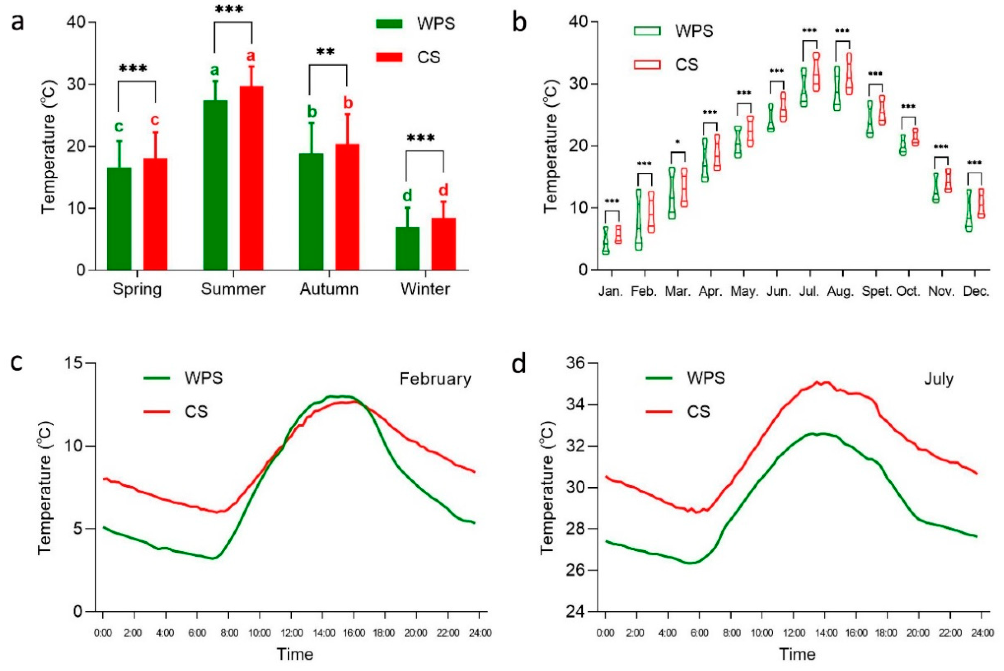
3.1.1. Seasonal, Monthly, and Daily Variations of Temperature

The seasonal variations of average temperature in both the WPS and CS exhibited a greater range in summer (27.5 and 29.7 °C) than in autumn (18.9 and 20.4 °C), spring (16.6 and 18.1 °C), and winter (7.0 and 8.5 °C) (Figure 2a). The monthly variation of the average temperature could be described as a unimodal curve, and in July and August, the peak values were reached in both the WPS and CS (Figure 2b). Regarding the daily variation, the average temperature exhibited a trend from decreasing to increasing, reached the highest point between 12:00 and 16:00, and then gradually decreased (Figure 2c,d and Supplementary Figure S1a–j). The seasonal, monthly, and daily variations of the temperature followed the natural laws of cool temperatures in the winter, warm temperatures in the summer, high temperatures during the day, and low temperatures at night. Moreover, the average temperature of the WPS in each season and month was significantly lower than that of the CS, and the percentage of reduction was between 6.30% and 20.83%. However, in terms of the daily variation, some interesting findings were discovered. Taking February as an example (Figure 2c), the average temperature of the WPS was higher than that of the CS between 11:45 and 16:30. This also occurred in March, January, and December (Supplementary Figure S1a,b,j). In other months, the average temperature of the WPS was lower than that of the CS in the 24-h cycle (Supplementary Figure S1c–i). Compared to the urban environment, the ecological infrastructures in the wetland park can reform the wind pattern and limit heat dissipation at noon in the cold season, so that more heat can be stored in the environment. Figure 2d presents the daily variation of temperature in July.

3.1.2. Seasonal, Monthly, and Daily Variations of Relative Humidity

The average relative humidity in both the WPS and CS differed with various seasons. It peaked in autumn (85.45% and 75.03%), followed by summer (83.34% and 68.74%) and spring (79.30% and 67.97%), and the lowest average relative humidity occurred in winter (77.08% and 65.32%). The average relative humidity of the WPS presented significant differences between the four seasons, while that of the CS exhibited no significant difference between spring and summer and had a significant difference with other seasons (Figure 3a). Regarding the monthly variation, the relative humidity was at a relatively high level in all months, there were negligible changes excluding February and August (Figure 3b). The daily variation of the average relative humidity first increased and then decreased, reached the lowest point at 14:40–16:00, and then increased gradually. In February, the average relative humidity of the WPS and CS was relatively close, between 11:45 and 16:30, while the percentage increase of relative humidity in the WPS was less than 10% that in the CS (Figure 3c). This was also observed in January, March, and December (Supplementary Figure S2a,b,j). In other months, the percentage increase of relative humidity was generally above 10% most of the day and overnight (Supplementary Figure S1c–i). Figure 3d presents the daily variation of the relative humidity in August. The average relative humidity of the WPS and CS exhibited significant differences on monthly and annual scales. Moreover, the average relative humidity of the WPS in each season and month was significantly higher than that of the CS, and the percentage increase was between 12.77% and 24.77%.

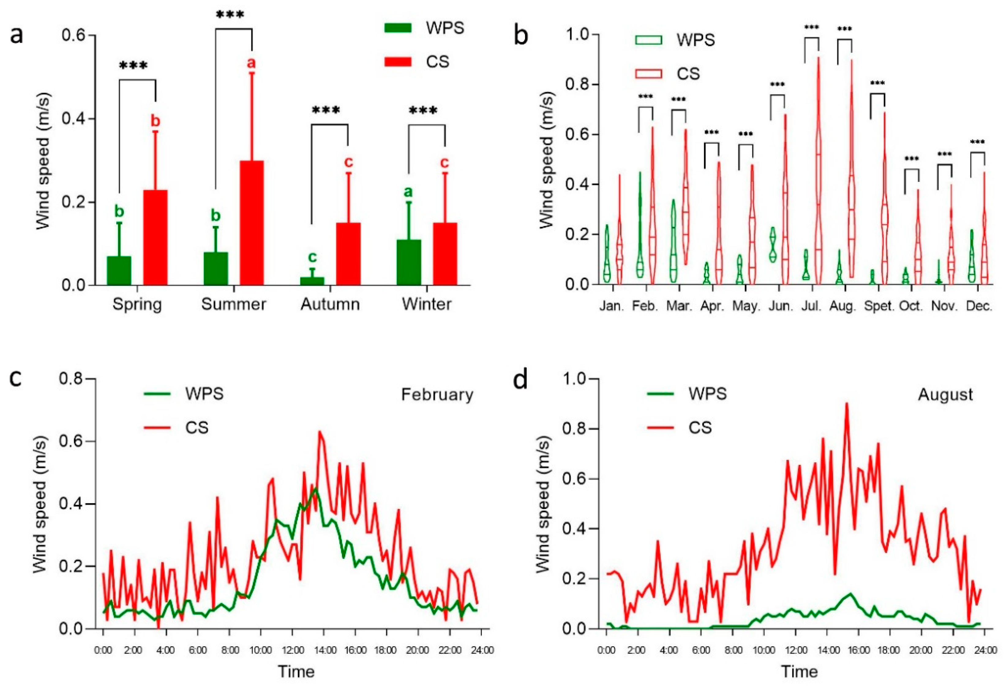
3.1.3. Seasonal, Monthly, and Daily Variations of Wind Speed

The wind speed in both the WPS and CS exhibited seasonal variation, and the wind speed in the WPS was significantly lower than that in the CS. The highest wind speed in the WPS occurred in winter (0.11 m/s), followed by summer (0.08 m/s) and spring (0.07 m/s), and the lowest wind speed occurred in autumn (0.02 m/s). The wind speeds in spring and summer were not substantially different, but recorded a large difference compared with winter and autumn (p < 0.05). The highest wind speed in the CS occurred in summer (0.21 m/s), followed by spring (0.14 m/s), and the lowest wind speed occurred in winter and autumn (0.12 m/s), which demonstrated a significant variation as compared with spring and summer (p < 0.05) (Figure 4a).

The monthly wind speed in the WPS and CS displayed fluctuations. In general, the wind speed in the WPS was relatively high in December, January, February, March, and June, while that in the CS was relatively high in February, March, June, July, and August, and the dispersion of the wind speed value in the CS was relatively large (Figure 4b). The daily variation curve for each month reveals that the wind speed in both the WPS and CS was the highest between 14:00 and 16:00 with a single peak. The daily variation of the wind speed in the CS was large in each month, whereas that in the WPS exhibited small fluctuations between April and November (Supplementary Figure S3c–i) and large fluctuations in other months (Supplementary Figure S3a,b,j). Figure 4c,d presents the daily variation of wind speed in February and August.

3.2. Seasonal, Monthly, and Daily Variations of the HTCI

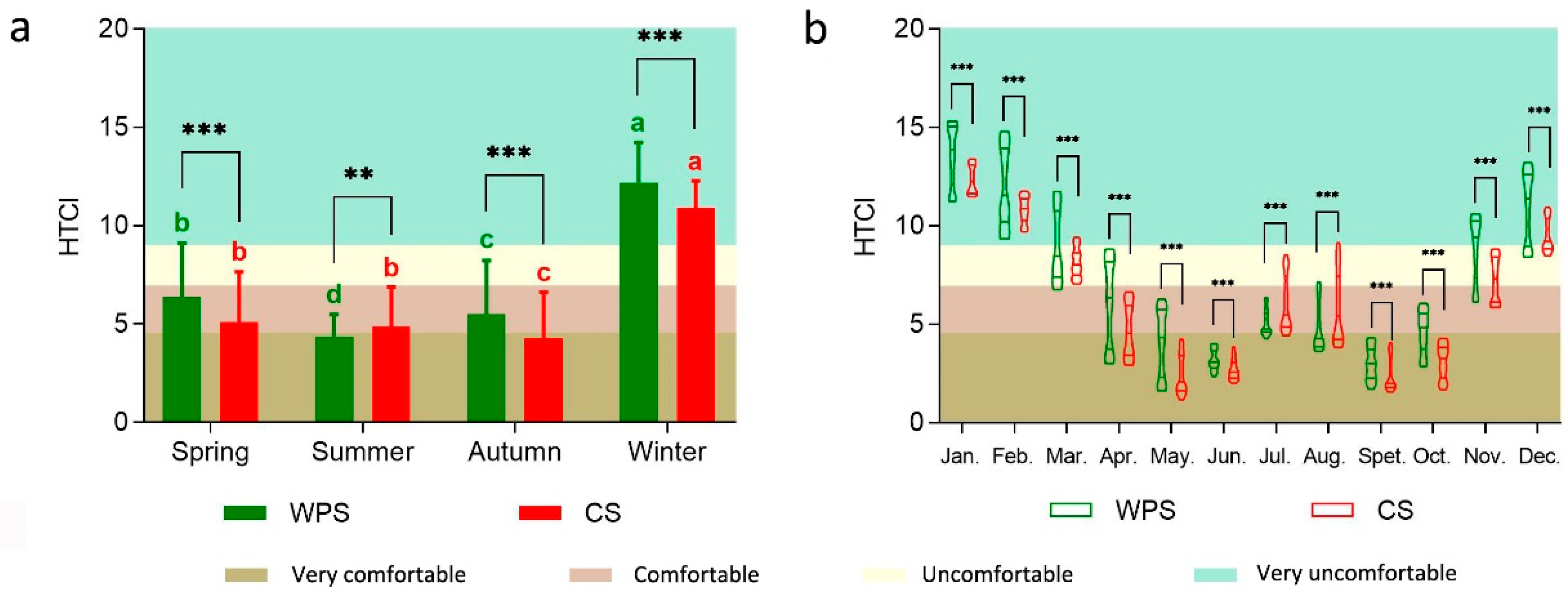
3.2.1. Seasonal and Monthly Variations of the HTCI and Human Body Perception

As shown in Figure 5a, the HTCI in both the WPS and CS demonstrated certain seasonal variations. Apart from summer, when the HTCI in the WPS was significantly lower than that in the CS (p < 0.01), the HTCI in the WPS was higher than that in the CS in the other seasons (p < 0.001). From the seasonal perspective, significant variations of the HTCI in the WPS between all seasons was observed (p < 0.05). The largest variation occurred in winter (12.17), which could be classified as a very uncomfortable feeling. The lowest variation occurred in summer (4.34), which could be classified as a very comfortable feeling. The variations in spring (6.38) and autumn (5.49) had a middle rank, which could be classified as a comfortable feeling. In the CS, the largest variation occurred in winter (10.90), which could be classified as a very uncomfortable feeling, the lowest variation occurred in autumn (4.26), which could be classified as a very comfortable feeling, and the variations in spring (5.09) and summer (4.86) had a middle rank, which could be classified as a comfortable feeling. The difference between spring and summer was not substantial, but their difference with winter and autumn was significant (p < 0.05).

The monthly HTCI in the WPS and CS exhibited a “W”-shaped trend. The value gradually decreased from January to May, slowly increased from June to July, decreased again from August to September, and then eventually increased. Apart from July and August, when the HTCI in the WPS was significantly lower than that in the CS (p < 0.001), the HTCI values in the WPS in all other months were larger than those in the CS. The WPS would have given people a very uncomfortable feeling in December, January, and February, an uncomfortable feeling in March and November, a comfortable feeling in April, July, August, and October, and a very comfortable feeling in May, June, and September (Figure 5b).

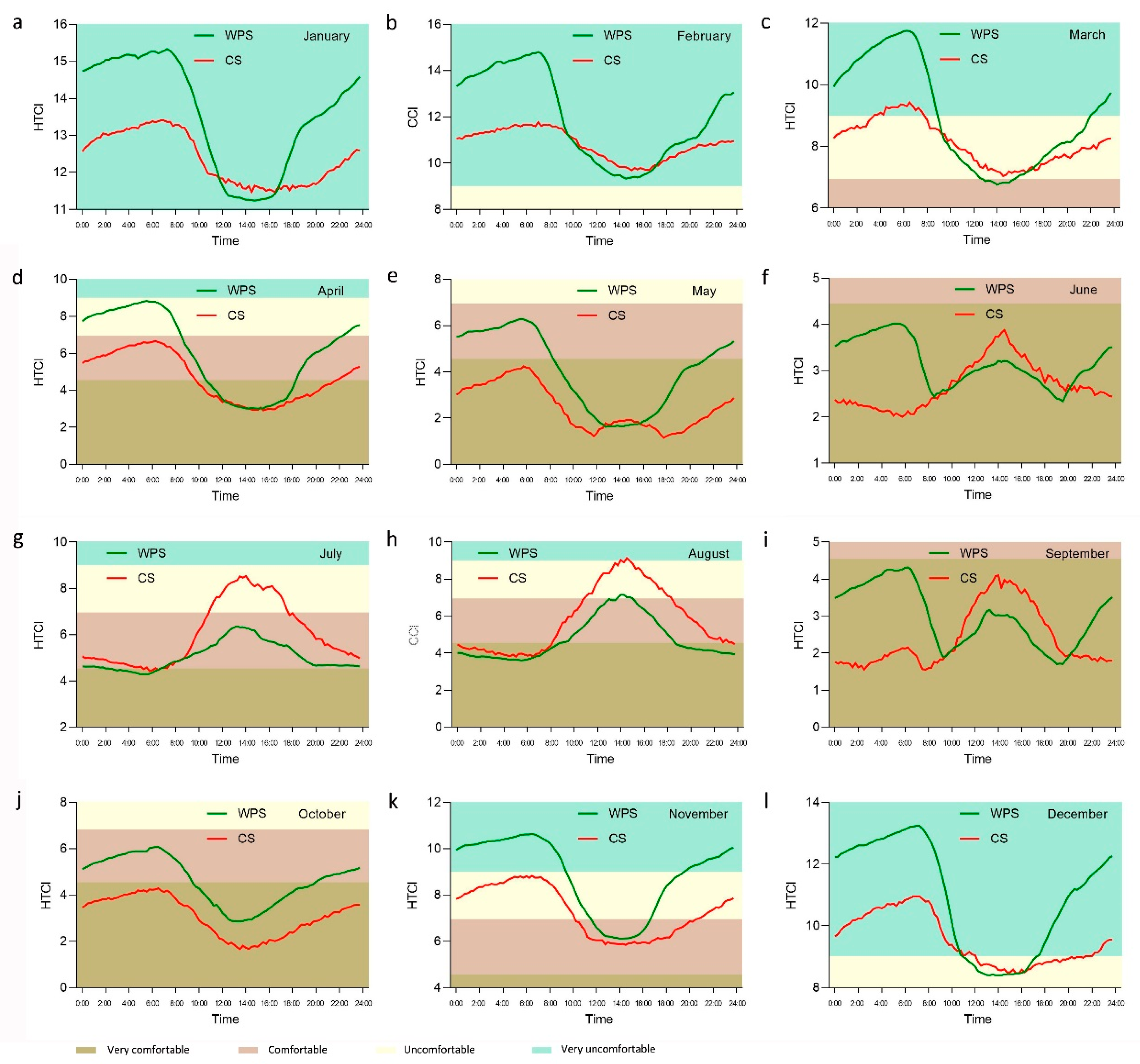
3.2.2. Daily Variation of the HTCI

As shown in Figure 6, the HTCI displayed different trends of daily variation over the 12-month observation period.

In January, February, March, April, October, November, and December, the HTCI in both the WPS and CS exhibited an increasing trend, then a decreasing trend, and finally rebounded. Two relationships existed between the WPS and CS in terms of the magnitude of the HTCI. Take February as an example. The HTCI in the WPS was lower than that in the CS during the period of 9:45–17:00, while it was higher than that in the CS in other periods (Figure 6b). The same relationship occurred in January, March, April, and December. In contrast, in October and November, the daily HTCI values in the WPS were higher than those in the CS in all time periods.

In May, the HTCI in the WPS exhibited a trend of increasing, decreasing, then increasing again, whereas the HTCI in the CS exhibited a “W”-shaped trend. During 12:45–15:30, the HTCI in the WPS was lower than that in the CS, whereas it was higher than that in the CS in other periods (Figure 6e).

In June and September, the HTCI in the WPS exhibited a “W”-shaped trend, while the HTCI in the CS presented a trend of decreasing followed by increasing and reached its peak at around 14:00, after which it slowly decreased (Figure 6f,i). The HTCI in the WPS was lower than that in the CS during the daytime. For example, in June, the HTCI in the WPS was lower than that in the CS during 9:45–20:00, but was higher than that in the CS in other periods (Figure 6f).

In July and August, the HTCI in both the WPS and CS exhibited a trend of increasing then decreasing, and reached its peak at around 14:00, whereas the HTCI in the WPS was lower than that in the CS in almost all time periods (Figure 6g,h).

3.2.3. Daily Variation of the Human Body Perception

As shown in Figure 6, in January, February, and December, the WPS and CS generated very uncomfortable or uncomfortable feelings all day long (Figure 6a,b,l). In March, the CS generated a very uncomfortable or uncomfortable feeling all day long, while the WPS generated a comfortable feeling during 12:45–15:30 but a very uncomfortable or uncomfortable feeling in other periods (Figure 6c). In April, the WPS generated a comfortable or very comfortable feeling during 8:30–22:15, but an uncomfortable feeling in other periods, while the CS generated a comfortable or very comfortable feeling all day long (Figure 6d). In July, the WPS generated a comfortable or very comfortable feeling all day long, while the CS generated an uncomfortable feeling during 11:00–17:30 but a comfortable or very comfortable feeling in other periods (Figure 6g). In August, the WPS generated an uncomfortable feeling during 13:45–15:00, but a comfortable or very comfortable feeling in other periods, while the CS generated a very uncomfortable or uncomfortable feeling during 11:00–18:15, but a comfortable or very comfortable feeling in other periods (Figure 6h). In November, the WPS generated a comfortable feeling during 11:45–16:30, but a very uncomfortable or uncomfortable feeling in other periods, while the CS generated a comfortable feeling during 10:15–20:30, but an uncomfortable feeling in other periods (Figure 6k). In May, June, September, and October, the WPS and CS both generated a comfortable or very comfortable feeling all day long (Figure 6e,f,i,j).

3.3. Seasonal, Monthly, and Daily Variations of the CTI

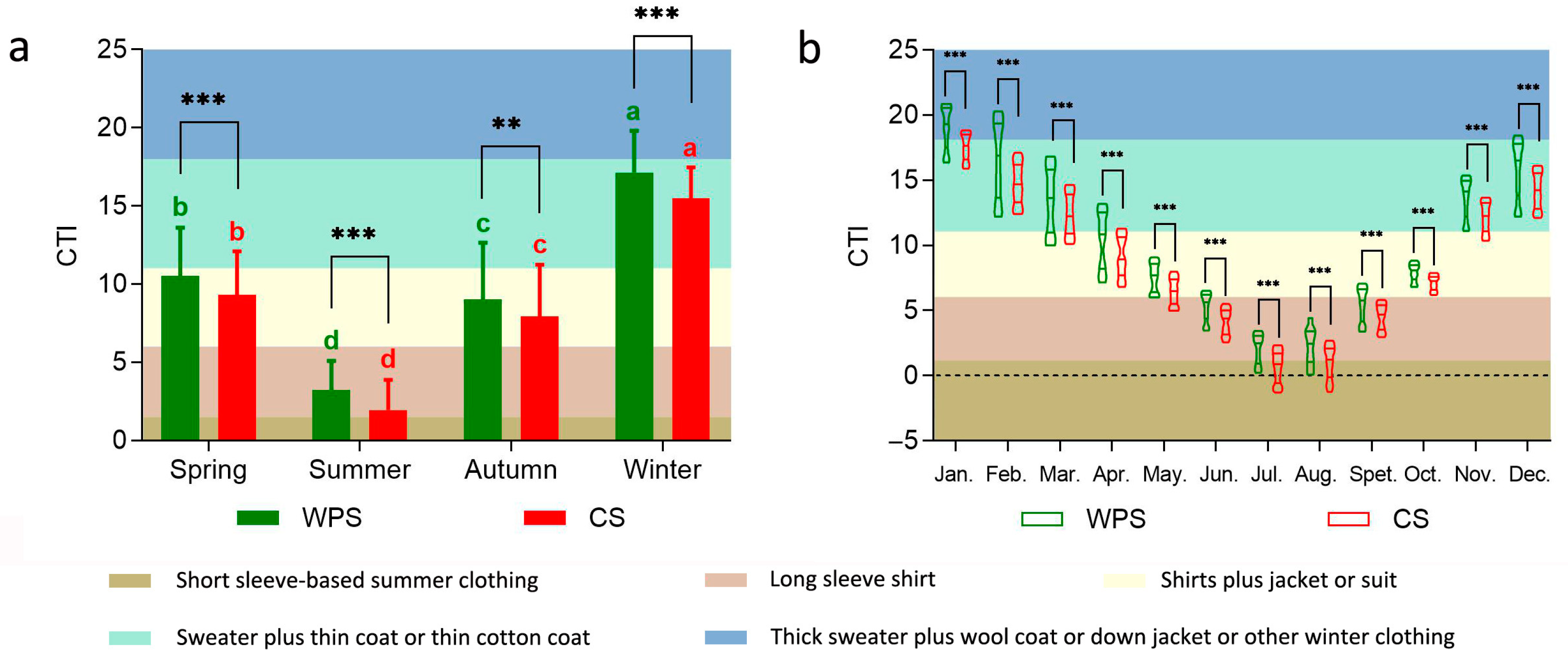
3.3.1. Seasonal and Monthly Variations of the CTI and Clothing Suggestions

As shown in Figure 7a, the CTI values in the WPS were all higher than those in the CS in all four seasons (p < 0.01). The CTI in the WPS and CS exhibited significant seasonal variations (p < 0.05), with winter displaying the highest values (17.14 and 15.49). This belongs to level IV, so a sweater in addition to a thin coat or thin cotton coat is recommended for outdoor activities. Summer had the lowest variations (3.21 and 1.94). This belongs to level II, so a long-sleeve shirt is recommended for outdoor activities. Spring (10.50 and 9.32) and autumn (9.03 and 7.93) ranked in the middle. These belong to level III, so a shirt in addition to a jacket or suit is recommended for outdoor activities.

From the monthly perspective, the CTI in the WPS and CS demonstrated a decreasing and then increasing trend, with July having the lowest variation (−2.06 and 0.68). The CTI values in the WPS were all higher than those in the CS in each month (p < 0.01). In January, the CTI in the WPS belonged to level V, so a thick sweater in addition to a wool coat or down jacket or other winter clothing is recommended for outdoor activities. In the CS, the CTI belonged to level IV, so a sweater in addition to a thin coat or thin cotton coat is recommended for outdoor activities. In February, March, November, and December, the CTI values in the WPS and CS belonged to level IV, so a sweater in addition to a thin coat or thin cotton coat is recommended for outdoor activities. In April, May, and October, the CTI values in the WPS and CS belonged to level III, so a shirt in addition to a jacket or suit is recommended for outdoor activities. In June and September, the CTI values in the WPS and CS belonged to level II, and a long-sleeve shirt is recommended for outdoor activities. In July and August, the CTI values in the WPS belonged to level II, and a long-sleeve shirt is recommended for outdoor activities. In the CS, the CTI values belonged to level I, so short-sleeved summer clothing is recommended for outdoor activities (Figure 7b).

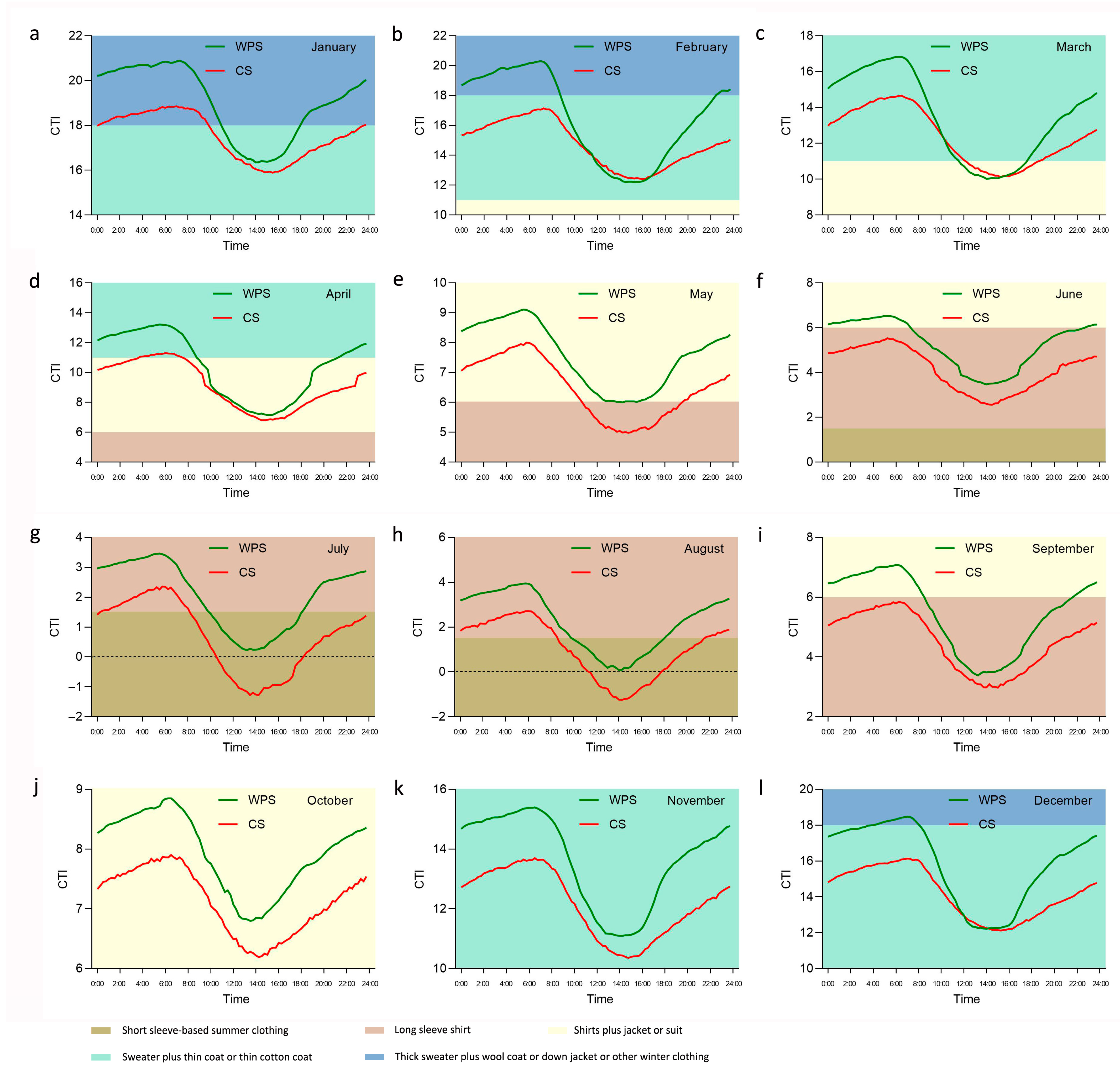
3.3.2. Daily Variation of the CTI and Clothing Suggestions

As shown in Figure 8, the daily variations of the CTI in the WPS and CS in each month demonstrated an increasing and then decreasing trend, followed by a slowly increasing trend. In February, March, and December, the CTI values in the WPS were larger than those in the CS in certain time periods (Figure 8b,c,l). Taking March for example, the CTI in the WPS was lower than that in the CS during the period of 10:15–15:30, whereas it was higher in other periods (Figure 8c). Apart from February, March, and December, the CTI values in the WPS were higher than those in the CS in all periods in all other months (Figure 8a,d–k).

Clothing suggestions are further discussed based on the daily variation of the CTI. In January, the daily variation of the CTI in both the WPS and CS was reduced from level V to level IV before increasing to level V (Figure 8a). In February, the daily variation of the CTI in the WPS reduced from level V to level IV before increasing to level V, while that in the CS stayed in level IV over the whole day (Figure 8b). In March, the daily variation of the CTI in both the WPS and CS was reduced from level IV to level III before increasing to level IV (Figure 8c). In April, the daily variation in the WPS was reduced from level IV to level III before increasing to level IV, while that in the CS increased from level III to level IV before reducing to level III (Figure 8d). In May, the WPS stayed at level III over the whole day, while that in the CS was reduced from level III to level II before increasing to level III (Figure 8e). In June and September, the daily variation of the CTI in the WPS was reduced from level III to level II before increasing to level III, while that in the CS stayed at level II over the whole day (Figure 8f,i). In July, the daily variation of the CTI in the WPS was reduced from level II to level I before increasing to level II, while that in the CS increased from level I to level II before reducing to level I (Figure 8g). In August, the daily variation of the CTI in both the WPS and CS was reduced from level II to level I before increasing to level II (Figure 8h). In October, both the WPS and CS stayed at level III over the whole day (Figure 8j). In November, both the WPS and CS stayed at level IV over the whole day (Figure 8k). Finally, in December, the daily variation of the CTI in the WPS increased from level IV to level V before reducing to level IV, while the CS stayed at level IV over the whole day (Figure 8l).

4. Discussion

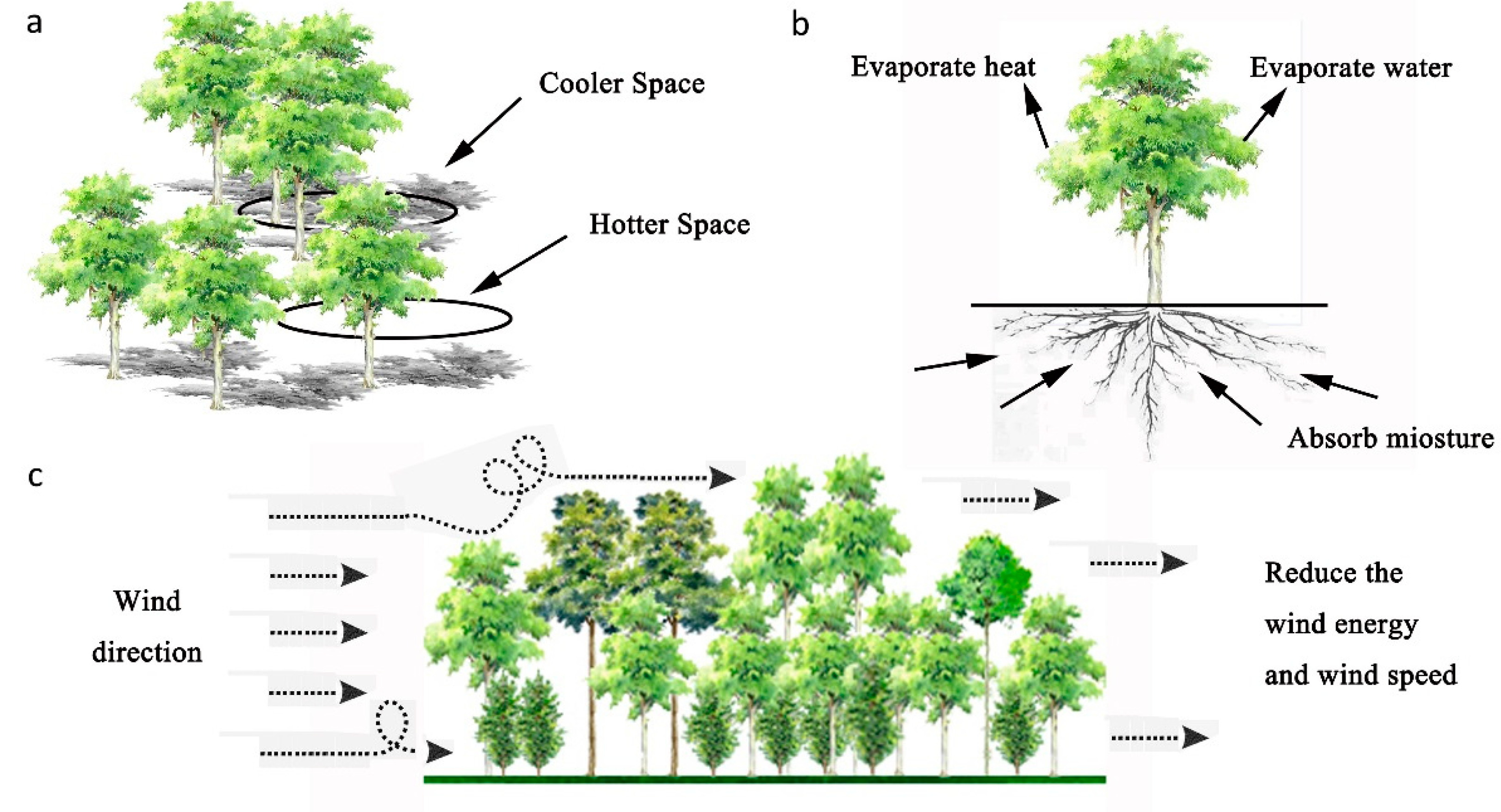
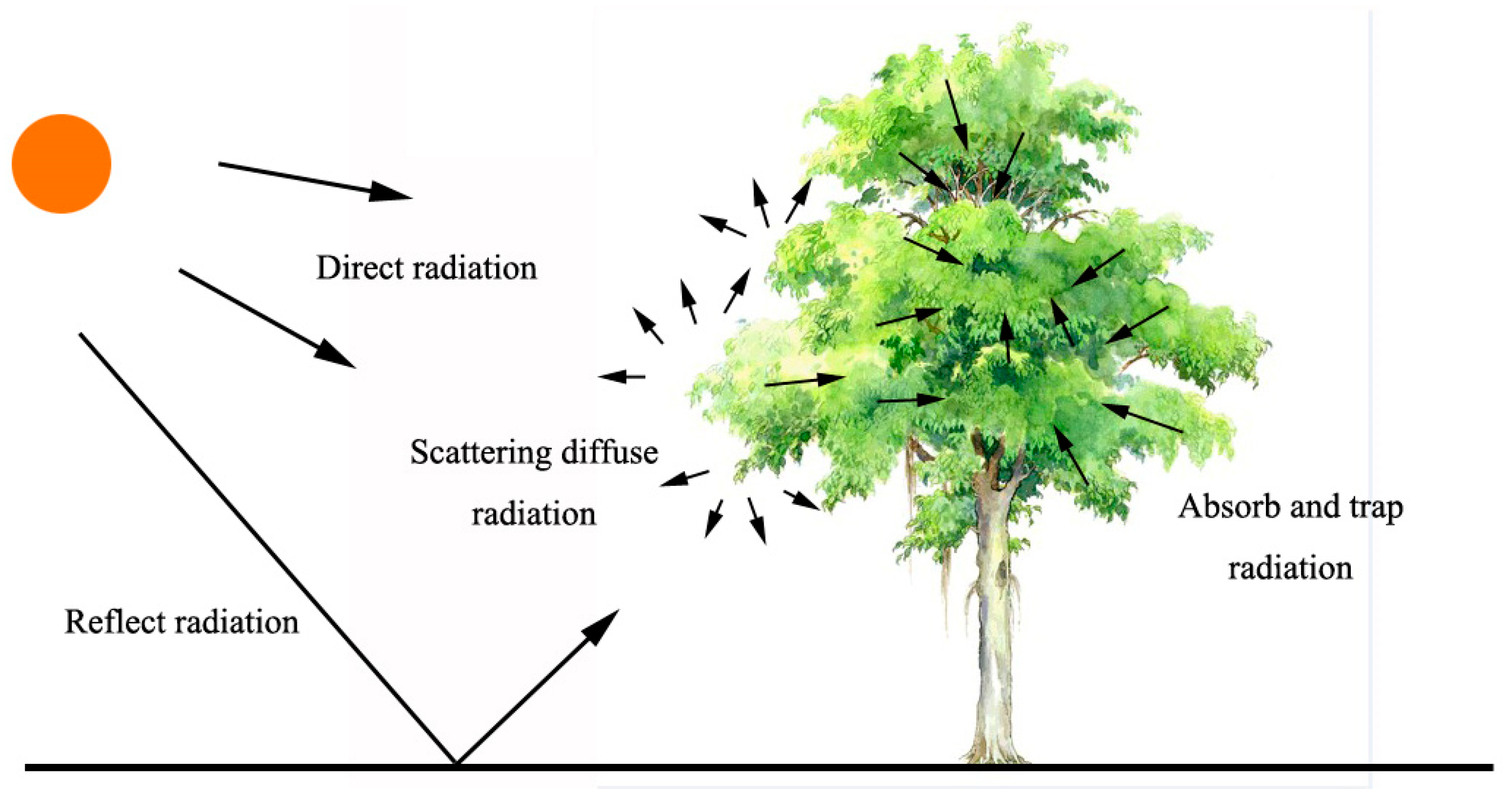
4.1. Ecosystem Services of Urban Wetland Parks in Terms of Microclimate Improvement

This study explored the microclimate and HTC of urban wetland parks, and the seasonal, monthly, and daily variations of the microclimate, HTCI, and CTI were quantitatively analyzed. The results demonstrate that the WPS displayed evident seasonal and monthly changes in the microclimate, suggesting that the microclimates of urban wetland parks are affected primarily by the overall water and heat conditions and maintain similar changes as the regional climate [44]. HTCI was studied on an annual scale, which resulted in a relatively larger range fluctuation. This phenomenon of large ranges on a larger space–time scale has been mentioned in other studies by Vinogradova (2021) [45] and An et al. (2021) [46]. Therefore, in order to obtain a perception of a certain scenario, we also mainly studied the monthly and daily variations of HTCI. The ecological benefits exhibited reduced temperature, increased humidity, and decreased wind speed in summer and other hot months, which confirms that urban wetland parks could provide good ecological services in terms of mitigating the heat island effect and dry island effect.

The findings have been supported by other studies [16,47,48,49,50]. The main reason for these is that, compared with gray infrastructure (impermeable concrete and buildings), green infrastructure, especially trees and water bodies, can absorb solar radiation, reduce the land surface temperature, and reduce the increase in vapor caused by solar radiation [17,51,52]. Moreover, ecological infrastructures that are reliant on vegetation can reduce the temperature via shading and increase heat fluxes, because they prevent the solar radiation from reaching the surface and through evapotranspiration to form low-temperature areas under canopies or in grasslands) [18,53]. Additionally, the natural branching configuration of plants can directly block the wind, produce a wind barrier effect, and can reduce the wind energy via the swinging of branches, thereby reducing wind speed (see Figure 9).

Some interesting findings based on the further analysis of the daily variation in each month were also presented. It was found that urban wetland parks have a warming effect in the midday of the cold months, while they can effectively reduce fluctuations in the daily variation of the wind speed in warmer months. The lack of vegetation and the thermal conductivity of large, impervious surfaces in urban environments result in faster heat loss during colder months [54,55,56]. Additionally, urban forests will also modify the airflow, thereby causing local strong winds, and the wind chill benefit is obvious during colder months. However, the ecological infrastructures in urban wetland parks have complex spatial structures, and therefore do not have the smooth, reflective planes of artificial facilities. Thus, when solar radiation reaches living organisms such as plants, it can be trapped by plants or diffuse, thereby affecting the energy exchange between vegetation patches [57] (see Figure 10). Moreover, the ecological infrastructures in urban wetland parks also offset a portion of the wind energy via branches and leaves, thereby reducing the daily variation of the wind speed. Therefore, urban wetland parks exert a certain heat preservation effect in the midday period of cold months, rather than a real warming effect.

4.2. HTC Features of Urban Wetland Parks

HTC is a parameter based on temperature, relative humidity, and wind. The data collected and analyzed in this study indicate that the HTCI in the WPS presented significant seasonal variation. In spring, summer, and autumn, the HTCI in the WPS was at a very comfortable and comfortable level, respectively, whereas in winter, it was at a very uncomfortable level. However, the urban wetland park was found to have a better comfort level than the urban environment only in summer (July and August).

The daily variation of the HTC in each month was also discussed. Xixi National Wetland Park can provide a comfortable environment throughout the day in May, June, July, September, and October, as well as at midday in March, April, and November. A comfortable environment was not available at noon in August or throughout the day in winter (December, January, and February). However, compared with the urban environment, Xixi National Wetland Park was found to have significantly improved comfort in the midday hours of winter.

For Hangzhou, China, which has a subtropical monsoon climate, compared with other climatic factors, humidity has a greater impact on the comfort perception of the human body throughout the year. Particularly, in winter, the “cold and wet” climate features are very unfavorable to people staying outdoors [58]. In the cooler months, urban wetland parks can increase outdoor comfort in the warm midday hours. In August, compared with the urban environment, the urban wetland park was found to provide a better comfort level in the midday hours, but the high temperature and high humidity are not sufficient to make a person feel comfortable. Hence, based on the comparison between the comfort levels provided by the urban wetland park and urban environment, in an urban wetland park with a subtropical monsoon climate, July and August provide the largest improvements of HTC.

4.3. Clothing Suggestions

According to the definition and purpose of the CTI, although Xixi National Wetland Park is in a subtropical climate area, the residents are suggested to wear heavy winter clothes when they go out in the cold season due to the restriction of high air humidity, especially at night. Recreational activities with accommodation are not recommended in winter, and specific protective measures should be taken to make visitors feel comfortable.

When visitors go to Xixi National Wetland Park in summer, they will feel much more comfortable wearing cool summer clothes. In August, they are suggested to take good protective measures (e.g., to wear a sunshade hat and sun-protective clothing) and enjoy their activities in the morning, evening, or at night, not at midday.

In this study, the HTCI and CTI were synthetically calculated by climate factors. While both indexes have had numerous applications since their conception, they both indirectly reflect the human body perception and provide clothing suggestions. Hence, in future research, determining the direct perceptions of volunteers and further combining these data with climate data to carry out an evidence-based study will be conducive to research on the relationship between the ecological environment and human health.

5. Conclusions

The increase of gray infrastructure (e.g., concrete buildings, hard pavements, and metal materials) and the decrease of ecological infrastructure (e.g., greenbelts, wetlands, and water bodies) change the underlying structure of the urban ecological environment, thereby affecting the ecosystem services in urban areas [52]. In this study, the effect of urban wetland parks on HTC over one year was quantified, and the results indicate that urban wetland parks can mitigate the heat island effect and dry island effect (by reducing the temperature, increasing the humidity, and reducing the wind speed) in summer, thereby exhibiting a good ecological function. More importantly, urban wetland parks can provide ecological services at midday during winter to mitigate the cold island effect, thereby exerting a certain heat preservation effect. Additionally, urban wetland parks were found to exhibit their best performance in improving HTC during the daytime of the hot season (June, July, August, and September, and especially the whole day in July and August) and the midday period of the cold season (December, January, February, and March). However, improvements in other months (especially in October and November) were not authenticated by the data analyzed in this study. Finally, based on the findings of this study, it is suggested that citizens should take good protective measures and enjoy their activities in the morning, evening, or at night, not at midday in hot weather. Moreover, extra layers are suggested to be worn before visiting urban wetland parks at night in cold weather, and recreational activities involving accommodation are not recommended.

In urban planning, more green space (plants) and blue space (water bodies) should be introduced, and the effect of impervious surfaces on the land surface climate should be reduced to create a microclimate conducive to human health. Administrators and policymakers should consider detailed management and strategies in parks and should plan indoor and outdoor activities for visitors to induce the most comfort and relaxation.

Finally, the HTCI is based upon a thermal stress index that does not account for radiation, which is difficult to comprehensively characterize from a microclimatic perspective. Meanwhile, like other empirical indexes, the HTCI is also intrinsically unable to take into account metabolic rate and clothing insulation. These are the certain limitations of this study. In addition, because each thermal index has its own applicable scope, it is suggested that, in addition to focusing on the research object and its thermal environment condition, the selection of the index and the formulation of a monitoring program should take into account the clothing insulation effect, metabolic activity changes, and the spatial heterogeneity of temperature [37].

References

1. Lai, D.; Zhou, C.; Huang, J.; Jiang, Y.; Long, Z.; Chen, Q. Outdoor space quality: A field study in an urban residential community in central China. Energy Build. 2014, 68, 713–720. [Google Scholar] [CrossRef]
2. Schinasi, L.H.; Benmarhnia, T.; De Roos, A.J. Modification of the association between high ambient temperature and health by urban microclimate indicators: A systematic review and meta-analysis. Environ. Res. 2018, 161, 168–180. [Google Scholar] [CrossRef]
3. Tsavdaroglou, M.; Al-Jibouri, S.H.; Bles, T.; Halman, J.I. Proposed methodology for risk analysis of interdependent critical infrastructures to extreme weather events. Int. J. Crit. Infrastruct. Prot. 2018, 21, 57–71. [Google Scholar] [CrossRef]
4. Wazneh, H.; Arain, M.A.; Coulibaly, P. Climate indices to characterize climatic changes across southern Canada. Meteorol. Appl. 2019, 27, e1861. [Google Scholar] [CrossRef] [Green Version]
5. Mitchell, M.G.E.; Suarez-Castro, A.F.; Martinez-Harms, M.; Maron, M.; McAlpine, C.; Gaston, K.J.; Johansen, K.; Rhodes, J.R. Reframing landscape fragmentation’s effects on ecosystem services. Trends Ecol. Evol. 2015, 30, 190–198. [Google Scholar] [CrossRef] [PubMed] [Green Version]
6. Wlemm, K.; Heusinkvseld, B.G.; Lenzholzer, S.; Hove, B. Street greenery and its physical and psychological impact on thermal comfort. Landsc. Urban Plan. 2015, 138, 87–98. [Google Scholar]
7. Mei, Y.; Sohngen, B.; Babb, T. Valuing urban wetland quality with hedonic price model. Ecol. Indic. 2018, 84, 535–545. [Google Scholar] [CrossRef]
8. Bertassello, L.E.; Rao, P.S.C.; Park, J.; Jawitz, J.W.; Botter, G. Stochastic modeling of wetland-groundwater systems. Adv. Water Resour. 2018, 112, 214–223. [Google Scholar] [CrossRef]
9. Park, J.; Wang, D.; Kumar, M. Spatial and temporal variations in the groundwater contributing areas of inland wetlands. Hydrol. Process. 2019, 34, 1117–1130. [Google Scholar] [CrossRef]
10. Gutzwiller, K.J.; Flather, C. Wetland features and landscape context predict the risk of wetland habitat loss. Ecol. Appl. 2011, 21, 968–982. [Google Scholar] [CrossRef]
11. Herbert, E.R.; Boon, P.; Burgin, A.J.; Neubauer, S.; Franklin, R.; Ardon, M.; Hopfensperger, K.N.; Lamers, L.P.M.; Gell, P. A global perspective on wetland salinization: Ecological consequences of a growing threat to freshwater wetlands. Ecosphere 2015, 6, art206. [Google Scholar] [CrossRef]
12. Li, N.; Tian, X.; Li, Y.; Fu, H.; Jia, X.; Jin, G.; Jiang, M. Seasonal and Spatial Variability of Water Quality and Nutrient Removal Efficiency of Restored Wetland: A Case Study in Fujin National Wetland Park, China. Chin. Geogr. Sci. 2018, 28, 1027–1037. [Google Scholar] [CrossRef] [Green Version]
13. Vanos, J.K.; Warland, J.S.; Gillespie, T.J.; Kenny, N.A. Review of the physiology of human thermal comfort while exercising in urban landscapes and implications for bioclimatic design. Int. J. Biometeorol. 2010, 54, 319–334. [Google Scholar] [CrossRef] [PubMed]
14. Cheng, X.; Yang, L.; Cao, J.; Liang, D.; Song, G. Knowledge Mapping on Literature Research Progress of Human Thermal Comfort in buildings Based on Web of Science. IOP Conf. Ser. Earth Environ. Sci. 2020, 514. [Google Scholar] [CrossRef]
15. Blazejczyk, K.; Epstein, Y.; Jendritzky, G.; Staiger, H.; Tinz, B. Comparison of UTCI to selected thermal indices. Int. J. Biometeorol. 2011, 56, 515–535. [Google Scholar] [CrossRef] [PubMed] [Green Version]
16. Mughal, M.O.; Kubilay, A.; Fatichi, S.; Meili, N.; Carmeliet, J.; Edwards, P.; Burlando, P. Detailed investigation of microclimate by means of computational fluid dynamics (CFD) in a tropical urban environment. Urban Clim. 2021, 39, 10093. [Google Scholar] [CrossRef]
17. Meili, N.; Manoli, G.; Burlando, P.; Carmeliet, J.; Chow, W.T.L.; Coutts, A.M.; Roth, M.; Velasco, E.; Vivoni, E.R.; Fatichi, S. Tree effects on urban microclimate: Diurnal, seasonal, and climatic temperature differences explained by separating radiation, evapotranspiration, and roughness effects. Urban For. Urban Green. 2021, 58, 126970. [Google Scholar] [CrossRef]
18. Meili, N.; Acero, J.A.; Peleg, N.; Manoli, G.; Burlando, P.; Fatichi, S. Vegetation cover and plant-trait effects on outdoor thermal comfort in a tropical city. Build. Environ. 2021, 195, 107733. [Google Scholar] [CrossRef]
19. Lai, D.; Guo, D.; Hou, Y.; Lin, C.; Chen, Q. Studies of outdoor thermal comfort in northern China. Build. Environ. 2014, 77, 110–118. [Google Scholar] [CrossRef]
20. Chatzidimitriou, A.; Yannas, S. Microclimate development in open urban spaces: The influence of form and materials. Energy Build. 2015, 108, 156–174. [Google Scholar] [CrossRef]
21. Estoque, R.C.; Murayama, Y.; Myint, S.W. Effects of landscape composition and pattern on land surface temperature: An urban heat island study in the megacities of Southeast Asia. Sci. Total. Environ. 2017, 577, 349–359. [Google Scholar] [CrossRef] [PubMed]
22. Yang, B.; Olofsson, T.; Nair, G.; Kabanshi, A. Outdoor thermal comfort under subarctic climate of north Sweden—A pilot study in Umeå. Sustain. Cities Soc. 2017, 28, 387–397. [Google Scholar] [CrossRef]
23. Zhao, Q.; Sailor, D.J.; Wentz, E.A. Impact of tree locations and arrangements on outdoor microclimates and human thermal comfort in an urban residential environment. Urban For. Urban Green. 2018, 32, 81–91. [Google Scholar] [CrossRef] [Green Version]
24. Pan, L.; Cui, L.; Wu, M. Tourist behaviors in wetland park: A preliminary study in Xixi National Wetland Park, Hangzhou, China. Chin. Geogr. Sci. 2010, 20, 66–73. [Google Scholar] [CrossRef]
25. Steadman, R.G. The assessment of sultriness. Part I: A temperature-humidity index based on human physiology and clothing science. J. Appl. Meteorol. 1979, 18, 861–873. [Google Scholar] [CrossRef] [Green Version]
26. Sirangelo, B.; Caloiero, T.; Coscarelli, R.; Ferrari, E.; Fusto, F. Combining stochastic models of air temperature and vapour pressure for the analysis of the bioclimatic comfort through the Humidex. Sci. Rep. 2020, 10, 11395. [Google Scholar] [CrossRef]
27. Masterton, J.M.; Richardson, F.A. Humidex: A Method of Quantifying Human Discomfort Due to Excessive Heat and Humidity; CLI1-79, Environment Canada, Atmospheric Environment: Toronto, ON, Canada, 1979. [Google Scholar]
28. Houghton, F.C.; Yaglou, C.P. Determining Equal Comfort Lines. J. Am. Soc. Heat. Vent. Eng. 1923, 29, 165–176. [Google Scholar]
29. ISO 7243. Hot environments—Estimation of the Heat Stress on Working Man, Based on the WBGT Index (Wet Bulb Globe Temperature); International Standardization Organisation: Geneva, Switzerland, 1989. [Google Scholar]
30. Alfano, F.R.D.; Palella, B.I.; Riccio, G. On the Problems Related to Natural Wet Bulb Temperature Indirect Evaluation for the Assessment of Hot Thermal Environments by Means of WBGT. Ann. Occup. Hyg. 2012, 56, 1063–1079. [Google Scholar] [CrossRef] [Green Version]
31. Lin, L.; Luo, M.; Chan, T.O.; Ge, E.; Liu, X.; Zhao, Y.; Liao, W. Effects of urbanization on winter wind chill conditions over china. Sci. Total Environ. 2019, 688, 389–397. [Google Scholar] [CrossRef] [PubMed]
32. Gagge, A.P.; Stolwijk, J.A.J.; Nishi, Y. An effective temperature scale based on a simple model of human physiological regulatory response. Ashrae Trans. 1971, 77, 21–36. [Google Scholar]
33. Gagge, A.P.; Fobelets, A.P.; Berglund, L.G. A standard predictive index of human response to the thermal environment. Ashrae Trans. 1986, 92, 709–731. [Google Scholar]
34. ISO 11079. Evaluation of Cold Environments: Determination of Required Clothing Insulation (IREQ); International Standardization Organisation: Geneva, Switzerland, 2007. [Google Scholar]
35. Alfano, F.R.D.; Palella, B.I.; Riccio, G. Notes on the implementation of the IREQ model for the assessment of extreme cold environments. Ergonomics 2013, 56, 707–724. [Google Scholar] [CrossRef] [PubMed]
36. ISO 7933. Ergonomics of the Thermal Environment: Analytical Determination and Interpretation of Heat Stress Using Calculation of the Predicted Heat Strain; International Standardization Organisation: Geneva, Switzerland, 2004. [Google Scholar]
37. Alfano, F.R.D.; Palella, B.I.; Riccio, G. Thermal Environment Assessment Reliability Using Temperature—Humidity Indices. Ind. Health 2011, 49, 95–106. [Google Scholar] [CrossRef] [PubMed] [Green Version]
38. Höppe, P. The physiological equivalent temperature—A universal index for the biometeorological assessment of the thermal environment. Int. J. Biometeorol. 1999, 43, 71–75. [Google Scholar] [CrossRef] [PubMed]
39. Jendritzky, G.; Bessemoulin, P.; Blazejczyk, K.; Cegnar, T.; Dittmann, E.; Fiala, D.; Nicol, F.; Havenith, G.; Hassi, J.; Höppe, P.; et al. Towards a Universal Thermal Climate Index UTCI for Assessing the Thermal Environment of the Human Being; Final Report COST Action 730; European Concerted Research Action: Freiburg, Germany, 2009. [Google Scholar]
40. Lu, D.; Cui, S.; Li, C. The Influence of Beijing Urban Greening and Summer Microclimate Conditions on Human Fitness; Forestry and Metrology Papers; Meteorological Press: Beijing, China, 1984; pp. 144–152. (In Chinese) [Google Scholar]
41. Gu, L.; Wang, C.; Wang, Y.; Wang, X.; Sun, Z.; Wang, Q.; Sun, R. Patterns of temporal variation of microclimate and extent of human comfort in the recreation forests in Huishan National Forest Park. Sci. Silvae Sin. 2019, 55, 150–159. (In Chinese) [Google Scholar]
42. Jin, G.; Liu, H.; Lu, Z.; Wu, J.; Xu, L.; Sun, G.; Li, P.; Li, J.; Xu, C. Canopy structures and degree of comfort with urban forests of Beijing in summer. J. Zhejiang AF Univ. 2019, 36, 550–556. (In Chinese) [Google Scholar]
43. Zhu, L.; Qian, P.; Qian, Y. Weather index study for clothing. Sci. Meteorol. Sin. 2001, 21, 468–473. (In Chinese) [Google Scholar]
44. Rapp, J.M.; Silman, M.R. Diurnal, seasonal, and altitudinal trends in microclimate across a tropical montane cloud forest. Clim. Res. 2012, 55, 17–32. [Google Scholar] [CrossRef]
45. Vinogradova, V. Using the Universal Thermal Climate Index (UTCI) for the assessment of bioclimatic conditions in Russia. Int. J. Biometeorol. 2020, 65, 1473–1483. [Google Scholar] [CrossRef]
46. An, L.; Hong, B.; Cui, X.; Geng, Y.; Ma, X. Outdoor thermal comfort during winter in China’s cold regions: A comparative study. Sci. Total Environ. 2021, 768, 144464. [Google Scholar] [CrossRef]
47. Georgi, N.J.; Zafiriadis, K. The impact of park trees on microclimate in urban areas. Urban Ecosyst. 2006, 9, 195–209. [Google Scholar] [CrossRef]
48. Wu, Z.; Chen, L. Optimizing the spatial arrangement of trees in residential neighborhoods for better cooling effects: Integrating modeling with in-situ measurements. Landsc. Urban Plan. 2017, 167, 463–472. [Google Scholar] [CrossRef]
49. Atwa, S.; Ibrahim, M.G.; Murata, R. Evaluation of plantation design methodology to improve the human thermal comfort in hot-arid climatic responsive open spaces. Sustain. Cities Soc. 2020, 59, 102198. [Google Scholar] [CrossRef]
50. Hu, L.; Li, Q. Greenspace, bluespace, and their interactive influence on urban thermal environments. Environ. Res. Lett. 2020, 15, 034041. [Google Scholar] [CrossRef]
51. Lin, Y.-H.; Tsai, K.-T. Screening of Tree Species for Improving Outdoor Human Thermal Comfort in a Taiwanese City. Sustainability 2017, 9, 340. [Google Scholar] [CrossRef] [Green Version]
52. Soydan, O. Effects of landscape composition and patterns on land surface temperature: Urban heat island case study for Nigde, Turkey. Urban Clim. 2020, 34, 100688. [Google Scholar] [CrossRef]
53. Gkatsopoulos, P. A Methodology for Calculating Cooling from Vegetation Evapotranspiration for Use in Urban Space Microclimate Simulations. Procedia Environ. Sci. 2017, 38, 477–484. [Google Scholar] [CrossRef]
54. Liu, W.; Zhang, Y.; Deng, Q. The effects of urban microclimate on outdoor thermal sensation and neutral temperature in hot-summer and cold-winter climate. Energy Build. 2016, 128, 190–197. [Google Scholar] [CrossRef]
55. Kántor, N.; Kovács, A.; Takács, Á. Seasonal differences in the subjective assessment of outdoor thermal conditions and the impact of analysis techniques on the obtained results. Int. J. Biometeorol. 2016, 60, 1615–1635. [Google Scholar] [CrossRef] [PubMed] [Green Version]
56. Yuan, C.; Adelia, A.S.; Mei, S.; He, W.; Li, X.-X.; Norford, L. Mitigating intensity of urban heat island by better understanding on urban morphology and anthropogenic heat dispersion. Build. Environ. 2020, 176, 106876. [Google Scholar] [CrossRef]
57. Gaudio, N.; Gendre, X.; Saudreau, M.; Seigner, V.; Balandier, P. Impact of tree canopy on thermal and radiative microclimates in a mixed temperate forest: A new statistical method to analyse hourly temporal dynamics. Agric. For. Meteorol. 2017, 237–238, 71–79. [Google Scholar] [CrossRef] [Green Version]
58. Peng, X.; Wu, W.; Zheng, Y.; Sun, J.; Hu, T.; Wang, P. Correlation analysis of land surface temperature and topographic elements in Hangzhou, China. Sci. Rep. 2020, 10, 1–16. [Google Scholar] [CrossRef] [PubMed]
Figure 1. The wetland park site and the control site in Hangzhou, China.
Forests 12 01322 g001
Figure 2. The seasonal, monthly, and daily variations of the average temperature in the WPS and CS. (a) The seasonal variation of the average temperature; different lowercase letters of the same color indicate results of a one-way ANOVA followed by Tukey’s test (p < 0.05), and error bars represent the standard deviation. (b) The monthly variation of the average temperature. (c) The daily variation of temperature in February. (d) The daily variation of temperature in July. Note: Significant differences between the means of WPS and CS were determined using Student’s t-test (* p < 0.05, ** p < 0.01, *** p < 0.001).
Forests 12 01322 g002
Figure 3. The seasonal, monthly, and daily variations of the average relative humidity in the WPS and CS. (a) The seasonal variation of the average relative humidity; different lowercase letters of the same color indicate results of a one-way ANOVA followed by Tukey’s test (p < 0.05), and error bars represent the standard deviation. (b) The monthly variation of the average relative humidity. (c) The daily variation of relative humidity in February. (d) The daily variation of relative humidity in August. Note: Significant differences between the means of WPS and CS were determined using Student’s t-test (*** p < 0.001).
Forests 12 01322 g003
Figure 4. The seasonal, monthly, and daily variations of the average wind speed in the WPS and CS. (a) The seasonal variation of the average wind speed; different lowercase letters of the same color indicate results of a one-way ANOVA followed by Tukey’s test (p < 0.05), and error bars represent the standard deviation. (b) The monthly variations of the average wind speed. (c) The daily variation of wind speed in February. (d) The daily variation of wind speed in August. Note: Significant differences between the means of WPS and CS were determined using Student’s t-test (*** p < 0.001).
Forests 12 01322 g004
Figure 5. The seasonal and monthly variations of the HTCI in the WPS and CS. (a) The seasonal variation of the HTCI; different lowercase letters of the same color indicate results of a one-way ANOVA followed by Tukey’s test (p < 0.05), and error bars represent the standard deviation. (b) The monthly variations of the HTCI, and error bars represent the standard deviation. Note: Significant differences between the means of WPS and CS were determined using Student’s t-test (** p < 0.01, *** p < 0.001).
Forests 12 01322 g005
Figure 6. The daily variation of the HTCI between (a) January and (l) December in the WPS and CS.
Forests 12 01322 g006
Figure 7. The seasonal and monthly variations of the CTI in the WPS and CS. (a) The seasonal variations of the CTI; different lowercase letters of the same color indicate results of a one-way ANOVA followed by Tukey’s test (p < 0.05), and error bars represent the standard deviation. (b) The monthly variations of the CTI. Significant differences between the means of WPS and CS were determined using Student’s t-test (** p < 0.01, *** p < 0.001).
Forests 12 01322 g007
Figure 8. The daily variation of the CTI between (a) January and (l) December in the WPS and CS.
Forests 12 01322 g008
Figure 9. Schematic diagrams of the (a) shading, (b) transpiration, and (c) wind barrier effects of plant communities.
Forests 12 01322 g009
Figure 10. A diagram of the absorption and diffuse reflection of solar radiation by plants.
Forests 12 01322 g010