Ecological Diversity within Rear-Edge: A Case Study from Mediterranean Quercus pyrenaica Willd.

 ,
,  , and
, and
Abstract
1. Introduction
2. Materials and Methods
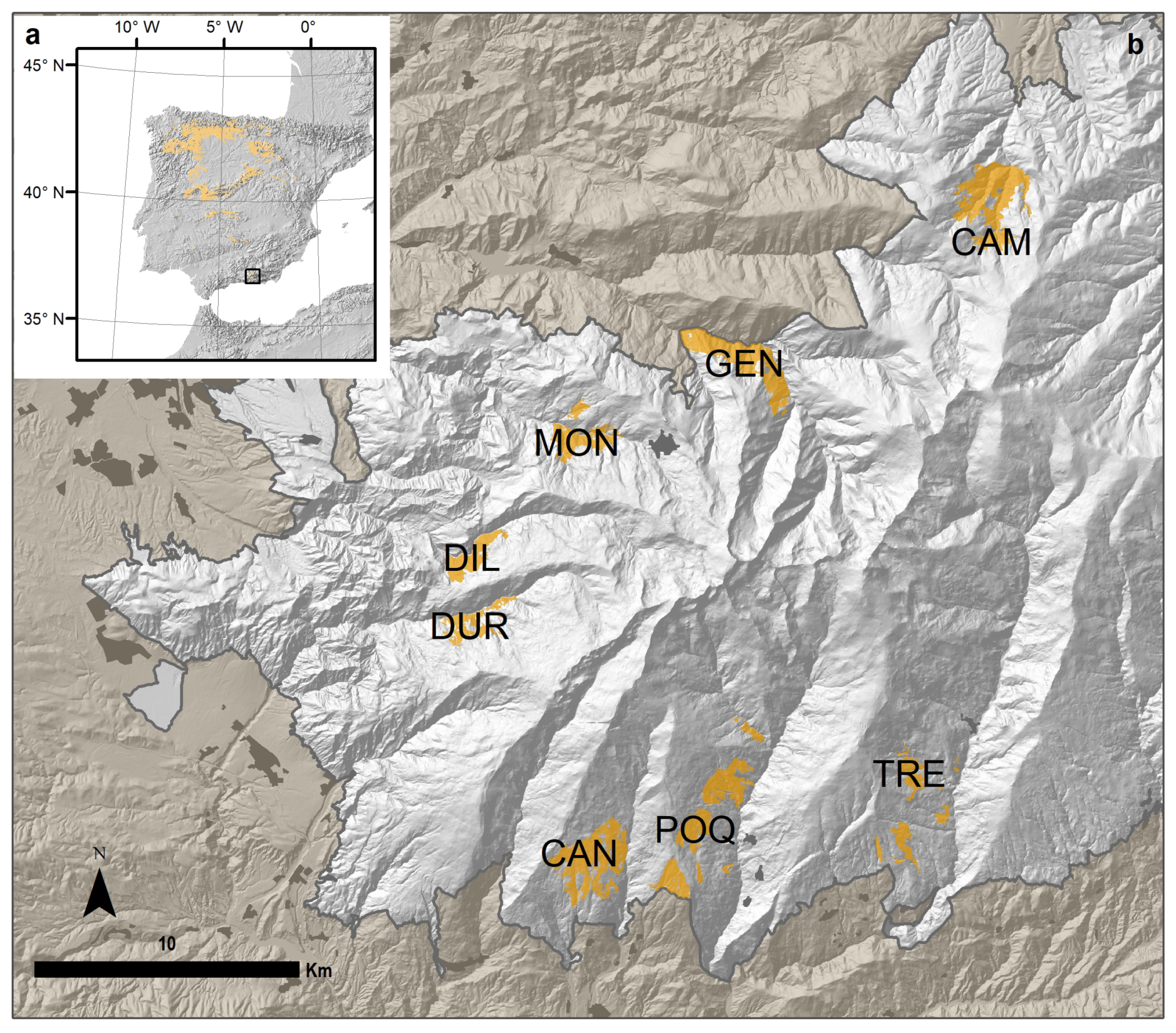
2.1. Study Area
2.2. Quercus pyrenaica Forests
2.3. Environmental Data
2.4. Forest Attributes
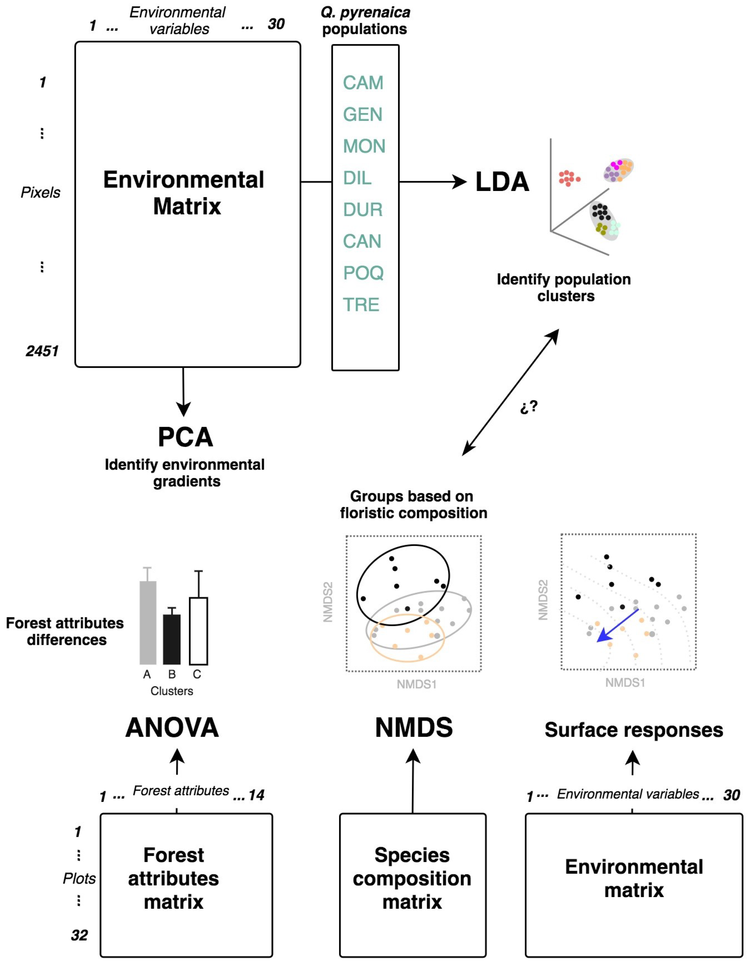
2.5. Statistical Analysis
3. Results
4. Discussion
4.1. Ecological Diversity within the Rear-Edge
4.2. The Importance of Summer Rainfall at the Micro-Habitat Level
4.3. Implications for Forecasting and Modeling
5. Conclusions: Biodiversity from the Genetics to the Landscape
Supplementary Materials
Author Contributions
Funding
Acknowledgments
Conflicts of Interest
References
- Fady, B.; Aravanopoulos, F.A.; Alizoti, P.; Mátyás, C.; von Wühlisch, G.; Westergren, M.; Belletti, P.; Cvjetkovic, B.; Ducci, F.; Huber, G.; et al. Evolution-based approach needed for the conservation and silviculture of peripheral forest tree populations. For. Ecol. Manag. 2016, 375, 66–75. [Google Scholar] [CrossRef]
- Hampe, A.; Petit, R.J. Conserving biodiversity under climate change: The rear edge matters. Ecol. Lett. 2005, 8, 461–467. [Google Scholar] [CrossRef] [PubMed]
- Castro, J.; Zamora, R.; Hódar, J.A.; Gómez, J.M. Seedling establishment of a boreal tree species (Pinus sylvestris) at its southernmost distribution limit: Consequences of being in a marginal Mediterranean habitat. J. Ecol. 2004, 92, 266–277. [Google Scholar] [CrossRef]
- Benavides, R.; Rabasa, S.G.; Granda, E.; Escudero, A.; Hódar, J.A.; Martínez-Vilalta, J.; Rincón, A.M.; Zamora, R.; Valladares, F. Direct and indirect effects of climate on demography and early growth of Pinus sylvestris at the rear edge: Changing roles of biotic and abiotic factors. PLoS ONE 2013, 8, e59824. [Google Scholar] [CrossRef]
- Gea-Izquierdo, G.; Cañellas, I. Local climate forces instability in long-term productivity of a Mediterranean oak along climatic gradients. Ecosystems 2014, 17, 228–241. [Google Scholar] [CrossRef]
- Matías, L.; Linares, J.C.; Sánchez-Miranda, A.; Jump, A.S. Contrasting growth forecasts across the geographical range of Scots pine due to altitudinal and latitudinal differences in climatic sensitivity. Glob. Chang. Biol. 2017, 23, 4106–4116. [Google Scholar] [CrossRef]
- Benito-Garzón, M.; Aĺıa, R.; Robson, T.M.; Zavala, M.A. Intra-specific variability and plasticity influence potential tree species distributions under climate change. Glob. Ecol. Biogeogr. 2011, 20, 766–778. [Google Scholar] [CrossRef]
- Gea-Izquierdo, G.; Fernández-de Uña, L.; Cañellas, I. Growth projections reveal local vulnerability of Mediterranean oaks with rising temperatures. For. Ecol. Manag. 2013, 305, 282–293. [Google Scholar] [CrossRef]
- Chen, K.; Dorado-Liñán, I.; Akhmetzyanov, L.; Gea-Izquierdo, G.; Zlatanov, T.; Menzel, A. Influence of climate drivers and the North Atlantic Oscillation on beech growth at marginal sites across the Mediterranean. Clim. Res. 2015, 66, 229–242. [Google Scholar] [CrossRef]
- Dorado-Liñán, I.; Piovesan, G.; Martínez-Sancho, E.; Gea-Izquierdo, G.; Zang, C.; Cañellas, I.; Castagneri, D.; Di Filippo, A.; Gutiérrez, E.; Ewald, J.; et al. Geographical adaptation prevails over species-specific determinism in trees’ vulnerability to climate change at Mediterranean rear-edge forests. Glob. Chang. Biol. 2019, 25, 1296–1314. [Google Scholar] [CrossRef] [PubMed]
- Pérez-Luque, A.J.; Gea-Izquierdo, G.; Zamora, R. Land-use legacies and climate change as a double challenge to oak forest resilience: Mismatches of geographical and ecological rear edges. Ecosystems 2020. [Google Scholar] [CrossRef]
- De Frenne, P.; Rodriguez-Sanchez, F.; Coomes, D.A.; Baeten, L.; Verstraeten, G.; Vellend, M.; Bernhardt-Romermann, M.; Brown, C.D.; Brunet, J.; Cornelis, J.; et al. Microclimate moderates plant responses to macroclimate warming. Proc. Natl. Acad. Sci. USA 2013, 110, 18561–18565. [Google Scholar] [CrossRef] [PubMed]
- Oldfather, M.F.; Kling, M.M.; Sheth, S.N.; Emery, N.C.; Ackerly, D.D. Range edges in heterogeneous landscapes: Integrating geographic scale and climate complexity into range dynamics. Glob. Chang. Biol. 2020, 26, 1055–1067. [Google Scholar] [CrossRef] [PubMed]
- Elsen, P.R.; Tingley, M.W. Global mountain topography and the fate of montane species under climate change. Nat. Clim. Chang. 2015, 5, 772–776. [Google Scholar] [CrossRef]
- Pironon, S.; Villellas, J.; Morris, W.F.; Doak, D.F.; García, M.B. Do geographic, climatic or historical ranges differentiate the performance of central versus peripheral populations?: The ‘centre-periphery hypothesis’: New perspectives. Glob. Ecol. Biogeogr. 2015, 24, 611–620. [Google Scholar] [CrossRef]
- Hannah, L.; Flint, L.; Syphard, A.D.; Moritz, M.A.; Buckley, L.B.; McCullough, I.M. Fine-grain modeling of species’ response to climate change: Holdouts, stepping-stones, and microrefugia. Trends Ecol. Evol. 2014, 29, 390–397. [Google Scholar] [CrossRef]
- Körner, C.; Spehn, E. A Humboldtian view of mountains. Science 2019, 365, 1061. [Google Scholar] [CrossRef]
- Spehn, E.; Korner, C. The “Mountain Laboratory”of Nature—A Largely Unexplored Mine of Information Synthesis of the Book. In Data Mining for Global Trends in Mountain Biodiversity; Spehn, E., Korner, C., Eds.; CRC Press: Boca Raton, FL, USA, 2009; pp. 165–169. [Google Scholar] [CrossRef]
- Kohler, T.; Wehrli, A.; Jurek, M. (Eds.) Mountains and Climate Change: A Global Concern; Sustainable Mountain Development Series; Centre for Development and Environment, Swiss Agency for Development and Cooperation and Geographica Bernensia: Bern, Switzerland, 2014. [Google Scholar]
- Payne, D.; Spehn, E.M.; Snethlage, M.; Fischer, M. Opportunities for research on mountain biodiversity under global change. Curr. Opin. Environ. Sustain. 2017, 29, 40–47. [Google Scholar] [CrossRef]
- Zamora, R.; Pérez-Luque, A.J.; Bonet, F.J.; Barea-Azcón, J.M.; Aspizua, R.; Sánchez-Gutiérrez, F.J.; Cano-Manuel, F.J.; Ramos-Losada, B.; Henares-Civantos, I. Global Change Impact in the Sierra Nevada Long-Term Ecological Research Site (Southern Spain). Bull. Ecol. Soc. Am. 2017, 98, 157–164. [Google Scholar] [CrossRef]
- Meineri, E.; Hylander, K. Fine-grain, large-domain climate models based on climate station and comprehensive topographic information improve microrefugia detection. Ecography 2017, 40, 1003–1013. [Google Scholar] [CrossRef]
- Franklin, J.; Davis, F.W.; Ikegami, M.; Syphard, A.D.; Flint, L.E.; Flint, A.L.; Hannah, L. Modeling plant species distributions under future climates: How fine scale do climate projections need to be? Glob. Chang. Biol. 2013, 19, 473–483. [Google Scholar] [CrossRef] [PubMed]
- Potter, K.A.; Arthur Woods, H.; Pincebourde, S. Microclimatic challenges in global change biology. Glob. Chang. Biol. 2013, 19, 2932–2939. [Google Scholar] [CrossRef] [PubMed]
- Lo, Y.H.; Blanco, J.A.; Kimmins, J.P.H. A word of caution when planning forest management using projections of tree species range shifts. For. Chron. 2010, 86, 312–316. [Google Scholar] [CrossRef]
- Lindner, M.; Maroschek, M.; Netherer, S.; Kremer, A.; Barbati, A.; Garcia-Gonzalo, J.; Seidl, R.; Delzon, S.; Corona, P.; Kolström, M.; et al. Climate change impacts, adaptive capacity, and vulnerability of European forest ecosystems. For. Ecol. Manag. 2010, 259, 698–709. [Google Scholar] [CrossRef]
- Tito, R.; Vasconcelos, H.L.; Feeley, K.J. Mountain Ecosystems as Natural Laboratories for Climate Change Experiments. Front. For. Glob. Chang. 2020, 3, 38. [Google Scholar] [CrossRef]
- Franco, A. Quercus L. In Flora Ibérica; Castroviejo, A., Laínz, M., López-González, G., Montserrat, P., Muñoz-Garmendia, F., Paiva, J., Villar, L., Eds.; Real Jardín Botánico, CSIC: Madrid, Spain, 1990; Volume 2, pp. 15–36. [Google Scholar]
- Benito-Garzón, M.; de Dios, R.S.; Ollero, H.S. Effects of climate change on the distribution of Iberian tree species. Appl. Veg. Sci. 2008, 11, 169–178. [Google Scholar] [CrossRef]
- García-Valdés, R.; Zavala, M.A.; Araújo, M.B.; Purves, D.W. Chasing a moving target: Projecting climate change-induced shifts in non-equilibrial tree species distributions. J. Ecol. 2013, 101, 441–453. [Google Scholar] [CrossRef]
- Benito, B.; Lorite, J.; Peñas, J. Simulating potential effects of climatic warming on altitudinal patterns of key species in Mediterranean-alpine ecosystems. Clim. Chang. 2011, 108, 471–483. [Google Scholar] [CrossRef]
- Benito-Garzón, M.; de Dios, R.S.; Ollero, H.S. Predictive modeling of tree species distributions on the Iberian Peninsula during the Last Glacial Maximum and Mid-Holocene. Ecography 2007, 30, 120–134. [Google Scholar] [CrossRef]
- Felicísimo, A. (Ed.) Impactos, Vulnerabilidad y Adaptación al Cambio Climático de la Biodiversidad Española. 2. Flora y Vegetación; Oficina Española de Cambio Climático, Ministerio de Medio Ambiente y Medio Rural y Marino: Madrid, Spain, 2011. [Google Scholar]
- Ruiz-Benito, P.; Lines, E.R.; Gómez-Aparicio, L.; Zavala, M.A.; Coomes, D.A. Patterns and drivers of tree mortality in iberian forests: Climatic effects are modified by competition. PLoS ONE 2013, 8, e56843. [Google Scholar] [CrossRef]
- Ruiz-Labourdette, D.; Schmitz, M.F.; Pineda, F.D. Changes in tree species composition in Mediterranean mountains under climate change: Indicators for conservation planning. Ecol. Indic. 2013, 24, 310–323. [Google Scholar] [CrossRef]
- Urbieta, I.R.; Garćıa, L.V.; Zavala, M.A.; Marañón, T. Mediterranean pine and oak distribution in southern Spain: Is there a mismatch between regeneration and adult distribution? J. Veg. Sci. 2011, 22, 18–31. [Google Scholar] [CrossRef]
- Rehm, E.M.; Olivas, P.; Stroud, J.; Feeley, K.J. Losing your edge: Climate change and the conservation value of range-edge populations. Ecol. Evol. 2015, 5, 4315–4326. [Google Scholar] [CrossRef] [PubMed]
- Blanca, G.; Cueto, M.; Martínez-Lirola, M.; Molero-Mesa, J. Threatened vascular flora of Sierra Nevada (Southern Spain). Biol. Conserv. 1998, 85, 269–285. [Google Scholar] [CrossRef]
- Lorite, J. An updated checklist of the vascular flora of Sierra Nevada (SE Spain). Phytotaxa 2016, 261, 1–57. [Google Scholar] [CrossRef]
- Pérez-Luque, A.J.; Bonet-García, F.J.; Zamora Rodríguez, R. Map of Ecosystems Types in Sierra Nevada Mountain (Southern Spain). PANGAEA. 2019. Available online: https://doi.pangaea.de/10.1594/PANGAEA.910176 (accessed on 15 March 2020). [CrossRef]
- Gómez, J.M. Spatial patterns in long-distance dispersal of Quercus ilex acorns by jays in a heterogeneous landscape. Ecography 2003, 26, 573–584. [Google Scholar] [CrossRef]
- Valbuena-Carabaña, M.; González-Martínez, S.C.; Sork, V.L.; Collada, C.; Soto, A.; Goicoechea, P.G.; Gil, L. Gene flow and hybridisation in a mixed oak forest (Quercus pyrenaica Willd. and Quercus petraea (Matts.) Liebl.) in central Spain. Heredity 2005, 95, 457–465. [Google Scholar] [CrossRef]
- Valbuena-Carabaña, M.; Gil, L. Genetic resilience in a historically profited root sprouting oak (Quercus pyrenaica Willd.) at its southern boundary. Tree Genet. Genomes 2013, 9, 1129–1142. [Google Scholar] [CrossRef]
- Gea-Izquierdo, G.; Nicault, A.; Battipaglia, G.; Dorado-Liñán, I.; Gutiérrez, E.; Ribas, M.; Guiot, J. Risky future for Mediterranean forests unless they undergo extreme carbon fertilization. Glob. Chang. Biol. 2017, 23, 2915–2927. [Google Scholar] [CrossRef]
- CMAOT. Cartografía y Evaluación de la Vegetación y Flora de los Ecosistemas Forestales de Andalucía a Escala de Detalle (1:10,000). Consejería de Medio Ambiente y Ordenación del Territorio: Sevilla, Spain, 2014. Available online: http://sl.ugr.es/0boY (accessed on 20 May 2020).
- Guisan, A.; Zimmermann, N.E. Predictive habitat distribution models in ecology. Ecol. Model. 2000, 135, 147–186. [Google Scholar] [CrossRef]
- Williams, K.J.; Belbin, L.; Austin, M.P.; Stein, J.L.; Ferrier, S. Which environmental variables should I use in my biodiversity model? Int. J. Geogr. Inf. Sci. 2012, 26, 2009–2047. [Google Scholar] [CrossRef]
- Benito, B.M.; Pérez-Pérez, R.; Reyes-Muñoz, P.S. Climate simulations. In Sierra Nevada Global-Change Observatory: Monitoring Methodologies; Aspizua, R., Barea-Azcón, J., Bonet, F., Pérez-Luque, A., Zamora, R., Eds.; Consejería de Medio Ambiente: Junta de Andalucía, Spain, 2014; pp. 30–31. [Google Scholar]
- Ninyerola, M.; Pons, X.; Roure, J.M. A methodological approach of climatological modeling of air temperature and precipitation through GIS techniques. Int. J. Climatol. 2000, 20, 1823–1841. [Google Scholar] [CrossRef]
- Neteler, M.; Bowman, M.H.; Landa, M.; Metz, M. GRASS GIS: A multi-purpose open source GIS. Environ. Model. Softw. 2012, 31, 124–130. [Google Scholar] [CrossRef]
- Šúri, M.; Hofierka, J. A New GIS-based Solar Radiation Model and Its Application to Photovoltaic Assessments. Trans. GIS 2004, 8, 175–190. [Google Scholar] [CrossRef]
- Guisan, A.; Weiss, S.B.; Weiss, A.D. GLM versus CCA spatial modeling of plant species distribution. Plant Ecol. 1999, 143, 107–122. [Google Scholar] [CrossRef]
- Pérez-Luque, A.J.; Bonet, F.J.; Pérez-Pérez, R.; Aspizua, R.; Lorite, J.; Zamora, R. Sinfonevada: Dataset of floristic diversity in Sierra Nevada forests (SE Spain). PhytoKeys 2014, 35, 1–15. [Google Scholar] [CrossRef][Green Version]
- McElhinny, C.; Gibbons, P.; Brack, C.; Bauhus, J. Forest and woodland stand structural complexity: Its definition and measurement. For. Ecol. Manag. 2005, 218, 1–24. [Google Scholar] [CrossRef]
- Del Río, M.; Pretzsch, H.; Alberdi, I.; Bielak, K.; Bravo, F.; Brunner, A.; Condés, S.; Ducey, M.J.; Fonseca, T.; von Lüpke, N.; et al. Characterization of the structure, dynamics, and productivity of mixed-species stands: Review and perspectives. Eur. J. For. Res. 2016, 135, 23–49. [Google Scholar] [CrossRef]
- Braun-Blanquet, J. Pflanzensoziologie: Grundzuge der Vegetationskunde; Springer: Wien, Austria, 1964. [Google Scholar]
- Krebs, C.J. Ecological Methodology, 2nd ed.; Benjamin/Cummings: Menlo Park, CA, USA, 1999. [Google Scholar]
- Del Río, M.; Montes, F.; Cañellas, I.; Montero, G. Indices of stand structural diversity. For. Syst. 2003, 12, 159–176. [Google Scholar] [CrossRef]
- Dziuban, C.D.; Shirkey, E.C. When is a correlation matrix appropriate for factor analysis? Some decision rules. Psychol. Bull. 1974, 81, 358–361. [Google Scholar] [CrossRef]
- Guttman, L. Some necessary conditions for common-factor analysis. Psychometrika 1954, 19, 149–161. [Google Scholar] [CrossRef]
- Legendre, P.; Legendre, L.F. Numerical Ecology; Elsevier: Amsterdam, The Netherlands, 2012; Volume 24. [Google Scholar]
- Williams, B.K. Some observations of the use of discriminant analysis in ecology. Ecology 1983, 64, 1283–1291. [Google Scholar] [CrossRef]
- Kruskal, J.B. Nonmetric multidimensional scaling: A numerical method. Psychometrika 1964, 29, 115–129. [Google Scholar] [CrossRef]
- Minchin, P.R. Simulation of multidimensional community patterns: Towards a comprehensive model. Vegetatio 1987, 71, 145–156. [Google Scholar] [CrossRef]
- Oksanen, J. Multivariate Analysis of Ecological Communities in R: Vegan Tutorial. 2015. Available online: https://www.mooreecology.com/uploads/2/4/2/1/24213970/vegantutor.pdf (accessed on 15 March 2020).
- Virtanen, R.; Oksanen, J.; Oksanen, L.; Razzhivin, V.Y. Broad-scale vegetation-environment relationships in Eurasian high-latitude areas. J. Veg. Sci. 2006, 17, 519–528. [Google Scholar] [CrossRef]
- R Core Team. R: A Language and Environment for Statistical Computing; R Foundation for Statistical Computing: Vienna, Austria, 2019; Available online: https://www.r-project.org/ (accessed on 15 March 2019).
- Venables, W.N.; Ripley, B.D. Modern Applied Statistics with S, 4th ed.; Springer: New York, NY, USA, 2002; ISBN 0-387-95457-0. [Google Scholar]
- Raiche, G.; Magis, D. nFactors: Parallel Analysis and Other Non Graphical Solutions to the Cattell Scree Test. R Package Version 2.4.1. 2020. Available online: https://CRAN.R-project.org/package=nFactors (accessed on 15 March 2020).
- Oksanen, J.; Blanchet, F.G.; Friendly, M.; Kindt, R.; Legendre, P.; McGlinn, D.; Minchin, P.R.; O’Hara, R.B.; Simpson, G.L.; Solymos, P.; et al. Vegan: Community Ecology Package. R Package Version 2.5–6. 2019. Available online: https://CRAN.R-project.org/package=vegan (accessed on 15 March 2019).
- Friendly, M.; Fox, J. Candisc: Visualizing Generalized Canonical Discriminant and Canonical Correlation Analysis. R Package Version 0.8–3. 2020. Available online: https://CRAN.R-project.org/package=candisc (accessed on 15 March 2020).
- Murdoch, D.; Chow, E.D. Ellipse: Functions for Drawing Ellipses and Ellipse-Like Confidence Regions. R Package Version 0.4.2. 2020. Available online: https://CRAN.R-project.org/package=ellipse (accessed on 15 March 2020).
- Kassambara, A. ggpubr: ‘ggplot2’ Based Publication Ready Plots. R Package Version 0.4.0. 2020. Available online: https://CRAN.R-project.org/package=ggpubr (accessed on 15 March 2020).
- Beck, M.W. ggord: Ordination Plots with ggplot2. R Package Version 1.1.5. 2020. Available online: https://fawda123.github.io/ggord/ (accessed on 15 March 2020).
- Kassambara, A.; Mundt, F. factoextra: Extract and Visualize the Results of Multivariate Data Analyses. R Package Version 1.0.7. 2020. Available online: https://CRAN.R-project.org/package=factoextra (accessed on 15 March 2020).
- Pedersen, T.L. Patchwork: The Composer of Plots. R Package Version 1.0.1. 2020. Available online: https://CRAN.R-project.org/package=patchwork (accessed on 15 March 2020).
- Dionisio, M.A.; Alcaraz-Segura, D.; Cabello, J. Satellite-Based Monitoring of Ecosystem Functioning in Protected Areas: Recent Trends in the Oak Forests (Quercus pyrenaica Willd.) of Sierra Nevada (Spain). Int. Perspect. Global Environ. Chang. 2012, 355–374. [Google Scholar] [CrossRef]
- Pérez-Luque, A.; Pérez-Pérez, R.; Bonet-García, F.; Magaña, P. An ontological system based on MODIS images to assess ecosystem functioning of Natura 2000 habitats: A case study for Quercus pyrenaica forests. Int. J. Appl. Earth Obs. Geoinf. 2015, 37, 142–151. [Google Scholar] [CrossRef]
- Alcaraz-Segura, D.; Reyes, A.; Cabello, J. Changes in vegetation productivity according to teledetection. In Global Change Impacts in Sierra Nevada: Challenges for Conservation; Zamora, R., Pérez-Luque, A., Bonet, F., Barea-Azcón, J., Aspizua, R., Eds.; Consejería de Medio Ambiente y Ordenación del Territorio: Junta de Andalucía, Spain, 2016; pp. 142–145. [Google Scholar]
- Lorite, J.; Salazar, C.; Peñast, J.; Valle, F. Phytosociological review on the forests of Quercus pyrenaica Willd. Acta Bot. Gall. 2008, 155, 219–233. [Google Scholar] [CrossRef][Green Version]
- Gavilán, R.G.; Escudero, A.; Rubio, A. Effects of disturbance on floristic patterns of Quercus pyrenaica forests in Central Spain. In Vegetation Science in Retrospect and Perspective—Proceedings 41st IAVS Symposium; Opulus Press: Uppsala, Sweden, 2000; pp. 226–229. [Google Scholar]
- Jiménez Olivencia, Y. Los Paisajes de Sierra Nevada: Cartografía de los Sistemas Naturales de una Montaña Mediterránea; Universidad de Granada: Granada, Spain, 1991. [Google Scholar]
- Camacho-Olmedo, M.; García-Martínez, P.; Jiménez-Olivencia, Y.; Menor-Toribio, J.; Paniza-Cabrera, A. Dinámica evolutiva del paisaje vegetal de la Alta Alpujarra granadina en la segunda mitad del s. XX. Cuad. Geográficos 2002, 32, 25–42. [Google Scholar]
- Al Aallali, A.; López-Nieto, J.M.; Pérez-Raya, F.; Molero-Mesa, J. Estudio de la vegetación forestal en la vertiente sur de Sierra Nevada (Alpujarra Alta granadina). Itinera Geobot. 1998, 11, 387–402. [Google Scholar]
- Valbuena-Carabaña, M.; Gil, L. Centenary coppicing maintains high levels of genetic diversity in a root resprouting oak (Quercus pyrenaica Willd.). Tree Genet. Genomes 2017, 13, 28. [Google Scholar] [CrossRef]
- Valbuena-Carabaña, M.; Gil, L. Evaluación de la estructura genética de poblaciones marginales de Quercus Pyrenaica Willd. y su evolución. Implicaciones para la conservación de sus recursos genéticos. In Proyectos de Investigación en Parques Nacionales, 2007–2010; Ramírez, L., Asensio, B., Eds.; Naturaleza y Parques Nacionales; Serie Investigación en la Red; Organismo Autónomo Parques Nacionales: Madrid, Spain, 2011; pp. 175–204. [Google Scholar]
- Médail, F.; Diadema, K. Glacial refugia influence plant diversity patterns in the Mediterranean Basin. J. Biogeogr. 2009, 36, 1333–1345. [Google Scholar] [CrossRef]
- Gómez, A.; Lunt, D.H. Refugia within Refugia: Patterns of Phylogeographic Concordance in the Iberian Peninsula. In Phylogeography of Southern European Refugia; Weiss, S., Ferrand, N., Eds.; Springer: Dordrecht, The Netherlands, 2007; pp. 155–188. [Google Scholar] [CrossRef]
- Blanco-Pastor, J.L.; Fernández-Mazuecos, M.; Coello, A.J.; Pastor, J.; Vargas, P. Topography explains the distribution of genetic diversity in one of the most fragile European hotspots. Divers. Distrib. 2019, 25, 74–89. [Google Scholar] [CrossRef]
- Brewer, S.; Cheddadi, R.; de Beaulieu, J.L.; Reille, M. The spread of deciduous Quercus throughout Europe since the last glacial period. For. Ecol. Manag. 2002, 156, 27–48. [Google Scholar] [CrossRef]
- Olalde, M.; Herrán, A.; Espinel, S.; Goicoechea, P.G. White oaks phylogeography in the Iberian Peninsula. For. Ecol. Manag. 2002, 156, 89–102. [Google Scholar] [CrossRef]
- Rodríguez-Sánchez, F.; Hampe, A.; Jordano, P.; Arroyo, J. Past tree range dynamics in the Iberian Peninsula inferred through phylogeography and palaeodistribution modeling: A review. Rev. Palaeobot. Palynol. 2010, 162, 507–521. [Google Scholar] [CrossRef]
- Petit, R.J.; Brewer, S.; Bordacs, S.; Burg, K.; Cheddadi, R.; Coart, E.; Cottrell, J.; Csaikl, U.M.; van Dam, B.; Deans, J.D.; et al. Identification of refugia and post-glacial colonisation routes of European white oaks based on chloroplast DNA and fossil pollen evidence. For. Ecol. Manag. 2002, 156, 26. [Google Scholar] [CrossRef]
- Bhagwat, S.A.; Willis, K.J. Species persistence in northerly glacial refugia of Europe: A matter of chance or biogeographical traits? J. Biogeogr. 2008, 35, 464–482. [Google Scholar] [CrossRef]
- Birks, H.J.B.; Willis, K.J. Alpines, trees, and refugia in Europe. Plant Ecol. Divers. 2008, 1, 147–160. [Google Scholar] [CrossRef]
- Gavin, D.G.; Fitzpatrick, M.C.; Gugger, P.F.; Heath, K.D.; Rodríguez-Sánchez, F.; Dobrowski, S.Z.; Hampe, A.; Hu, F.S.; Ashcroft, M.B.; Bartlein, P.J.; et al. Climate refugia: Joint inference from fossil records, species distribution models and phylogeography. New Phytol. 2014, 204, 37–54. [Google Scholar] [CrossRef]
- Blanco Castro, E.; Costa-Tenorio, M.; Morla y Juaristi, C.; Sanz-Ollero, H. Los Bosques ibéricos: Una Interpretación Geobotánica; Planeta: Barcelona, Spain, 2005. [Google Scholar]
- García, I.; Jiménez, P. 9230 Robledales de Quercus pyrenaica y robledales de Quercus robur y Quercus pyrenaica del noroeste ibérico. In Bases Ecológicas Preliminares Para la Conservación de los Tipos de Hábitat de Interés Comunitario en España; Ministerio de Medio Ambiente, y Medio Rural y Marino: Madrid, Spain, 2009; pp. 1–66. [Google Scholar]
- del Río, S.; Herrero, L.; Penas, A. Bioclimatic analysis of the Quercus pyrenaica forests in Spain. Phytocoenologia 2007, 37, 541–560. [Google Scholar] [CrossRef]
- Gavilán, R.G.; Mata, D.S.; Vilches, B.; Entrocassi, G. Modelling current distribution of Spanish Quercus Pyrenaica Forests Using Climatic Parameters. Phytocoenologia 2007, 37, 561–581. [Google Scholar] [CrossRef]
- Pereira, P.; Oliva, M.; Misiune, I. Spatial interpolation of precipitation indexes in Sierra Nevada (Spain): Comparing the performance of some interpolation methods. Theor. Appl. Climatol. 2016, 126, 683–698. [Google Scholar] [CrossRef]
- Martínez-Parras, J.M.; Molero-Mesa, J. Ecología y fitosociología de Quercus Pyrenaica Willd. En La Prov. Bética. Los Melojares Béticos Y Sus Etapas De Sustitución. Lazaroa 1982, 4, 91–104. [Google Scholar]
- Gómez, J. Impact of vertebrate acorn- and seedling-predators on a Mediterranean Quercus pyrenaica forest. For. Ecol. Manag. 2003, 180, 125–134. [Google Scholar] [CrossRef]
- Gómez-Aparicio, L.; Pérez-Ramos, I.M.; Mendoza, I.; Matías, L.; Quero, J.L.; Castro, J.; Zamora, R.; Marañón, T. Oak seedling survival and growth along resource gradients in Mediterranean forests: Implications for regeneration in current and future environmental scenarios. Oikos 2008, 117, 1683–1699. [Google Scholar] [CrossRef]
- Mendoza, I.; Zamora, R.; Castro, J. A seeding experiment for testing tree-community recruitment under variable environments: Implications for forest regeneration and conservation in Mediterranean habitats. Biol. Conserv. 2009, 142, 1491–1499. [Google Scholar] [CrossRef]
- Gómez, J.; Gómez-Aparicio, L.; Zamora, R.; Montes, J. Problemas de Regeneración de Especies Forestales Autóctonas en el Espacio Natural Protegido de Sierra Nevada; Sociedad Española de Ciencias Forestales: Granada, Spain, 2001. [Google Scholar]
- Guisan, A.; Thuiller, W. Predicting species distribution: Offering more than simple habitat models. Ecol. Lett. 2005, 8, 993–1009. [Google Scholar] [CrossRef]
- Urbieta, I.R.; Pérez-Ramos, I.M.; Zavala, M.A.; Marañón, T.; Kobe, R.K. Soil water content and emergence time control seedling establishment in three co-occurring Mediterranean oak species. Can. J. For. Res. 2008, 38, 2382–2393. [Google Scholar] [CrossRef]
- Sánchez de Dios, R.; Benito-Garzón, M.; Sainz-Ollero, H. Present and future extension of the Iberian submediterranean territories as determined from the distribution of marcescent oaks. Plant Ecol. 2009, 204, 189–205. [Google Scholar] [CrossRef]
- López-Tirado, J.; Hidalgo, P.J. A high resolution predictive model for relict trees in the Mediterranean-mountain forests (Pinus sylvestris L., P. nigra Arnold and Abies pinsapo Boiss.) from the south of Spain: A reliable management tool for reforestation. For. Ecol. Manag. 2014, 330, 105–114. [Google Scholar] [CrossRef]
- Navarro-González, I.; Pérez-Luque, A.J.; Bonet, F.J.; Zamora, R. The weight of the past: Land-use legacies and recolonization of pine plantations by oak trees. Ecol. Appl. 2013, 23, 1267–1276. [Google Scholar] [CrossRef] [PubMed]
- Jump, A.S.; Cavin, L.; Hunter, P.D. Monitoring and managing responses to climate change at the retreating range edge of forest trees. J. Environ. Monit. 2010, 12, 1791–1798. [Google Scholar] [CrossRef] [PubMed]
- Hampe, A.; Jump, A.S. Climate Relicts: Past, Present, Future. Annu. Rev. Ecol. Evol. Syst. 2011, 42, 313–333. [Google Scholar] [CrossRef]


| Oak Population | Code | River Valley | Municipalities | Elevation (m) | Latitude | Longitude | Area (ha) |
|---|---|---|---|---|---|---|---|
| El Camarate | CAM | Alhama | Lugros | 1740 (1441–2026) | 37°10′29.49″ N | 3°15′24.33″ W | 457.15 |
| Robledal de San Juan | GEN | Genil | Güejar-Sierra | 1519 (1189–1899) | 37°7′29.63″ N | 3°21′54.60″ W | 395.00 |
| Loma de la Perdíz | MON | Monachil | Monachil | 1780 (1564–1990) | 37°5′54.87″ N | 3°25′46.65″ W | 204.55 |
| Umbría de la Dehesa de Dílar | DIL | Dílar | Dílar | 1764 (1478–1960) | 37°3′33.61″ N | 3°28′29.07″ W | 154.07 |
| Loma de Enmedio | DUR | Dúrcal | Dúrcal | 1824 (1530–2035) | 37°1′58.75″ N | 3°28′38.44″ W | 137.04 |
| El Robledal de Cáñar | CAN | Chico | Cáñar | 1687 (1366–1935) | 36°57′28.04″ N | 3°25′57.10″ W | 436.20 |
| Loma de la Matanza y Loma de Ramón | POQ | Poqueira | Soportújar, Pampaneira, Bubión, Capileira | 1740 (1214–1981) | 36°57′58.90″ N | 3°22′55.12″ W | 458.95 |
| Loma de los Lotes | TRE | Trevélez | Pórtugos, Busquístar | 1692 (1312–1963) | 36°58′37.38″ N | 3°17′25.75″ W | 197.92 |
| Code | Description | Units |
|---|---|---|
| Climate | ||
| precYE | Annual precipitation | mm |
| precSU | Summer precipitation | mm |
| precAU | Autumn precipitation | mm |
| precWI | Winter precipitation | mm |
| precSP | Spring precipitation | mm |
| tmaxSU | Summer mean maximum temperature | °C |
| tmaxAU | Autumn mean maximum temperature | °C |
| tmaxWI | Winter mean maximum temperature | °C |
| tmaxSP | Spring mean maximum temperature | °C |
| tminSU | Summer mean minimum temperature | °C |
| tminAU | Autumn mean minimum temperature | °C |
| tminWI | Winter mean minimum temperature | °C |
| tminSP | Spring mean minimum temperature | °C |
| Landscape | ||
| human | Anthropogenic influence | cells |
| Topography | ||
| elev | Elevation | meter |
| aspect | Aspect | ° |
| slope | Slope | ° |
| tpNS | North-South gradient | % |
| tpEW | East-West gradient | % |
| radSU | Summer direct radiation | Wh/m2 |
| radAU | Autumn direct radiation | Wh/m2 |
| radWI | Winter direct radiation | Wh/m2 |
| radSP | Spring direct radiation | Wh/m2 |
| radhSU | Mean duration of insolation in Summer | hour |
| radhAU | Mean duration of insolation in Autumn | hour |
| radhWI | Mean duration of insolation in Winter | hour |
| radhSP | Mean duration of insolation in Spring | hour |
| twi | Topographic wetness index | |
| tpos | Topographic position | meter |
| flow | Flow accumulation | |
| Forest biodiversity | ||
| diver | Plant diversity | |
| rich | Richness | species number |
| regTot | Total regeneration | total seedling number |
| Forest function | ||
| regQp | Pyrenean Oak regeneration | seedling number |
| regQi | Holm Oak regeneration | seedling number |
| FCC | Forest canopy cover | % |
| Forest structure | ||
| FCCTree | Forest canopy cover of Tree | % |
| FCCShru | Forest canopy cover of Shrub | % |
| FCCHerb | Forest canopy cover of Herbaceous | % |
| CCshann | Canopy Cover diversity | |
| heiTree | Tree Height | m |
| denTree | Density | trees/ha |
| BA | Basal area | m2/ha |
| vol | Volume | m3 × ha−1 |
| Variable | PC1 Load | PC1 cor. | PC2 Load | PC2 cor. | PC3 Load | PC3 cor. | LDA 1 | LDA 2 | LDA 3 |
|---|---|---|---|---|---|---|---|---|---|
| Topography | |||||||||
| twi | −0.022 | −0.069 | −0.010 | −0.024 | 0.023 | 0.046 | −0.009 | 0.005 | 0.018 |
| flow | 0.024 | 0.073 | 0.011 | 0.026 | −0.008 | −0.015 | 0.004 | −0.003 | 0.005 |
| elev | −0.158 | −0.489 | −0.016 | −0.035 | 0.142 | 0.280 | 0.000 | −0.014 | 0.105 |
| slope | 0.222 | 0.690 | −0.068 | −0.155 | 0.157 | 0.309 | 0.032 | 0.034 | −0.073 |
| tpos | −0.163 | −0.507 | −0.019 | −0.042 | −0.043 | −0.085 | −0.021 | −0.013 | 0.006 |
| aspect | −0.210 | −0.650 | −0.012 | −0.026 | −0.087 | −0.172 | −0.044 | −0.043 | 0.075 |
| tpEW | 0.082 | 0.255 | 0.092 | 0.209 | −0.017 | −0.033 | 0.029 | 0.065 | 0.044 |
| tpNS | 0.238 | 0.737 | 0.031 | 0.070 | 0.092 | 0.182 | 0.076 | 0.070 | −0.070 |
| radWI | −0.270 | −0.836 | −0.030 | −0.067 | −0.101 | −0.198 | −0.071 | −0.076 | 0.081 |
| radSU | −0.276 | −0.857 | −0.023 | −0.051 | −0.119 | −0.235 | −0.067 | −0.077 | 0.084 |
| radSP | −0.287 | −0.889 | 0.031 | 0.071 | −0.152 | −0.299 | −0.045 | −0.059 | 0.090 |
| radAU | −0.292 | −0.906 | 0.005 | 0.011 | −0.141 | −0.279 | −0.056 | −0.069 | 0.090 |
| radhWI | −0.286 | −0.888 | −0.014 | −0.032 | −0.127 | −0.251 | −0.073 | −0.083 | 0.098 |
| radhSP | −0.283 | −0.878 | 0.024 | 0.054 | −0.150 | −0.295 | −0.051 | −0.054 | 0.101 |
| radhSU | −0.138 | −0.428 | 0.111 | 0.252 | −0.105 | −0.207 | −0.003 | 0.003 | 0.061 |
| radhAU | −0.190 | −0.590 | 0.096 | 0.218 | −0.112 | −0.220 | −0.018 | −0.003 | 0.074 |
| Landscape | |||||||||
| human | −0.143 | −0.443 | −0.069 | −0.156 | 0.165 | 0.326 | −0.067 | 0.013 | 0.107 |
| Climate | |||||||||
| precWI | −0.191 | −0.593 | −0.178 | −0.404 | 0.301 | 0.594 | −0.081 | 0.024 | −0.076 |
| precSP | −0.178 | −0.551 | −0.068 | −0.153 | 0.264 | 0.520 | −0.044 | 0.087 | 0.074 |
| precSU | −0.226 | −0.702 | −0.084 | −0.190 | 0.243 | 0.479 | −0.073 | 0.069 | 0.092 |
| precAU | −0.223 | −0.692 | −0.173 | −0.391 | 0.225 | 0.444 | −0.157 | −0.043 | −0.074 |
| precYE | −0.223 | −0.692 | −0.145 | −0.329 | 0.274 | 0.539 | −0.092 | 0.032 | −0.001 |
| tminWI | 0.042 | 0.131 | −0.342 | −0.775 | −0.267 | −0.525 | 0.003 | −0.001 | −0.024 |
| tminSP | 0.036 | 0.110 | −0.293 | −0.664 | −0.311 | −0.613 | 0.007 | −0.008 | 0.001 |
| tminSU | 0.022 | 0.068 | −0.189 | −0.429 | −0.357 | −0.705 | 0.014 | −0.011 | 0.045 |
| tminAU | 0.035 | 0.109 | −0.276 | −0.625 | −0.321 | −0.633 | 0.009 | −0.009 | 0.008 |
| tmaxWI | 0.051 | 0.159 | −0.353 | −0.800 | 0.133 | 0.262 | −0.021 | 0.014 | −0.176 |
| tmaxSP | 0.063 | 0.196 | −0.355 | −0.804 | 0.091 | 0.180 | −0.009 | −0.014 | −0.155 |
| tmaxSU | 0.056 | 0.175 | −0.396 | −0.897 | 0.015 | 0.030 | −0.010 | 0.004 | −0.120 |
| tmaxAU | 0.054 | 0.166 | −0.372 | −0.843 | 0.100 | 0.196 | −0.018 | 0.011 | −0.160 |
| Eigenvalue | 9.618 | 5.130 | 3.886 | 150.351 | 67.162 | 19.108 | |||
| Variance | 32.061 | 17.100 | 12.953 | 61.780 | 27.597 | 7.851 | |||
| Cumulated variance | 32.061 | 49.161 | 62.114 | 61.780 | 89.378 | 97.229 | |||
| Canonical correlation | 0.997 | 0.993 | 0.975 | ||||||
| Variable | Statistic | p-Value | d.f. | Group A (N) | Group B (NW) | Group C (S) |
|---|---|---|---|---|---|---|
| Forest attributes | ||||||
| BA | 4.43 | 0.109 | 2 | 0.71 (0.47) a | 7.11 (2.00) ab | 7.71 (2.78) b |
| denTree | 3.17 | 0.204 | 2 | 61.57 (31.95) a | 226.97 (65.10) a | 282.47 (86.03) a |
| fccHerb | 11.18 | 0.004 | 2 | 6.50 (0.60) a | 2.83 (0.51) b | 4.33 (1.12) ab |
| fcc | 4.45 | 0.108 | 2 | 7.50 (0.57) a | 8.50 (0.54) a | 8.67 (0.99) a |
| heiTree | 1.15 | 0.563 | 2 | 4.19 (1.67) a | 6.96 (1.83) a | 7.45 (1.76) a |
| CCShann | 2.09 | 0.352 | 2 | 0.85 (0.06) a | 0.92 (0.04) a | 0.93 (0.04) a |
| vol | 3.63 | 0.163 | 2 | 7.50 (4.92) a | 90.05 (29.24) a | 76.66 (34.22) a |
| fccShru | 1.96 | 0.159 | 2; 29 | 2.75 (0.86) a | 4.50 (0.51) a | 5.33 (1.54) a |
| fccTree | 1.41 | 0.261 | 2; 29 | 1.75 (0.62) a | 3.33 (0.58) a | 2.67 (0.80) a |
| regTot | 0.18 | 0.913 | 2 | 19.38 (6.25) a | 47.56 (16.16) a | 32.67 (15.82) a |
| regQi | 3.89 | 0.143 | 2 | 5.75 (3.40) a | 0.17 (0.09) a | 3.50 (2.08) a |
| regQp | 0.39 | 0.823 | 2 | 7.62 (3.21) a | 46.39 (16.16) a | 29.17 (16.30) a |
| diver | 8.67 | 0.013 | 2 | 2.27 (0.17) a | 1.57 (0.13) b | 1.83 (0.09) ab |
| rich | 2.95 | 0.068 | 2; 29 | 16.62 (1.95) a | 11.72 (1.21) a | 14.17 (0.70) a |
| Environmental | ||||||
| flow | 66.22 | 0.000 | 2 | 345.35 (97.91) a | 175.73 (32.95) b | 169.57 (21.93) c |
| twi | 60.74 | 0.000 | 2 | 4.90 (0.08) a | 5.08 (0.05) b | 5.40 (0.05) c |
| elev | 32.38 | 0.000 | 2 | 1740.05 (6.52) a | 1669.84 (6.22) b | 1710.33 (4.20) c |
| tpEW | 442.28 | 0.000 | 2 | 40.37 (1.47) a | 54.36 (0.84) b | 28.34 (0.58) c |
| tpos | 201.90 | 0.000 | 2 | −22.52 (1.73) a | −22.46 (1.64) a | −1.25 (0.75) b |
| aspect | 656.80 | 0.000 | 2 | 160.25 (5.50) a | 113.33 (2.33) b | 262.06 (3.14) c |
| slope | 568.14 | 0.000 | 2 | 26.10 (0.33) a | 29.93 (0.28) b | 20.32 (0.25) c |
| radWI | 1301.22 | 0.000 | 2 | 1489.98 (50.78) a | 770.18 (31.99) b | 3013.85 (25.28) c |
| radAU | 1238.90 | 0.000 | 2 | 5854.49 (40.75) a | 5205.08 (30.85) b | 6808.90 (17.59) c |
| radSU | 1242.79 | 0.000 | 2 | 3056.60 (59.95) a | 2140.28 (41.68) b | 4619.39 (26.39) c |
| radSP | 1064.83 | 0.000 | 2 | 6835.85 (29.69) a | 6352.91 (25.49) b | 7419.43 (14.46) c |
| radhWI | 1565.28 | 0.000 | 2 | 4.77 (0.10) a | 2.98 (0.08) b | 8.10 (0.05) c |
| radhAU | 125.57 | 0.000 | 2 | 10.44 (0.05) a | 10.37 (0.04) a | 11.01 (0.03) b |
| radhSP | 1117.91 | 0.000 | 2 | 7.42 (0.06) a | 6.47 (0.06) b | 9.13 (0.04) c |
| radhSU | 2.36 | 0.307 | 2 | 11.49 (0.05) a | 11.37 (0.04) a | 11.58 (0.03) a |
| tpNS | 1363.86 | 0.000 | 2 | 62.33 (0.93) a | 73.73 (0.66) b | 27.76 (0.54) c |
| dist | 2094.16 | 0.000 | 2 | 47.10 (0.04) a | 39.52 (0.11) b | 25.26 (0.04) c |
| human | 983.67 | 0.000 | 2 | 0.00 (0.00) a | 6.95 (0.38) b | 19.53 (0.45) c |
| precYE | 1143.00 | 0.000 | 2 | 690.32 (1.66) a | 741.43 (1.10) b | 778.13 (0.95) c |
| precWI | 926.56 | 0.000 | 2 | 233.38 (0.43) a | 246.53 (0.27) b | 253.85 (0.28) c |
| precAU | 1703.96 | 0.000 | 2 | 253.82 (0.45) a | 267.02 (0.29) b | 290.49 (0.35) c |
| precSP | 576.54 | 0.000 | 2 | 135.36 (0.39) a | 148.30 (0.32) b | 148.28 (0.21) c |
| precSU | 847.35 | 0.000 | 2 | 67.76 (0.39) a | 79.57 (0.32) b | 85.51 (0.20) c |
| tmaxWI | 184.76 | 0.000 | 2 | 8.22 (0.05) a | 9.40 (0.05) b | 9.16 (0.04) c |
| tmaxAU | 170.76 | 0.000 | 2 | 16.22 (0.05) a | 17.19 (0.05) b | 16.97 (0.04) c |
| tmaxSP | 46.60 | 0.000 | 2 | 13.95 (0.04) a | 14.35 (0.04) b | 14.21 (0.03) c |
| tmaxSU | 87.50 | 0.000 | 2 | 24.93 (0.04) a | 25.46 (0.04) b | 25.29 (0.03) c |
| tminWI | 5.35 | 0.069 | 2 | 0.45 (0.04) a | 0.42 (0.02) a | 0.37 (0.02) a |
| tminAU | 28.56 | 0.000 | 2 | 7.15 (0.04) a | 6.93 (0.02) b | 6.89 (0.02) b |
| tminSP | 18.45 | 0.000 | 2 | 4.55 (0.04) a | 4.37 (0.02) b | 4.35 (0.02) b |
| tminSU | 80.11 | 0.000 | 2 | 13.13 (0.04) a | 12.68 (0.03) b | 12.68 (0.03) b |
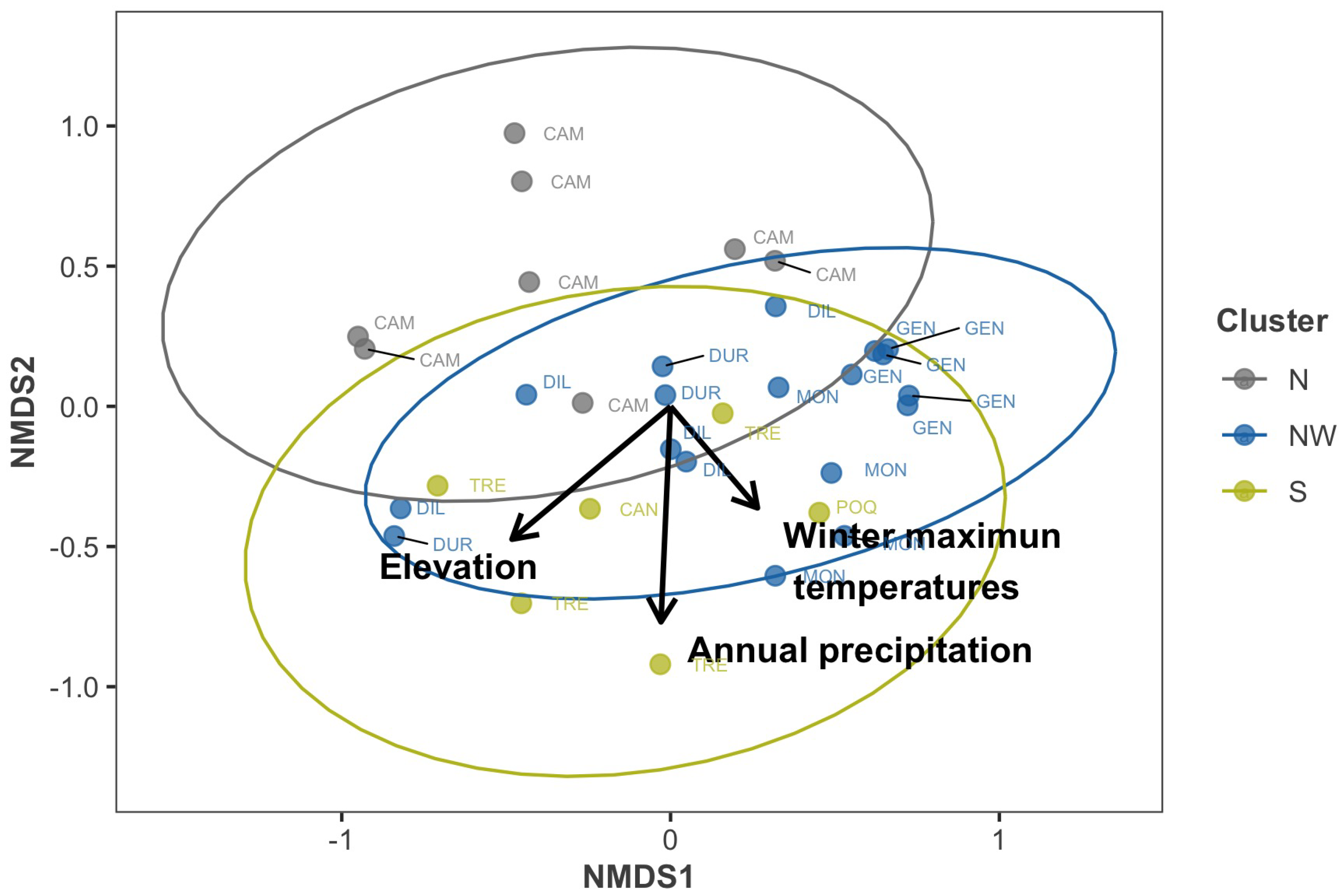
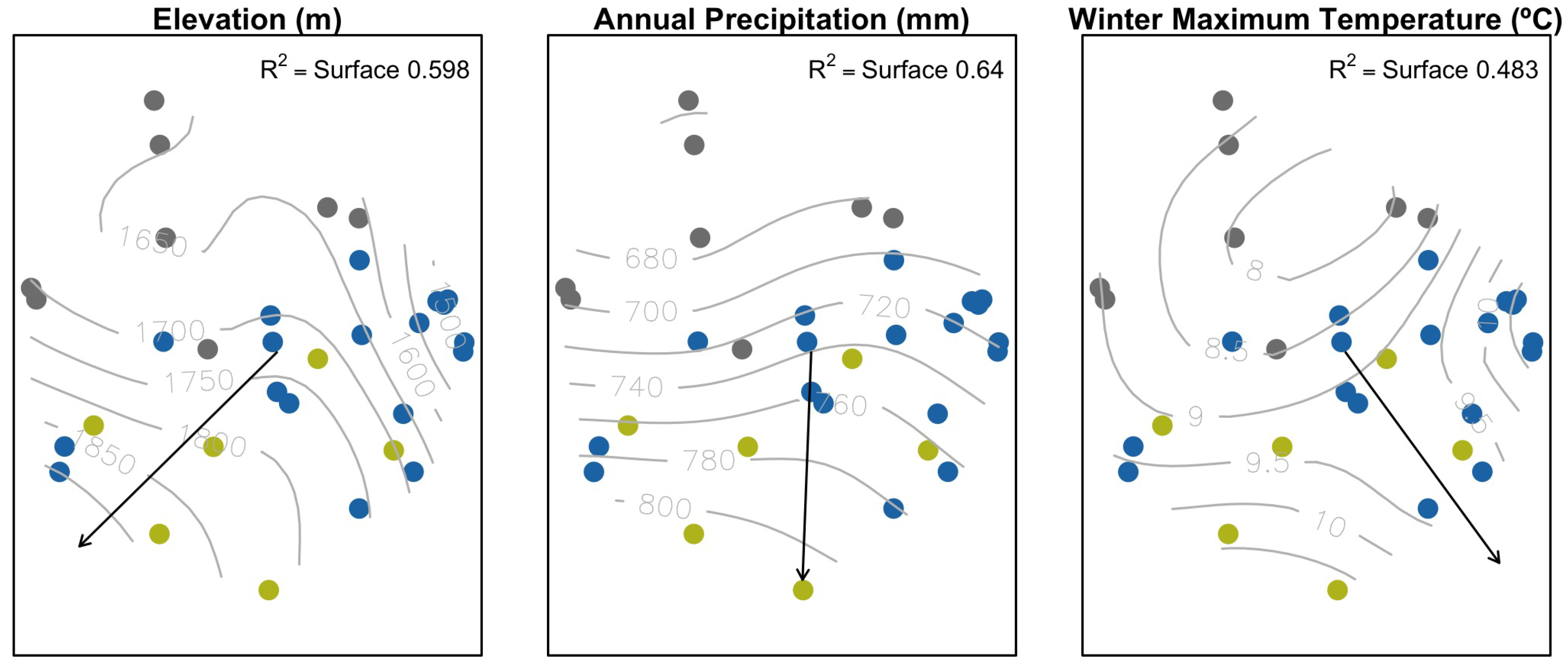
| Vector | Response Surface | ||||
|---|---|---|---|---|---|
| Variable | Vector | Vector p-Value | F | Response Surface | p-Value |
| Climate | |||||
| precWI | 0.583 | 0.001 | 4.89 | 0.587 | 0.000 |
| precSP | 0.509 | 0.001 | 6.23 | 0.644 | 0.000 |
| precSU | 0.584 | 0.001 | 7.76 | 0.693 | 0.000 |
| precAU | 0.526 | 0.001 | 2.93 | 0.460 | 0.000 |
| precYE | 0.613 | 0.001 | 6.14 | 0.640 | 0.000 |
| tminWI | 0.071 | 0.547 | 0.73 | 0.175 | 0.106 |
| tminSP | 0.091 | 0.436 | 0.63 | 0.155 | 0.121 |
| tminSU | 0.138 | 0.223 | 0.51 | 0.130 | 0.140 |
| tminAU | 0.101 | 0.384 | 0.54 | 0.137 | 0.144 |
| tmaxWI | 0.234 | 0.047 | 3.21 | 0.483 | 0.001 |
| tmaxSP | 0.112 | 0.363 | 0.87 | 0.202 | 0.069 |
| tmaxSU | 0.206 | 0.081 | 1.78 | 0.341 | 0.014 |
| tmaxAU | 0.225 | 0.057 | 2.97 | 0.463 | 0.002 |
| Landscape | |||||
| human | 0.127 | 0.277 | 0.14 | 0.040 | 0.319 |
| Topography | |||||
| twi | 0.057 | 0.649 | 0.52 | 0.131 | 0.133 |
| flow | 0.032 | 0.830 | 0.00 | 0.000 | 0.604 |
| elev | 0.464 | 0.002 | 5.12 | 0.598 | 0.000 |
| slope | 0.053 | 0.631 | 0.14 | 0.040 | 0.293 |
| tpos | 0.131 | 0.261 | 0.27 | 0.072 | 0.232 |
| aspect | 0.050 | 0.696 | 0.00 | 0.000 | 0.646 |
| tpEW | 0.050 | 0.698 | 0.34 | 0.090 | 0.217 |
| tpNS | 0.008 | 0.970 | 0.31 | 0.081 | 0.211 |
| radWI | 0.021 | 0.899 | 0.12 | 0.034 | 0.326 |
| radSU | 0.017 | 0.918 | 0.00 | 0.000 | 0.841 |
| radSP | 0.024 | 0.864 | 0.00 | 0.000 | 0.580 |
| radAU | 0.014 | 0.937 | 0.00 | 0.000 | 0.660 |
| radhWI | 0.028 | 0.837 | 0.05 | 0.014 | 0.384 |
| radhSP | 0.038 | 0.782 | 0.00 | 0.000 | 0.613 |
| radhSU | 0.139 | 0.190 | 0.01 | 0.004 | 0.421 |
| radhAU | 0.115 | 0.280 | 0.19 | 0.052 | 0.274 |
Publisher’s Note: MDPI stays neutral with regard to jurisdictional claims in published maps and institutional affiliations. |
© 2020 by the authors. Licensee MDPI, Basel, Switzerland. This article is an open access article distributed under the terms and conditions of the Creative Commons Attribution (CC BY) license (http://creativecommons.org/licenses/by/4.0/).
Share and Cite
Pérez-Luque, A.J.; Benito, B.M.; Bonet-García, F.J.; Zamora, R. Ecological Diversity within Rear-Edge: A Case Study from Mediterranean Quercus pyrenaica Willd. Forests 2021, 12, 10. https://doi.org/10.3390/f12010010
Pérez-Luque AJ, Benito BM, Bonet-García FJ, Zamora R. Ecological Diversity within Rear-Edge: A Case Study from Mediterranean Quercus pyrenaica Willd. Forests. 2021; 12(1):10. https://doi.org/10.3390/f12010010
Chicago/Turabian StylePérez-Luque, Antonio J., Blas M. Benito, Francisco J. Bonet-García, and Regino Zamora. 2021. "Ecological Diversity within Rear-Edge: A Case Study from Mediterranean Quercus pyrenaica Willd." Forests 12, no. 1: 10. https://doi.org/10.3390/f12010010
APA StylePérez-Luque, A. J., Benito, B. M., Bonet-García, F. J., & Zamora, R. (2021). Ecological Diversity within Rear-Edge: A Case Study from Mediterranean Quercus pyrenaica Willd. Forests, 12(1), 10. https://doi.org/10.3390/f12010010