Detection of Standing Deadwood from Aerial Imagery Products: Two Methods for Addressing the Bare Ground Misclassification Issue

Abstract

Deadwood mapping is of high relevance for studies on forest biodiversity, forest disturbance, and dynamics. As deadwood predominantly occurs in forests characterized by a high structural complexity and rugged terrain, the use of remote sensing offers numerous advantages over terrestrial inventory. However, deadwood misclassifications can occur in the presence of bare ground, displaying a similar spectral signature. In this study, we tested the potential to detect standing deadwood (h > 5 m) using orthophotos (0.5 m resolution) and digital surface models (DSM) (1 m resolution), both derived from stereo aerial image matching (0.2 m resolution and 60%/30% overlap (end/side lap)). Models were calibrated in a 600 ha mountain forest area that was rich in deadwood in various stages of decay. We employed random forest (RF) classification, followed by two approaches for addressing the deadwood-bare ground misclassification issue: (1) post-processing, with a mean neighborhood filter for “deadwood”-pixels and filtering out isolated pixels and (2) a “deadwood-uncertainty” filter, quantifying the probability of a “deadwood”-pixel to be correctly classified as a function of the environmental and spectral conditions in its neighborhood. RF model validation based on data partitioning delivered high user’s (UA) and producer’s (PA) accuracies (both > 0.9). Independent validation, however, revealed a high commission error for deadwood, mainly in areas with bare ground (UA = 0.60, PA = 0.87). Post-processing (1) and the application of the uncertainty filter (2) improved the distinction between deadwood and bare ground and led to a more balanced relation between UA and PA (UA of 0.69 and 0.74, PA of 0.79 and 0.80, under (1) and (2), respectively). Deadwood-pixels showed 90% location agreement with manually delineated reference to deadwood objects. With both alternative solutions, deadwood mapping achieved reliable results and the highest accuracies were obtained with deadwood-uncertainty filter. Since the information on surface heights was crucial for correct classification, enhancing DSM quality could substantially improve the results.

1. Introduction

Deadwood is an important resource for more than 30% of all forest species and thus of great relevance for forest biodiversity [1,2,3,4]. Whether standing or laying, fresh or in later stages of decay, deadwood offers a variety of microhabitats for various species [5,6,7,8], in addition to providing substrate for lichens, mosses, and fungi [9,10,11], and nutrients for a new generation of trees. Effective biodiversity conservation in forest landscapes requires information about the amount and distribution of deadwood at relevant spatial scales [12,13,14].

Mapping deadwood across large areas is therefore of general interest for biodiversity studies and nature conservation [15], although the requirements regarding the detail of deadwood mapping may vary. When assessing habitat quality for generalist species, a rough approximation of deadwood amounts may be a sufficient proxy. For specialists, a differentiation between standing and lying deadwood in various stages of decay, or even between different tree species, may be required [16,17]. In this context, remote sensing offers numerous advantages for deadwood detection, such as continuous spatial information, well-established visual interpretation keys [18,19], and automated and standardized detection methods [20,21].

Detection of deadwood from remote sensing data relies on spectral properties in the near-infrared region (NIR) of the light spectrum, reflecting the difference between vital and non-vital vegetation tissues [22], e.g., in desiccating leaves or dying trees [23,24]. Moreover, the red edge gradient between red and infrared bands and in some cases bands from the short-wave-infrared region (SWIR) [25,26] can improve the detection of deadwood in an automated process (both are not included in the standard 4 channel (red, green, blue, and near-infrared, RGBI)). To diminish the influences and interdependencies between bands, spectral indices based on algebraic combinations of reflectance in different bands were found to be helpful in mapping different land cover and object classes [27] among which is also the live, senescing, and dead vegetation [28,29].

Over decades, deadwood has been mapped visually based on color-infrared (CIR) aerial imagery and applied in forest research and management, e.g., for mapping bark beetles’ infestations [20,30,31], in forest tree health assessment [32], or in studies of forest dynamics [33] and forest wildlife ecology [34,35]. Nowadays, with the growing availability of digital optical data with very high resolutions (e.g., < 0.1 m from unmanned aerial vehicles (UAV), 0.1–0.2 m from aerial imagery and < 10 m from satellite imagery [36]) together with the availability of airborne laser scanning (ALS) data and the development of classification workflows, automated deadwood detection became possible. This brings deadwood mapping to a higher level of detail and allows standardized processing of big datasets [21].

The suitability of remote sensing data for deadwood mapping differs. The spectral information from the infrared band of aerial or satellite imagery is indispensable to detect differences between healthy, weakened, and dead vegetation. It can be used as the only input to differentiate in an analog (visual) or automated way between dead and living vegetation. The results differ depending on the study and the validation method, with overall accuracies (OA) between 0.67 and 0.94 [34,37].

To enhance deadwood detection structural information on canopy heights is helpful. For automated analyses, ALS data in combination with CIR aerial imagery showed the best results to date with OA of about 0.90 [38,39,40]. Detection of standing deadwood from ALS data was also tested and it delivered heterogeneous results, depending on forest type and detection method [41,42], with OAs from 0.65–0.73 [43,44,45] to 0.86–0.92 [35,46].

In Germany, as in many other countries, up-to-date, area-wide ALS data is rarely available, whereas CIR aerial imagery is regularly updated by state surveys. As deadwood frequently occurs in rough terrain and forest stands with high structural complexity, the use of aerial imagery data imposes challenges on deadwood detection that needs special addressing. Solar angle and viewing geometry of aerial images cause shadow occurrence and limited insight into canopy openings. These factors influence the derivation of correct canopy surface heights by image matching, especially in forest gaps and clearances or at the edges of forest roads [47,48,49]. These inaccuracies result in image and object distortions of derived “true-orthophotos”.

This is where the correct separation of dead or senescing trees from bare ground becomes challenging [25,50]. Bare ground, visible by eye through the canopy of open stands or at the border to forest roads, mimics the spectral signature of deadwood objects and is a source of misclassification in automated methods when vegetation heights are not reliable. This issue becomes particularly severe in areas where deadwood accumulates and increases stand structure complexity, e.g., after natural disturbances or in unmanaged forest reserves. Studying deadwood dynamics in these areas is particularly important for understanding natural forest development under climate change and the associated biotic and abiotic impacts on forests.

The objective of this study was to identify standing deadwood and distinguish it from live and declining trees, as well as bare ground in a semi-automatic workflow. We developed an automated procedure based on RGBI stereo aerial imagery. Random forest (RF) models were complemented with two novel approaches for addressing the “deadwood” and “bare ground” misclassification issue: (1) a post-processing procedure based on morphological analyses of RF results and (2) the application of a “deadwood-uncertainty” filter, based on a linear regression model. As input data, vegetation heights from a canopy height model (CHM) derived from a digital surface model (DSM) from image matching of aerial images, and an ALS-based Digital Terrain Model (DTM) were used. The same aerial images and DSM were used to calculate a “true-orthophoto” (termed hereafter as “orthophoto”) from which spectral variables were generated. Based on the results we evaluated the suitability of regularly updated aerial imagery data of state surveys and the products thereof as a sole basis for reliable standing deadwood detection.

2. Materials and Methods

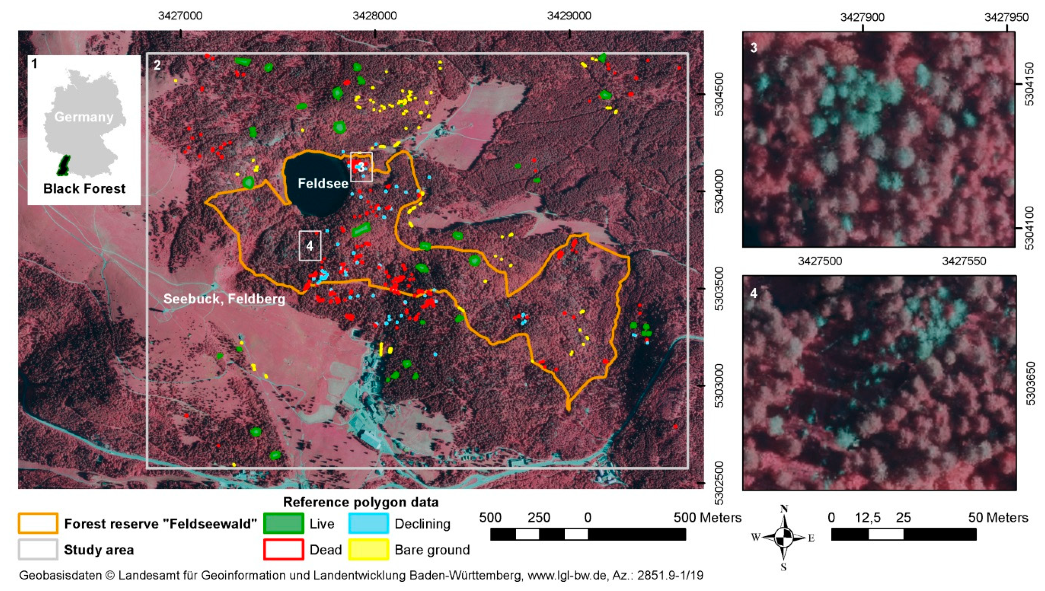
2.1. Study Site

The study area of 600 ha is located on the northern slopes of Feldberg (1493 m a.s.l.), the highest mountain in the Black Forest mountain chain (Southwestern Germany). It encompasses 102 ha of a strictly protected forest reserve, “Feldseewald”, named from the mountain glacier lake “Feldsee” located at 1100 m a.s.l. within the reserve. The terrain of the study area is characterized by steep slopes with rock formations in the northwest of the lake and smoothly rising elevations from the lake to the east and northeast (Figure 1). The temperate climate [51] is characterized by an average annual temperature of T = 3.9 °C. On average, it has 151 frost (T min < 0°C) and 75 ice days (T max < 0 °C) per year, and an average annual precipitation of 1650.0 mm [52].

The reserve is surrounded by large, managed forest stands and mountain meadows. The dominating tree species of the montane and subalpine conifer and mixed forests is Norway spruce (Picea abies) accompanied by Silver fir (Abies alba) and European beech (Fagus sylvatica). There is no intervention policy since the creation of the forest nature reserve in 1993. Natural disturbances and tree mortality are mainly caused by European spruce bark beetle (Ips typographus L.) infestations, which lead to a high abundance of deadwood in different forms and decay stages, thus making the area a suitable model region for developing and evaluating a deadwood detection method under difficult topographic conditions.

2.2. Remote Sensing and GIS Data

As primary input, we used four channels (red, green, blue, and near-infrared (RGBI)) of stereo aerial imagery with a ground resolution of 0.2 m and overlap of 60%/30% (end/side lap) owned by the State Agency of Spatial Information and Rural Development (Landesamt für Geoinformation und Landentwicklung Baden-Württemberg (LGL)) [53]. The aerial imagery was acquired on 08 August 2016 between 07:12:08–07:41:37 by airplane mission with a UC-SXp-1-30019136 camera with a focal length of 100.5 mm. Focusing on standard aerial imagery from state mapping agencies, we used aerial imagery data without radiometric enhancement. Orthophotos (0.5 m resolution) and a DSM and CHM (1 m resolution) from the LGL [53] were used to deliver both spectral and surface height information for the modelling. DSM and CHM were derived by image matching from the stereo aerial imagery using the photogrammetric software SURE [54] in line with the methodology described in Schumacher et al. [55]. The former represented the absolute top surface heights above sea level (a.s.l.) and the latter exclusively depicted the vegetation heights after subtracting DTM terrain elevation.

To avoid misclassifications with non-forest areas, only land declared as “forest” (according to the forest-ownership Geographical Information System (GIS)-layer administrated by the Department of Forest Geoinformation of Baden-Württemberg [56]) was analyzed. Standing water was masked out based on a topographical GIS-layer produced by the State Authority Topographical and Cartographical Information System (ATKIS) [57]. A DTM of 1 m resolution (LGL) [53] was used to derive slope for identifying steep rocks.

Shadow pixels were excluded from the classification to guarantee that only spectral information from the sunlit tree crowns was used. We generated two shadow masks based on hue (H) and value (V) from a hue, saturation, and value (HSV)-transformation of the RGB bands and their histograms (calculated using the package “grDevices” implemented in the software R [58]). Deep (darkest) shadow pixels (H ≥ 0.51 or V ≤ 0.18) were removed during the data preparation. Partial shadow cells (H ≥ 0.37 or V ≤ 0.24) were used later in the post-processing.

All analyses were carried out on data in raster format with 0.5 m resolution to make the best possible use of high-resolution information in the data. Data with coarser resolution were disaggregated to 0.5 m and polygon features were rasterized based on the high spatial resolution of the orthophoto and analyzed using the “raster” package in R [59]. For polygon operations the “rgdal” [60] package in R was used.

2.3. Standing Deadwood Definition and Model Classes

The aim of our study was to detect standing deadwood in different stages of decay, i.e., from recently dead trees with crown and needles to high snags (stages 3 to 6, according to Thomas et al. [61], Figure 2).

To exclude low stumps and avoid misclassifications with visible bare ground or lying deadwood, only pixels of 5 m or above in height according to the CHM were selected for the analysis. Considering the advantages of the infrared band in depicting differences in cell structure and water content in the vegetation, we did not only distinguish between “dead” and “live” (vital) vegetation but considered “declining” trees with signs of dieback, breakage, or foliage discoloration. A fourth class, “bare ground”, was included in the model to account for pixels where the CHM was not accurate enough to exclude bare ground areas.

2.4. Reference Polygons for Model Calibration

In total, 515 reference polygons were digitized as reference data pool for model training, as well as for the validation on pure classes and a polygon-based validation (

Table 1. Reference polygons, their number/size per class, and the amount of pixels available for training and validation on “pure classes” after converting polygon areas into raster maps with 0.5 m resolution.

Model Class	N	Polygon Area (m2)						No. of Pixels
		Sum	Min	Max	Mean	Median	SD
live	33	24,789.7	1.2	2797	751.2	576.6	659.9	98,137
dead	315	4295.7	0.1	65.9	13.6	11	12.1	17,143
declining	64	1510.8	6.9	52.0	23.6	22.1	10.7	6048
bare ground	103	1208.9	0.5	178.7	11.7	4.2	22.3	4272

). The reference data was collected mainly from the forest reserve and adjacent stands, where selected trees of the classes “dead” and “declining” had been additionally verified in the field in 2017.

The reference polygons of the classes “dead” and “declining” were delineated as single tree objects, while “bare ground” and the “live” stand was mostly mapped as larger uniform areas to include potential partial shadows between trees standing close to each other. While delineating the reference data we made sure to create uniform object classes, while at the same time including the variability within the classes, e.g., selecting deadwood of various sizes and stages of decay. The objects were also chosen from diverse spatial locations of the study area to account for regional differences and Bidirectional Reflection Distribution Function (BRDF) effects [62].

The collected polygon data was rasterized with each pixel having its center inside the polygon assigned to the respective class.

The polygon sizes for the class “dead” varied from 0.1 (snags) to 65.9 m² (with a median of 11 m² (corresponding to a dead tree with branches of 1.5–2.0 m length) (Table 1). Declining trees had larger crowns and a minimum polygon size of 6.9 m² (median: 22.1 m²).

2.5. Deadwood Detection Method

The deadwood detection method was developed in the analysis steps, as depicted in Figure 3. First, a RF model (“DDLG”) was calibrated for predicting the model classes: “dead”, “declining”, “live”, and “bare ground”. The following two scenarios aimed at improving the differentiation between deadwood and bare ground: Firstly, a post-processing procedure (DDLG_P), estimating the probability of “deadwood”-pixel with a mean neighborhood filter and removing isolated pixels causing the so called “salt and pepper”-effect [63]; Secondly, the application of a deadwood-uncertainty filter for identifying unreliable deadwood patches (DDLG_U).

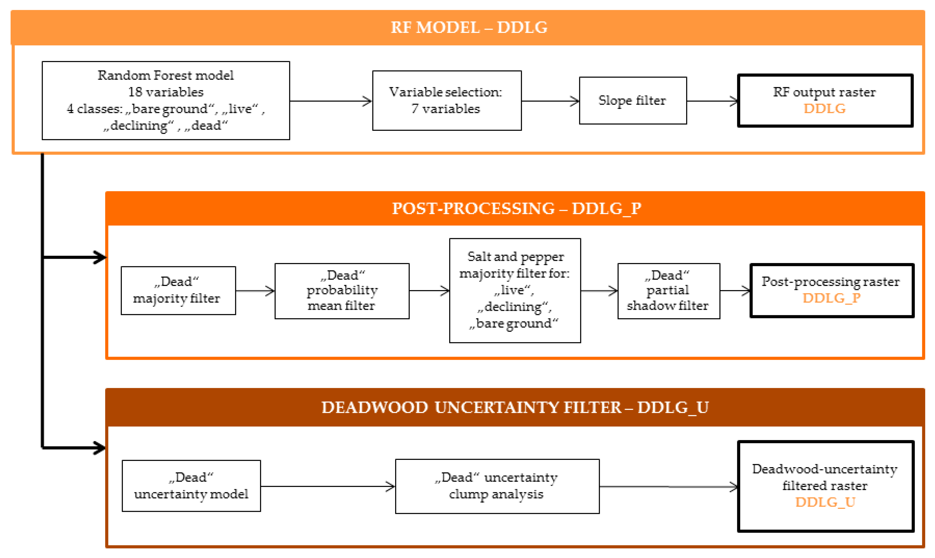
2.5.1. Random Forest Model (DDLG)

The RF algorithm [64] implemented in the R-package “caret” [65] was used in the first step (DDLG) as a classifier to distinguish standing deadwood from the three other model classes. We trained the RF model (DDLG) using 2000 pixels per class, randomly drawn from the reference polygons.

The model was run 15 times using 3 repetitions and 5-fold cross-validation with 10 variables at each split, allowing 500 trees. Model input consisted of 18 variables: red (R), green (G), blue (B), and infrared (I) spectral bands of the orthophoto and ratios thereof (

Table 2. List of ratios tested as predictor variables for the random forest (RF) model. Variables selected in the final model are displayed in bold.

Predictor Variables	Description or Formula	Reference
R, G, B, I	Red, green, blue, infrared bands	-
H, S, V	Hue, saturation, value calculated with “rgb2hsv” function in “grDevices”	R-package “grDevices” [58]
Vegetation_h	Vegetation height from CHM	-
R_ratio	R/(R + G + B + I)	Ganz [66]
G_ratio	G/(R + G + B + I)
B_ratio	B/(R + G + B + I)
I_ratio	I/(R + G + B +I)
NDVI	(I − R)/(I + R)	Jackson and Huete [67]
NDVI_green	(I − G)/(I + G)	Ahamed et al. [68]
G_R_ratio	G/R	Waser et al. [28]
G_R_ratio_2	(G − R)/(G + R)	Gitelson et al. [69]
B_ratio_2	(R/B) × (G/B) × (I/B)	self-developed after Waser et al. [28]
B_I_ratio	B/I	self-developed

) complemented with hue, saturation, and value (HSV) and information on vegetation height (CHM). We expected the latter to improve the differentiation between standing deadwood of 5 m and more in height and bare ground with expected heights close to 0 m.

To reduce model complexity, we selected the following uncorrelated (Spearman’s r ≤ |0.7|) variables with the highest model contribution: Vegetation height (Vegetation_h), red-to-all band ratio (R_ratio), blue-to-infrared ratio (B_I_ratio), hue (H), and saturation (S). As RF algorithm can deal with correlated variables, we also included the normalized difference vegetation index (NDVI), which was correlated with R_ratio and B_I_ratio, but is a standard variable used for studies on vegetation health and deadwood detection, and the information of the blue spectral band (B) for potentially improving bare ground recognition. The contributions of the individual variables to the full and the reduced RF model are shown in

Table A1. Confusion matrix presenting the pure class validation results (confusion matrix, user’s and producer’s accuracy (in bold) and overall accuracy (in bold/italics)) of the RF model (DDLG) with (1) 18 variables versus (2) 7 variables.

DDLG			Reference				Predicted Total	User’s Accuracy
			Bare Ground	Live	Declining	Dead
18 variables	Predicted	Bare ground	1971	1	8	14	1994	0.99
		Live	1	1940	112	4	2057	0.94
		Declining	10	59	1792	145	2006	0.89
		Dead	18	0	88	1837	1943	0.95
	Reference total		2000	2000	2000	1986	7540
	Producer’s and overall accuracy		0.99	0.97	0.90	0.92		0.94
7 variables	Predicted	Bare ground	1989	0	12	22	2023	0.98
		Live	0	1930	104	4	2038	0.95
		Declining	4	66	1812	131	2013	0.90
		Dead	7	4	72	1843	1926	0.96
	Reference total		2000	2000	2000	2000	7574
	Producer’s and overall accuracy		0.99	0.97	0.91	0.92		0.95

.

Finally, to identify steep rocks and reclassify them to “bare ground”, a slope-mask was used. Derived from the DTM and smoothed using the Gaussian filter in a 3-pixel neighborhood, it was applied to the model outcome to reclassify “dead”-pixels to “bare ground” in areas with slopes > 50° and CHM-values < 15 m.

2.5.2. Post-Processing of RF Results (DDLG_P)

To enhance the results of the RF classification (DDLG), a post-processing procedure was developed to remove the salt and pepper effects (single pixels and groups of two) and to improve the differentiation between the classes “bare ground” and “dead” (Figure 3).

First, clumps of isolated deadwood pixels were identified (using the function “clump” of the “raster” package) and the amount of pixels in each clump (“dead” patch) was calculated. Clumps smaller than 0.5 m² (2 pixels) were considered unreliable and reclassified based on the most frequent pixel value occurring in its 3 × 3 pixel neighborhood (majority filter). In case isolated “dead” pixels were surrounded by no data (NA) values, they were reclassified to NA.

Hypothesizing that isolated deadwood pixels surrounded by pixels of the classes “dead” or “declining” had a higher probability to be correctly classified than when surrounded by “bare ground” or ”live”-pixels, focal statistics was applied to categorize deadwood pixels based on their surroundings. For this purpose, pixels of all classes were reclassified into: “NA” = 0, “bare ground” = 1, “live” = 2, “declining” = 3, and “dead” = 4. For each pixel, the mean value k of the neighboring pixels within a 3 × 3 pixel window was calculated. Pixels of the classes “dead” and “bare ground” with k ≥ 3.1 were classified as “dead”. The remaining “dead”-pixels were reclassified as follows: “declining” with 2.8 ≤ k < 3.1, “live” with 1.4 ≤ k < 2.8, and “bare ground” with k < 1.4.

The majority-filter to remove the salt and pepper effect was then applied a second time, this time to three remaining pixel classes. Finally, a “partial shadow-filter” was applied. Clumps of deadwood pixels located entirely (>99% of the clump size area) in partial shadow (for details see data Section 2.2) were reclassified to “bare ground”.

The steps of the post-processing procedure were calculated using packages: “raster”, “igraph” [70], and “data.table” [71] in R. The package “tictoc” [72] was applied to monitor the processing time. The results were saved as geoTiff in unsigned integer raster format.

2.5.3. Deadwood Uncertainty Filter (DDLG_U)

As an alternative solution to improve the differentiation between “bare ground” and deadwood a deadwood-uncertainty filter was developed, based on a binomial generalized linear model (GLM) that quantified the probability of a “dead”-pixel to be correctly classified (1 = “dead”, 0 = “not dead”), as a function of the surrounding environmental and spectral conditions.

To generate the training and evaluation data for this model, a visual evaluation of the results of the deadwood model layer (DDLG) was carried out. All “dead” DDLG pixels were clumped into patches (3482) and converted to polygons in ArcGIS. A random selection of 2000 clumps was visually classified into “dead” (correctly classified = 1) or “not-dead” (misclassified = 0). Where no reliable classification was possible by visual interpretation, the respective polygon was dropped. Of the 762 verified and 1236 falsified deadwood patches consisting of 23,119 and 5169 pixels, respectively, 1000 pixels per class were then randomly selected for the training and four evaluation datasets, respectively (i.e., consisting of 2000 pixels each).

Six predictor variables were entered in this model (

Table 3. Predictor variables tested for the deadwood-uncertainty model with their description, hypothesized meaning and unit. Variables selected for the final model are presented in bold. I: infrared spectral band.

Variable	Description	Hypothesized Meaning	Unit
Clump_size	Size of the “dead” pixel clumps grouped with 8 neighbors (1 pixel = 0.25 m2)	Very small and very big clumps are more likely to be falsely classified	N
Bare_ground	Proportion of bare ground within a 11.5 × 11.5 m (23 × 23 pixels) moving window	Occurrence of “bare ground” next to “dead” pixels may indicate a possible misclassification of both classes	0–1
Canopy_cover	Proportion of pixels above 2 m vegetation height within a 11.5 × 11.5 m (23 × 23 pixels) moving window	Pixels with low canopy cover are likely to have false height values in transition areas between high and low vegetation	0–1
Curvature	Curvature values per pixel based on the I band	Form and direction of the I spectral signal may differ between “dead” and “bare ground” objects	Value (−∞)–∞
Curvature_Mean	Mean curvature values within a 2.5 × 2.5 m (5 × 5 pixels) moving window based on the I band	Form and direction of the I spectral signal in a wider surrounding may show differences between “dead” and “bare ground” objects	Value (−∞)–∞
Mean Euclidean distance (texture features)	Mean Euclidean distance values within a 2.5 × 2.5 m (5 × 5 pixels) moving window based on the I band	“Dead” and “bare ground” objects may show different texture characteristics in the I band	Value 0–∞

): the clump size of the deadwood pixel, bare-ground occurrence, and canopy cover within a 11.5 × 11.5 m (23 × 23 pixels) moving window that corresponded roughly to a size of a dead tree’s crown, as well as three image texture variables, i.e., the curvature, mean value of curvature, and the mean Euclidean distance, the last two of which were calculated in a 5 × 5 pixel moving window. The last three variables were included to explore texture patterns of smaller sections of deadwood objects associated with reflection changes between single pixels and pixels regions in the infrared (I) band, e.g., at the outer parts of dead trees or in sharp borders and smooth transition areas between object classes. Curvature, describing the shape of the slope (concave, convex, or linear), here between the neighboring I-values of the aerial imagery, was calculated using “Curvature” function of ArcMap [73]. The Mean Euclidean distance between endpoints of the grey-level vector referring to window’s center pixel and the vectors of all other pixels within the moving window [74] was measured using I band as implemented in ERDAS Imagine [75].

We followed a hierarchical variable selection procedure: First, variables were tested univariately and in their quadratic form. Uncorrelated (Spearman’s r ≤ |0.7|) variables significantly contributed to correctly distinguishing falsely classified “dead” pixels (

Table A2. Variables tested and retained (in bold) in the “deadwood-uncertainty model”, a generalized linear model GLM predicting the probability of standing deadwood being correctly classified. Variables are presented with their mean and standard deviation (SD) for correctly (PRES) and falsely (ABS) classified deadwood pixels. Also provided are the p-value and AIC of univariate models including the linear (l) and quadratic (q) term of the variable. Variable codes and descriptions are listed in Table 3.

	PRES_Mean	PRES_SD	ABS_Mean	ABS_SD	p_l	AIC_l	p_q	AIC_q
Clump_size	634.17	1121.12	27.81	33.21	0.00	1791.67	0.00	1792.66
Bare_ground	0.01	0.02	0.02	0.06	0.00	2680.88	0.01	2678.66
Canopy_cover	0.97	0.08	0.91	0.13	0.00	2633.00	0.00	2601.77
Curvature	504,964.40	5,138,583.17	−510,916.80	6,535,890.74	0.00	2761.7	NA	NA
Curvature_mean	101,697.81	546,521.45	−169,517.63	520,512.28	0.00	2650.9	NA	NA
Mean_Eucklidean_ Distance	4945.16	2088.62	5078.54	3115.96	0.26	2775.3	NA	NA

). We then tested all possible combinations of these variables using the dredge-function (R-package MuMIN [76]) to select the best model based on Akaike’s information criterion (AIC). Model fit was measured by means of several evaluation metrics: the area under the receiver operating characteristics curve (AUC) as implemented in R package “AUC” [77], as well as sensitivity, specificity, positive prediction value (PPV), negative prediction value (NPV), overall accuracy (OA), and Cohen’s Kappa, as implemented in the R package “caret” and described by Hosmer and Lemeshow [78].

In addition, the uncertainty model was evaluated using four independent evaluation datasets (2000 pixels each), drawn without replacement and with an equal proportion of presence and absence observations in each set.

To analyze the influence of the single predictor variables, we plotted them against the target variable using the R-package “ggplot2” [79].

Finally, to convert continuous values into a binary filter (deadwood-classification correct/false), different cut-off values were tested: The value at Kappa maximum and the value resulting in a maximum sensitivity with a specificity of at least 0.70 (identified using the multiple optimal cut point selection with increments of 0.05, R-package “cutpointr” [80]), with the intention of keeping as many of the correctly classified “dead” pixels as possible while removing a large proportion of the falsely classified pixels.

2.6. Model Validation

2.6.1. Visual Assessment

As a first step, the outcome of all models was visually examined based on orthophoto, CHM, and stereo aerial imagery using GIS (2D) and Summit Evolution (3D) [81] to appraise the plausibility of the predictions in a real-world situation.

2.6.2. “Pure Classes” Validation

We evaluated the RF model (DDLG) using the validation dataset consisting of 2000 pixels per class, randomly drawn from the reference polygons.

The confusion matrix and associated accuracy measures, i.e., overall accuracy (OA, expressing the partition of correctly classified samples in all classes) with a 95% confidence interval (95% CI), producer’s accuracy (PA, referring to the probability that a certain class on the ground is classified as such) and user’s accuracy (UA, referring to the probability that a pixel of a given class in the map really is this class) [82], as well as Cohen´s Kappa (reflecting the overall reliability of the map [83]) were calculated for each class as implemented in the R-package “caret”, comparing each class factor level to the remaining levels (i.e., a “one versus all” approach).

2.6.3. Pixel-Based Validation Based on a Stratified Random Sample

In addition to the validation on “pure classes”, an independent stratified random sample was collected. For this purpose, 750 pixels per class (“dead”, “declining”, “live”, and “bare-ground”) with only 1 pixel randomly sampled per clump (defined based on the DDLG_P layer) were selected. Pixels were then classified by visual interpretation, with pixels of different classes randomized before interpretation to avoid any interpreters’ bias. For evaluation, the results of the visual classification were compared with the results of the three model outcomes (DDLG, DDLG_P, and DDLG_U) for generating the confusion matrices and associated accuracy measures.

2.6.4. Polygon-Based Deadwood Validation

Finally, to estimate the accuracy of single tree detection of the three modelling outcomes, the results for the class “dead” were compared with the reference polygons of “dead” class. For this purpose, an intersection analysis was conducted to assess to which extent the deadwood reference polygons intersected with pixels of the deadwood class identified by each model (DDLG, DDLG_P, and DDLG_U). ”Positive detection” was assigned, when at least one deadwood pixel (single “dead” pixels often representing deadwood in decay stages 5 or 6 (Figure 2)) intersected. In addition, we compared the overall area covered by all intersecting pixels with the area of the reference polygons.

3. Results

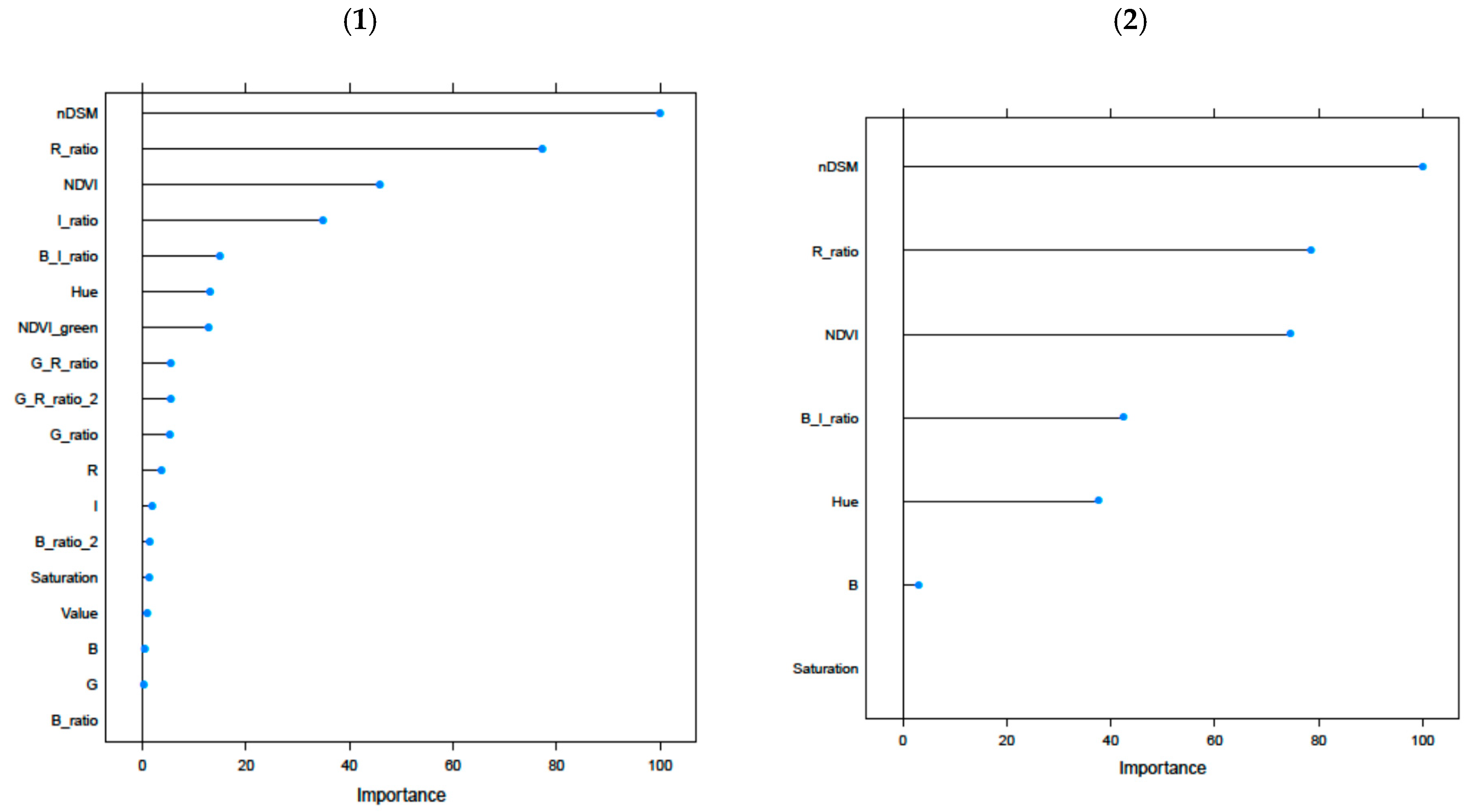
3.1. Random Forest Model and Pure Classes’ Validation

The reduced RF model based on seven variables (DDLG) performed similar compared to the initial, full model including 18 variables, with a Cohen’s Kappa of 0.92 and 0.93 and an overall accuracy of 0.95 and 0.94, respectively (

Table 4. Results of the “pure classes” validation for the DDLG model with both 18 and 7 selected variables, respectively, measured by producer’s, user’s, and overall (in bold) accuracies as well as Cohen’s Kappa. Confusion matrices are presented in (Table A1).

DDLG Version	Accuracy Measure	Class				Overall Accuracy	Kappa
		Bare Ground	Live	Declining	Dead
18 variables	Producer’s accuracy	0.99	0.97	0.90	0.92	0.94	0.93
	User’s accuracy	0.99	0.94	0.89	0.95
7 variables	Producer’s accuracy	0.99	0.97	0.91	0.92	0.95	0.92
	User’s accuracy	0.98	0.95	0.90	0.96

). All classes were predicted with very good producer’s and user’s accuracy values (all around 0.90 or above).

The most important predictor variables were vegetation height (CHM), R_ratio, NDVI, B_I_ratio, and hue (Figure A1). Vegetation heights were a key factor for separating pixels of the classes “bare ground” and “dead”. NDVI and R_ratio were especially decisive for the recognition of “live” trees, and NDVI, hue, and B_I_ratio were important for distinguishing between the classes “live”, “declining”, and “dead”. Blue band and saturation showed only little contributions to the model.

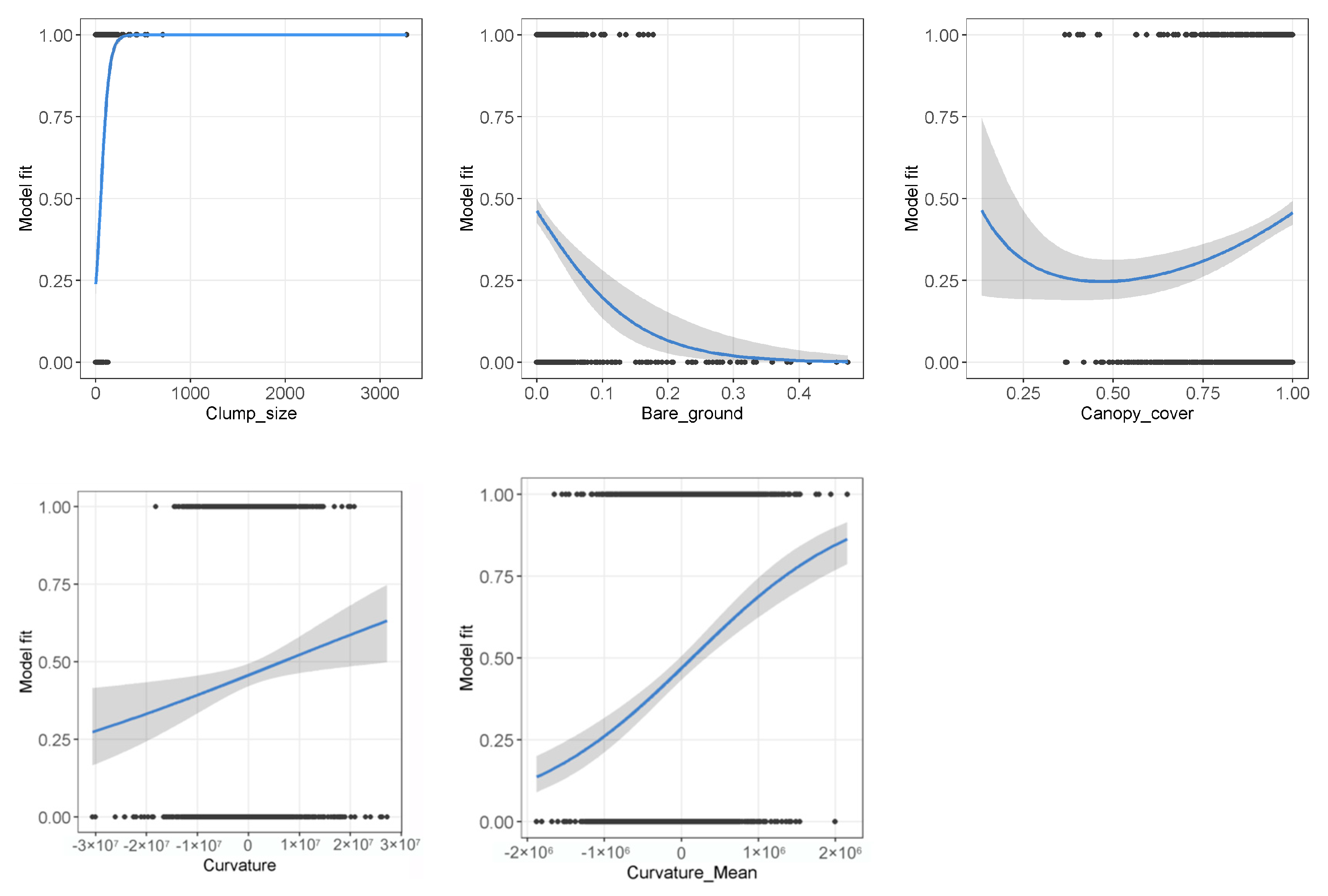
3.2. Uncertainty Model

The deadwood-uncertainty model included five of the six tested input variables (Table A2): Clump_size and Bare_ground (both as linear and quadratic terms); Canopy_cover; Curvature; and Curvature_Mean. All retained variables contributed significantly to the model. The effect plots (Figure A2) show that correct classification of deadwood was associated with larger clump sizes, higher canopy cover, and low amount of “bare ground” in the neighborhood. Moreover, deadwood was more likely to be correctly classified under higher texture parameter values (higher structural complexity).

With an AUC of 0.89, the model showed good predictive power. Cohen´s Kappa ranged between 0.58 to 0.60 and the overall accuracy between 0.79 and 0.80, depending on the selected threshold (

Table 5. Model fit and predictive performance of the “deadwood-uncertainty” model measured by sensitivity, specificity, positive prediction value (PPV), negative prediction value (NPV), overall accuracy, and Cohen´s Kappa for thresholds based on Kappa maximum (0.39) and the maximum sensitivity by the specificity of 0.70 (0.31). In addition, threshold-independent area under the ROC-curve (AUC) was provided for different classes’ separation. Independent validation was performed on four independent validation datasets with their results calculated for the selected threshold of maximum sensitivity by specificity of 0.70 (0.31). The validation results are presented below for comparison with arithmetic mean and standard error values showing the amount of variation between the results of different folds.

Performance	Model Fit		4 FOLDS Validation Max Sensitivity by Specificity = 0.70 (0.31)
metrics	Kappa maximum (0.39)	Max sensitivity by specificity = 0.70 (0.31)	Mean	Standard deviation
Sensitivity	0.82	0.88	0.89	0.007
Specificity	0.77	0.70	0.72	0.009
PPV	0.78	0.75	0.76	0.005
NPV	0.81	0.85	0.87	0.007
Overall accuracy	0.80	0.79	0.80	0.003
Cohen’s Kappa	0.60	0.58	0.61	0.005
AUC	0.89		0.90	0.005

). The Kappa maximum threshold (0.39) showed slightly better overall performance and better predictive power for identifying misclassified pixels. However, as we prioritized keeping a wrongly classified over discarding a correctly classified “dead” pixel, the maximum sensitivity by specificity of 0.70-value (0.31) was selected to discriminate between “dead” and “not-dead”.

The results of the independent model validation, using four validation folds showed consistently good model performance for all metrics (Table 5), with an average AUC-value of 0.90, mean Cohen’s Kappa of 0.61, and mean value for overall accuracy of 0.80 across folds by standard deviation of less than 0.005.

3.3. Classification Results

The different classification scenarios DDLG, DDLG_P, and DDLG_U (Table 5) resulted in different amounts of pixels per class, but showed a consistent general pattern with 39.4% “live”, 0.4%–0.5% “dead”, 5.2%–5.5% “declining”, and 0.2% “bare ground” areas. About 54.6–54.8% of the area was masked out as NA (Figure 4,

Table 6. Classification results per class in number and percent (%) of pixels (0.5 × 0.5 m) for the three classification scenarios: Random forest (RF) classification (DDLG), RF classification with post-processing (DDLG_P), and with additional deadwood-uncertainty filter (DDLG_U).

Class	DDLG		DDLG_P		DDLG_U
	Pixel	%	Pixel	%	Pixel	%
Live	9,341,179	39.4%	9,342,529	39.4%	9,341,179	39.4%
Dead	119,790	0.5%	105,661	0.4%	102,815	0.4%
Declining	1,274,349	5.4%	1,237,793	5.2%	1,274,349	5.4%
Bare ground	35,690	0.2%	36,265	0.2%	52,665	0.2%
NA	12,933,862	54.6%	12,982,622	54.8%	12,933,862	54.6%
Total	23,704,870	100.0%	23,704,870	100.0%	23,704,870	100.0%

).

With post-processing, the amount isolated pixels of the classes “dead”, “declining” and “bare ground” decreased, mostly in favor of “live” pixels (Table 6, Figure 4). The uncertainty filter targeting at a better differentiation between “dead” and “bare ground” changed the proportions of these two classes from about 3/1 to 2/1 (Table 6).

The number of deadwood clumps (“dead”-pixels consolidated to patches) (

Table 7. Classification results for deadwood patches (clumps of pixels classified “dead”) expressed in the number of pixels (size 0.5 × 0.5 m) per classification scenario: Random forest (RF) classification (DDLG), RF classification with post-processing (DDLG_P), and with “deadwood-uncertainty” filter (DDLG_U).

	DDLG		DDLG_P		DDLG_U
	Pixel	m2	Pixel	m2	Pixel	m2
N	9868		3482		3139
SUM	119,790.00	29,947.50	105,661.00	26,415.25	102,815.00	25,703.75
MEAN	12.14	3.04	30.34	7.59	32.75	8.19
MEDIAN	2.00	0.50	10.00	2.50	12.00	3.00
MIN	1.00	0.25	1.00	0.25	1.00	0.25
MAX	3281.00	820.25	3258.00	814.50	3281.00	820.25
SD	53.82	13.45	87.30	21.82	91.98	22.99

) decreased successively from almost 10,000 (DDLG) to 3482 in DDLG_P and 3139 in DDLG_U, while their total area decreased from 2.99 ha to 2.64 and 2.57 ha, respectively. In all cases, small deadwood patches dominated with a median size of 0.5 for DDLG and 2.25–3.00 m² for DDLG_P and DDLG_U, a minimum size of 0.25 m² (1 pixel) and a maximum size of over 814.50 m² (a large group of dead trees aggregated to one patch).

3.4. Model Validation

3.4.1. Visual Assessment

The visual assessment carried out parallel to the statistical validation did not confirm the high accuracy values of the pure class validation of the DDLG model. Visual control identified rocks and bare ground within the forest stands and on forest stand borders being misclassified as “dead”, not conforming to the high accuracy values for predicting this class and to the almost 100% accuracy for the class “bare ground”.

3.4.2. Pixel-Based Validation

For all three classification scenarios, validation on an independent, stratified random sample of pixels showed lower accuracies per class than that obtained with pure classes’ validation on the DDLG. Cohen’s Kappa (0.59–0.65) and overall accuracies (0.70–0.74) (

Table 8. Results of the validation on an independent stratified random sample of 750 pixels per class for the three classification scenarios: Random forest (RF) classification (DDLG), RF classification with post-processing (DDLG_P), and with deadwood-uncertainty filter (DDLG_U). Presented are producer’s, user’s, and overall accuracy, as well as Cohen’s Kappa (the last two indicated in bold). Detailed confusion matrices with the amount of validated pixels per class are shown in Table A3.

Model Scenario	Accuracy Measure	Class				Overall Accuracy	Kappa
		Bare Ground	Live	Declining	Dead
DDLG	User’s accuracy	0.82	0.77	0.67	0.60	0.70	0.60
	Producer’s accuracy	0.57	0.79	0.56	0.87
DDLG_P	User’s accuracy	0.75	0.73	0.61	0.69	0.70	0.59
	Producer’s accuracy	0.66	0.79	0.55	0.79
DDLG_U	User’s accuracy	0.76	0.77	0.66	0.74	0.74	0.65
	Producer’s accuracy	0.82	0.77	0.56	0.80

) were of similar magnitude for all three scenarios, with the best results for DDLG_U.

The greatest balance between producer’s and user’s accuracies were consistently achieved for the class “live” with PA of 0.79 for the DDLG and 0.77 for the two other scenarios and UA of 0.77 (DDLG, DDLG_U) and 0.73 (DDLG_P). The drop in PA after post-processing was probably caused by the majority filter to smooth the results. The class “live” had the most misclassifications with the class “declining”, for which classification was generally the least reliable (PA of 0.55–0.56 and UA of 0.61–0.67), and additional misclassifications occurred with the class “dead”. “Bare ground” classified by DDLG achieved PA = 0.57 and UA = 0.82 and was almost exclusively misclassified as “dead”. This improved with post-processing to PA = 0.66 and to PA = 0.82 after applying the uncertainty filter. Simultaneously, the UA dropped from 0.82 to 0.75 (DDLG_P) and 0.76 (DDLG_U).

The classification of “dead” pixels showed the best PA = 0.87 in the first scenario (DDLG). On the other hand, a low UA = 0.60 indicated a high commission error, with misclassifications especially in the classes “bare ground” (283 pixels) and “declining” (138 pixels) (

Table A3. Results of the validation of the three deadwood classification models Random Forest (RF) classification (DDLG), RF classification with post-processing (DDLG_P), and after applying a deadwood-uncertainty filter (DDLG_U) based on a stratified random sample (750 pixels per class). Results are presented as confusion matrix, user’s and producer’s accuracy are in bold and overall accuracy in bold/italics.

			Reference				Total Predicted	User’s Accuracy
			Bare Ground	Live	Declining	Dead
DDLG	Predicted	Bare ground	427	4	26	64	521	0.82
		Live	8	590	163	3	764	0.77
		Declining	32	148	423	30	633	0.67
		Dead	283	7	138	653	1081	0.60
	Total reference		750	749	750	750	2093
	Producer’s and overall accuracy		0.57	0.79	0.56	0.87		0.70
DDLG_P	Predicted	Bare ground	492	7	51	110	660	0.75
		Live	29	595	186	7	817	0.73
		Declining	71	146	410	42	669	0.61
		Dead	158	2	103	591	854	0.69
	Total reference		750	750	750	750	2088
	Producer’s and overall accuracy		0.66	0.79	0.55	0.79		0.70
DDLG_U	Predicted	Bare ground	612	8	67	119	806	0.76
		Live	3	581	167	3	754	0.77
		Declining	30	155	421	28	634	0.66
		Dead	105	6	95	600	806	0.74
	Total reference		750	750	750	750	2214
	Producer’s and overall accuracy		0.82	0.77	0.56	0.80		0.74

). Post processing and the application of the deadwood-uncertainty filter, both led to a more balanced PA to UA relationship. UA increased significantly from 0.60 (DDLG) to 0.69 (DDLG_P) and 0.74 (DDLG_U), whereas PA decreased from 0.87 to 0.79 and 0.80 for the same scenarios.

3.4.3. Polygon Based Deadwood Validation

The polygon-based validation confirmed good detection of standing deadwood objects with 91%–96% of the reference deadwood-patches and 90% of their area being detected in all classification scenarios (

Table 9. Results of the polygon-based validation. Basic statistics (N, % of N reference polygons, (in bold), area sum, percent of the reference area (in bold), area mean, median, maximum, and standard deviation) for the deadwood patches identified by the three classification scenarios: Random forest (RF) classification (DDLG), RF classification with post-processing (DDLG_P), and with a deadwood-uncertainty filter (DDLG_U), that were validated (intersected) and not validated (not intersected) when compared with the reference deadwood polygons.

Polygon Data	DDLG		DDLG_P		DDLG_PU
	Intersected	Not Intersected	Intersected	Not Intersected	Intersected	Not Intersected
N	303	12	287	22	291	24
N (% of reference)	96%	4%	91%	7%	92%	8%
AREA SUM (m2)	3868.5	7.5	3844.7	23.1	3855.2	22.3
AREA (% of reference)	90%	0%	90%	1%	90%	1%
AREA MEAN (m2)	12.8	0.6	13.4	0.8	13.2	0.9
AREA MEDIAN (m2)	10.4	0.1	10.6	0.7	10.6	0.5
AREA MAX (m2)	64.9	4.3	65.1	4.3	64.9	4.3
AREA SD (m2)	11.5	1.2	11.5	0.9	11.5	1.1

). Mean (12.8–13.4) and median (10.4–10.6) patch-size, and their standard deviation (11.5), showed similar values for both the intersected and the reference polygons, indicating that detected deadwood patches correctly depicted the “real” deadwood occurrence in most cases.

The intersection of the deadwood reference polygons with the patches constructed from pixels classified as “dead” showed that their total area exceeded the total area of the reference polygons by 40% in all three classification scenarios: DDLG, DDLG_P, and DDLG_U (

Table A4. Basic statistics summary (number and area) of deadwood-patches, identified by the three classification scenarios: Random forest (RF) classification (DDLG), RF classification with post-processing (DDLG_P), and with additional deadwood-uncertainty filter (DDLG_U), compared to the visually delineated reference polygons used for validation.

	Reference Polygons	DDLG	DDLG_P	DDLG_U
N	315	323	238	285
AREA SUM (m2)	4295.7	6034.8	6024.5	6013.5
% of reference polygons	100%	145%	145%	144%
AREA MEAN (m2)	13.6	18.7	25.3	21.1
AREA MEDIAN (m2)	11.0	5.2	11.0	6.5
AREA MAX (m2)	65.9	813.8	811.0	813.8
AREA SD (m2)	12.1	56.6	64.6	59.8

). The maximum area of a single deadwood-patch of 811–813.8 m² (identified by all 3 scenarios) compared to the maximum size of a single reference polygon of 65.9 m² indicated grouping of several deadwood-objects into one patch.

For DDLG, the number of intersecting deadwood-patches (323) was larger than those of the reference polygons (315). For DDLG_P and DDLG_U the number of deadwood patches and accordingly the number of intersecting deadwood-patches dropped to 76% (238) and 90% (285) of the reference polygon numbers (Table A4). Given detection rates of more than 90% (Table 9) this again indicates clustering of pixels of several dead trees into a larger patch. The number of omitted (i.e., not detected) polygons (Table 9) was lowest for DDLG and highest for DDLG_P, with an increasing trend of omitting small polygons for DDLG_U and DDLG_P. The mean area of the not detected polygons was less than 1 m² and the median less than 0.7 m², corresponding to 1–3 pixel. The total area of omitted deadwood did not exceed 1% in either scenario.

4. Discussion

4.1. Deadwood Detection

With RF classification, we used a standard procedure to detect standing deadwood and distinguish it from living and declining trees, as well as bare ground. Although the validation on pure classes appeared promising, with very high accuracies above 0.90, visual assessment revealed grave misclassifications of “bare ground” as “deadwood”. This result was confirmed when applying an independent, random sampling validation, revealing a low UA of 0.60 (Table 8). The latter improved with post-processing (UA = 0.69) and the application of a deadwood uncertainty filter (UA = 0.74), but for the price of decreasing PA from 0.87 to 0.79 and 0.80, a reliable and satisfactory level. OA remained constant for DDLG and DDLG_P at 0.7 and increased to 0.74 for DDLG_U. This level of accuracy places our method in line with visual methods based on CIR aerial imagery and methods for detecting snags using solely ALS data, e.g., Yao et al. [44] with OA of 0.70–0.75. Combining CIR and ALS data delivered mostly better results with OA between 0.83 [84] and >0.9 [38,39] depending on the algorithm used.

The polygon-based validation, with more than 90% of the deadwood-patches and their area correctly identified, proved a very good detectability of single dead trees. Not-detected polygons with a median area of 1–3 pixels in all classification scenarios indicated the biggest problems in the detection of snags and small dead crowns. This is in line with Wing et al. [85], who showed detection reliability rising with the tree’s diameter at breast height (DBH) and Krzystek et al. [40] who found lower accuracies for snags (UA = 0.56, PA = 0.66) than for dead trees (UA and PA > 0.90). Although our method was pixel-based, the deadwood-detection accuracy corresponded with the accuracy of 0.71–0.77 (by 1 to 1 pixel correspondence) achieved by Polewski et al. [86] using object detection methods based on ALS and CIR aerial imagery.

The larger overall area of our classified deadwood patches compared to the area of the reference polygons partially resulted from aggregating pixels to coarse clumps encompassing several neighboring dead trees. However, for many ecological questions and applications in practical forestry, identifying single deadwood objects and quantifying their size is important and can give a hint, e.g., on the decay stage of a dead tree [16]. Our pixel-based method produced information on the location and area of standing deadwood together with a probability that a pixel was correctly classified. Adding object detection would thus be a valuable extension of our method.

Adamczyk and Bedkowski [23] underlined the difficulty in deadwood detection, as spectral differences between the classes are fluent and influenced by light conditions, the location of the tree, crown geometry, and individual trees coloring [23]. We decided to use declining trees as a supporting class, having in mind that especially in the outer parts of crowns there is no sharp transition between a healthy crown and bare ground or the live stand. As expected, the PAs for this class were constantly the lowest (0.55–0.56) across all scenarios, as this class was not targeted for improvement. Although not highly reliable (UA between 0.61 and 0.67) the trees identified as “declining” still have a potential to be used in forestry practice for identifying trees differing from the rest of the stand, e.g., by showing dry branches, breakage, or lichens in the crown, or being weakened and thus potentially prone to or in early stage of insect (e.g., bark beetle) infestation.

4.2. Bare Ground Issue

The class “bare ground” occurred to be the key to the optimization of our deadwood detection method. Problems with discriminating between soil and deadwood were also pointed out by Fassnacht et al. [25] and Meddens et al. [50], who observed that misclassifications occurred mostly in sunned parts of dead trees. Most studies mapping senescent or dead trees from remotely sensed data neglect the possible confusion with bare ground. The magnitude of this issue largely depends on the amount of bare ground in the study area. Forest regeneration regime and soil productivity also play a role, when areas remain non-vegetated for long times after disturbance events [25]. Given the high proportion (38%) of “bare ground” pixels misclassified as “dead” in the DDLG raster, which dropped to 21% (DDLG_P) and 14% (DDLG_U), we claim that for reliable deadwood mapping this potential error needs to be addressed, especially if the results are intended for nature conservation measures, forestry operations, or field campaigns that would incur a waste of resources if planned where no dead trees were present [87]. On the other hand, increasing “bare ground” detection on the cost of reducing PA of deadwood could be disadvantageous if the goal was to identify dead trees for traffic safety, where detection of every dead tree is important [88].

Degrading the image resolution from 0.3 to 2.4 m enabled Meddens et al. [50] resolving the “bare ground” versus “dead” misclassification problem. This underlines the necessity of using data of a resolution that matches the resolution of the analyzed objects. Hengl [89] proposed a minimum of four pixels for representing the smallest circular objects and at least two pixels for representing the narrowest objects as vital for reliably detecting an object in an image, while Dalponte et al. [90] recommended the spatial resolution of the imagery to match the expected minimum size of the tree crowns in the scene. Exploring the optimal spatial resolution of multispectral satellite images for detecting single dead trees in forest areas Pluto-Kossakowska et al. [91] found 0.5–1 m to be the best pixel size. In that respect, the 0.5 m resolution in our study seems to be a good choice when aiming at mapping all standing deadwood including single snags without branches (i.e., corresponding to one to a few pixels in size).

Resampling images of coarser resolution did not achieve good results in single tree detection. However, a pixel size of >2.5 m can be enough if the goal of the study is the detection of deadwood-patches, not single trees, as already used in some applications, e.g., for planning forest operations [38]. Quantifying the effect of degrading the resolution (e.g., to 1 × 1 m) on the classification results would be an important future research topic, as this would strongly reduce processing time and the amount of data. Still, the intended practical use of the model results will always be a critical factor for defining the appropriate method.

4.3. Canopy Height Information

As we limited our scope to the detection of standing deadwood while neglecting lying deadwood, a 5 m height mask based on the CHM was included in the model set-up at the very beginning to mask out all areas close to the ground. The same was proposed by Fassnacht et al. [25] for a better separation of forest from non-forest areas. They suggested using vegetation height information provided by the spaceborne mission TanDEM-X or stereo-photogrammetry of overlapping aerial photographs in combination with an accurate DTM from ALS data. Our results, based on the second option, show that the CHM was insufficient for detecting small forest openings with bare ground which could possibly be detected when using ALS data [48].

The accuracy of digital surface models is highly related to the point density acquired either by ALS or by the matching of overlapping aerial images, with the former achieving much higher point densities. The amount of points matched from stereo aerial imagery depends on numerous factors e.g., image resolution, overlap between neighboring images, image geometry, light, and weather conditions at the time of data acquisition [47]. In shaded areas and near the ground surface with surrounding higher vegetation matching success is limited [92,93].

The aerial imagery material we used was acquired in August in the morning (7–9 a.m.) and thus image quality was negatively affected by grave occurrence of shadow and varying spectral signals. Controlling the flight times to limit shadow occurrence, as well as increasing the resolution and overlap of the stereo imagery, would certainly enhance the quality of the orthophotos and DSMs derived from the data, and consequentially enhance the accuracy of both spectral and structural predictor variables and classification results.

Information on vegetation height was among the most important predictor variables in both our RF model and the deadwood-uncertainty model. We expect that using ALS data for deriving DSM and CHM would bear the greatest potential for model improvement. In many countries, e.g., in Scandinavia [94] or Canada [36], ALS data is already a standard element of the mapping services provided by the public authorities and widely used in forestry, as delivering accurate information on canopy heights, tree species, and timber volume for forest management.

4.4. Deadwood Detection Algorithms

In the last two decades, various machine learning (ML) algorithms have been used for image classification [95,96] in the field of forest ecology. Also in deadwood detection ML algorithms, such as maximum likelihood [88,91], RF [37], or supported vector machines (SVM) [25], were applied.

We used RF as it demands little parametrization, being at the same time robust to large datasets and not requiring a-priori assumptions on statistical distributions [97]. Even though RF can deal with correlated variables, we reduced the number of predictors from 18 to 7 variables to save processing time. The results of both models showed similarly high accuracies when validated on the pure classes’ dataset, which was our reason for focusing on improving the classification results by post-processing and extra filtering instead of further optimizing the RF model.

After vegetation height, other important variables were R_ratio, NDVI, B_I_ratio and hue, what confirms the higher suitability of ratios and indices for image classification than the use of pure bands [28,67] and that the crucial spectral information was found in red, infrared, and blue bands.

Both alternative solutions applied to enhance the RF output (DDLG) improved the classification results in the targeted classes “dead” and “bare ground”. Post-processing (DDLG_P) incorporated a mean neighborhood filter for “dead” pixels assuming a lower accuracy of dead pixels in the neighborhood of “bare ground” and a “salt and pepper effect” filter removing isolated pixels of all classes, which are considered as most prone to errors. This process enhanced the separation of the classes “dead” and “bare ground”, and the overall classification results to acceptable accuracies of UA = 0.69 by PA = 0.79.

The best results, however, were achieved when applying the deadwood uncertainty filter with UA = 0.74 and PA = 0.80 for “dead” and UA = 0.76 and PA = 0.82 for “bare ground” (DDLG_U). Texture patterns of the infrared band and structural variables (canopy cover and neighboring “bare ground” pixels) included in the deadwood-uncertainty model were crucial for separating correctly classified “dead”-pixels from misclassified ones. However, since the texture variables needed extra pre-processing and the uncertainty model itself required time for the generation of new training data and model calibration, this approach was more costly compared to post-processing.

In recent years, deep learning (DL) algorithms have become increasingly popular for analyzing remote sensing data [98]. In deadwood mapping, they showed good results for identifying windthrow areas [99] or detecting deadwood objects with high resolution CIR aerial imagery [100]. Convolutional neural networks (CNN), which use different levels of generalization of the same data [101], could possibly help to correctly delineate deadwood objects that are characterized by smooth transition edges. The variables Curvature and Curvature_mean significantly contributed to the deadwood-uncertainty model, representing different aggregation levels of the same structure and suggesting a potential benefit of using CNNs. Exploring the capability of DLAs to deal with large datasets of high resolution (0.5–1 m) for large-scale deadwood detection is thus a promising future research direction.

Our method using solely RGBI of true-orthophotos and CHM data based on the same aerial images could potentially be transferred to other areas, for which similar spectral and structural digital information is available. However, the requirements and possibilities for model transferability to areas with different quality aerial imagery and other forest types need to be evaluated. Our study was conducted using data from temperate mountain spruce and mixed forests. Coniferous trees dominating in the area are characterized by compact crown shapes what implies possible limitations in stands with higher admixture of broadleaved trees featuring more irregular crown shapes. On the other hand, the CHM heights might be more accurate and bare ground better visible in stands located in areas with more smooth or plain terrain.

The method could also be tested on VHR satellite imagery data such as WorldView-3 [102], WorldView-4 [103], or Pléiades [104], particularly with regard to large-scale applications [91,105]. More research is required on how to use satellite stereoscopic data for generating both spectral and structural information for analyses and applications in ecology. Yet, when combining spectral information from VHR satellite imagery with vegetation heights from CHMs based on other data sources, particular attention needs to be paid to proper data pre-processing including atmospheric correction, accurate georeferencing, and co-registration with the DSM and subsidiary data.

5. Conclusions

We presented two alternative methods for enhancing pixel-based standing deadwood detection based on RF classification, using either post-processing or a deadwood-uncertainty filter. Both methods proved to deliver satisfactory results in a standardized automated manner, but the best accuracies were achieved when applying the deadwood-uncertainty filter. Problems with differentiating between deadwood and bare ground at forest borders and in areas with heterogeneous vegetation heights were addressed and partially solved, leading to more balanced accuracies for “deadwood” and “bare ground” classification. In this context, we also showed the misleading results of pure-classes validation and highlight the need for various independent validation methods including visual appraisal.

Our methods were solely based on spectral variables and vegetation heights derived from RGBI spectral bands and the CHM and can potentially be used for other datasets containing this information. For further improvement we suggest using ALS as a source for reliable surface heights or stereo aerial imagery with higher resolution and overlap. The latter becoming successively more and more available could deliver DSMs and “true-orthophotos” of superior detail and accuracy. Finally, object based image analysis enabling the mapping of single dead tree polygons could be an additional step in our analysis and added value for forest ecology studies and management applications based on these data, e.g., for habitat suitability modelling, monitoring of deadwood, and forest development, or for the evaluation of deadwood enrichment programs.

References

1. Thorn, S.; Müller, J.; Leverkus, A.B. Preventing European forest diebacks. Science 2019, 365. [Google Scholar] [CrossRef]
2. Hahn, K.; Christensen, M. Dead Wood in European Forest Reserves—A reference for Forest Management. In EFI Proceedings No. 51. Monitoring and Indicators of Forest Biodiversity in Europe—From Ideas to Operationality; European Forest Institute: Joensuu, Finland, 2004; pp. 181–191. [Google Scholar]
3. Schuck, A.; Meyer, P.; Menke, N.; Lier, M.; Lindner, M. Forest biodiversity indicator: Dead wood-a proposed approach towards operationalising the MCPFE indicator. In EFI Proceedings 51. Monitoring and Indicators of Forest Biodiversity in Europe—From Ideas to Operationality; Marchetti, M., Ed.; EFI: Joensuu, Finland, 2004; pp. 49–77. [Google Scholar]
4. Paillet, Y.; Berges, L.; Hjalten, J.; Odor, P.; Avon, C.; Bernhardt-Romermann, M.; Bijlsma, R.J.; De Bruyn, L.; Fuhr, M.; Grandin, U.; et al. Biodiversity differences between managed and unmanaged forests: Meta-analysis of species richness in Europe. Conserv. Biol. 2010, 24, 101–112. [Google Scholar] [CrossRef] [PubMed]
5. Müller, J.; Bußler, H.; Bense, U.; Brustel, H.; Flechtner, G.; Fowles, A.; Kahlen, M.; Möller, G.; Mühle, H.; Schmidl, J.; et al. Urwald relict species—Saproxylic beetles indicating structural qualities and habitat tradition. Wald. Online 2005, 2, 106–113. [Google Scholar]
6. Seibold, S.; Brandl, R.; Buse, J.; Hothorn, T.; Schmidl, J.; Thorn, S.; Müller, J. Association of extinction risk of saproxylic beetles with ecological degradation of forests in Europe. Conserv. Biol. 2014, 29, 382–390. [Google Scholar] [CrossRef]
7. Pechacek, P.; Krištín, A. Comparative diets of adult and young Threetoed Woodpeckers in a European alpine forest community. J. Wildl. Manag. 2004, 68, 683–693. [Google Scholar] [CrossRef]
8. Kortmann, M.; Hurst, J.; Brinkmann, R.; Heurich, M.; Silveyra González, R.; Müller, J.; Thorn, S. Beauty and the beast: How a bat utilizes forests shaped by outbreaks of an insect pest. Anim. Conserv. 2018, 21, 21–30. [Google Scholar] [CrossRef] [Green Version]
9. Olchowik, J.; Hilszczanska, D.; Bzdyk, R.; Studnicki, M.; Malewski, T.; Borowski, Z. Effect of Deadwood on Ectomycorrhizal Colonisation of Old-Growth Oak Forests. Forests 2019, 10, 480. [Google Scholar] [CrossRef] [Green Version]
10. Baldrian, P.; Zrůstová, P.; Tláskal, V.; Davidová, A.; Merhautová, V.; Vrška, T. Fungi associated with decomposing deadwood in a natural beech-dominated forest. Fungal Ecol. 2016, 23, 109–122. [Google Scholar] [CrossRef]
11. Bader, P.; Jansson, S.; Jonsson, B.G. Wood-inhabiting fungi and substratum decline in selectively logged boreal spruce forests. Biol. Conserv. 1995, 72, 355–362. [Google Scholar] [CrossRef]
12. Stighäll, K.; Roberge, J.-M.; Andersson, K.; Angelstam, P. Usefulness of biophysical proxy data for modelling habitat of an endangered forest species: The white-backed woodpecker Dendrocopos leucotos. Scand. J. For. Res. 2011, 26, 576–585. [Google Scholar] [CrossRef]
13. Braunisch, V. Spacially Explicit Species-Habitat Models for Large-Scale Conservation Planning. Modelling Habitat Potential and Habitat Connectivity for Capercaillie (Tetrao urogallus). Ph.D. Thesis, Albert-Ludwigs-Universität, Freiburg im Breisgau, Germany, 2008. [Google Scholar]
14. Kortmann, M.; Heurich, M.; Latifi, H.; Rösner, S.; Seidl, R.; Müller, J.; Thorn, S. Forest structure following natural disturbances and early succession provides habitat for two avian flagship species, capercaillie (Tetrao urogallus) and hazel grouse (Tetrastes bonasia). Biol. Conserv. 2018, 226. [Google Scholar] [CrossRef]
15. Bouvet, A.; Paillet, Y.; Archaux, F.; Tillon, L.; Denis, P.; Gilg, O.; Gosselin, F. Effects of forest structure, management and landscape on bird and bat communities. Environ. Conserv. 2016, 43, 148–160. [Google Scholar] [CrossRef]
16. Zielewska-Büttner, K.; Heurich, M.; Müller, J.; Braunisch, V. Remotely Sensed Single Tree Data Enable the Determination of Habitat Thresholds for the Three-Toed Woodpecker (Picoides tridactylus). Remote Sens. 2018, 10, 1972. [Google Scholar] [CrossRef] [Green Version]
17. Balasso, M. Ecological Requirements of the Threetoed woodpecker (Picoides tridactylus L.) in Boreal Forests of Northern Sweden. Master’s Thesis, Swedish University of Agricultural Sciences, Umeå, Sweden, 2016. Available online: https://stud.epsilon.slu.se/8777/7/balasso_m_160204.pdf (accessed on 24 July 2020).
18. Ackermann, J.; Adler, P.; Bauerhansl, C.; Brockamp, U.; Engels, F.; Franken, F.; Ginzler, C.; Gross, C.-P.; Hoffmann, K.; Jütte, K.; et al. Das digitale Luftbild. Ein Praxisleitfaden für Anwender im Forst- und Umweltbereich; Luftbildinterpreten, A.F., Ed.; Universitätsverlag Göttingen: Göttingen, Germany, 2012; Volume 7, p. 79. [Google Scholar]
19. AFL. Luftbildinterpretationsschlüssel—Bestimmungsschlüssel für die Beschreibung von strukturreichen Waldbeständen im Color-Infrarot-Luftbild; Troyke, A., Habermann, R., Wolff, B., Gärtner, M., Engels, F., Brockamp, U., Hoffmann, K., Scherrer, H.-U., Kenneweg, H., Kleinschmit, B., et al., Eds.; Landesforstpräsidium (LFP) Freistaat Sachsen: Pirna, Germany, 2003; p. 48. [Google Scholar]
20. Wulder, M.A.; Dymond, C.C.; White, J.C.; Leckie, D.G.; Carroll, A.L. Surveying mountain pine beetle damage of forests: A review of remote sensing opportunities. For. Ecol. Manag. 2006, 221, 27–41. [Google Scholar] [CrossRef]
21. Heurich, M.; Krzystek, P.; Polakowsky, F.; Latifi, H.; Krauss, A.; Müller, J. Erste Waldinventur auf Basis von Lidardaten und digitalen Luftbildern im Nationalpark Bayerischer Wald. Forstl. Forsch. München 2015, 214, 101–113. [Google Scholar]
22. Hildebrandt, G. Fernerkundung und Luftbildmessung für Forstwirtschaft, Vegetationskartierung und Landschaftsökologie; Wichmann Verlag: Heidelberg, Germany, 1996. [Google Scholar]
23. Adamczyk, J.; Bedkowski, K. Digital analysis of relationships between crown colours on aerial photographs and trees health status. Rocz. Geomatyki 2006, 4, 47–54. [Google Scholar]
24. Kenneweg, H. Auswertung von Farbluftbildern für die Abgrenzung von Schädigungen an Waldbeständen. Bildmess. U. Luftbildwes. 1970, 38, 283–290. [Google Scholar]
25. Fassnacht, F.E.; Latifi, H.; Gosh, A.; Joshi, P.K.; Koch, B. Assessing the potential of hyperspectral imagery to map bark beetle-induced tree mortality. Remote Sens. Environ. 2014, 140, 533–548. [Google Scholar] [CrossRef]
26. Adamczyk, J.; Osberger, A. Red-edge vegetation indices for detecting and assessing disturbances in Norway spruce dominated mountain forests. Int. J. Appl. Earth Obs. Geoinf. 2015, 37, 90–99. [Google Scholar] [CrossRef]
27. ENVI. Vegetation Indices. Available online: http://www.harrisgeospatial.com/docs/VegetationIndices.html (accessed on 1 December 2019).
28. Waser, L.T.; Küchler, M.; Jütte, K.; Stampfer, T. Evaluating the Potential of WorldView-2 Data to Classify Tree Species and Different Levels of Ash Mortality. Remote Sens. 2014, 6, 4515–4545. [Google Scholar] [CrossRef] [Green Version]
29. Fassnacht, F.E. Assessing the Potential of Imaging Spectroscopy Data to Map Tree Species Composition and Bark Beetle-Related Tree Mortality. Ph.D. Thesis, Faculty of Environment and Natural Resources, Albert-Ludwigs-University, Freiburg, Germany, 2013. [Google Scholar]
30. Heurich, M.; Fahse, L.; Reinelt, A. Die Buchdruckermassenvermehrung im Nationalpark Bayerischer Wald. In Waldentwicklung im Bergwald nach Windwurf und Borkenkäferbefall; Nationalparkverwaltung Bayerischer Wald: Grafenau, Germany, 2001; Volume 16, pp. 9–48. [Google Scholar]
31. Zielewska, K. Ips Typographus. Ein Katalysator für einen Waldstrukturenwandel. Wsg Baden-Württemberg 2012, 15, 19–42. [Google Scholar]
32. European Commission. Remote Sensing Applications for Forest Health Status Assessment. In European Union Scheme on the Protection of Forests Against Atmospheric Pollution, 2nd ed.; Office for Official Publications of the European Communities: Luxembourg, 2000; p. 216. [Google Scholar]
33. Ahrens, W.; Brockamp, U.; Pisoke, T. Zur Erfassung von Waldstrukturen im Luftbild; Arbeitsanleitung für Waldschutzgebiete Baden-Württemberg; Forstliche Versuchs- und Forschungsanstalt Baden-Württemberg: Freiburg im Breisgau, Germany, 2004; Volume 5, p. 54. [Google Scholar]
34. Bütler, R.; Schlaepfer, R. Spruce snag quantification by coupling colour infrared aerial photos and a GIS. For. Ecol. Manag. 2004, 195, 325–339. [Google Scholar] [CrossRef]
35. Martinuzzi, S.; Vierling, L.A.; Gould, W.A.; Falkowski, M.J.; Evans, J.S.; Hudak, A.T.; Vierling, K.T. Mapping snags and understory shrubs for a LiDAR-based assessment of wildlife habitat suitability. Remote Sens. Environ. 2009, 113, 2533–2546. [Google Scholar] [CrossRef] [Green Version]
36. White, J.C.; Coops, N.C.; Wulder, M.A.; Vastaranta, M.; Hilker, T.; Tompalski, P. Remote Sensing Technologies for Enhancing Forest Inventories: A Review. Can. J. Remote Sens. 2016, 42, 619–641. [Google Scholar] [CrossRef] [Green Version]
37. Pasher, J.; King, D.J. Mapping dead wood distribution in a temperate hardwood forest using high resolution airborne imagery. For. Ecol. Manag. 2009, 258, 1536–1548. [Google Scholar] [CrossRef]
38. Kamińska, A.; Lisiewicz, M.; Stereńczak, K.; Kraszewski, B.; Sadkowski, R. Species-related single dead tree detection using multi-temporal ALS data and CIR imagery. Remote Sens. Environ. 2018, 219, 31–43. [Google Scholar] [CrossRef]
39. Polewski, P.; Yao, W.; Heurich, M.; Krzystek, P.; Stilla, U. Active learning approach to detecting standing dead trees from ALS point clouds combined with aerial infrared imagery. In Proceedings of the CVPR Workshops, Boston, MA, USA, 7–12 June 2015; pp. 10–18. [Google Scholar]
40. Krzystek, P.; Serebryanyk, A.; Schnörr, C.; Červenka, J.; Heurich, M. Large-Scale Mapping of Tree Species and Dead Trees in Šumava National Park and Bavarian Forest National Park Using Lidar and Multispectral Imagery. Remote Sens. 2020, 12, 661. [Google Scholar] [CrossRef] [Green Version]
41. Maltamo, M.; Kallio, E.; Bollandsås, O.M.; Næsset, E.; Gobakken, T.; Pesonen, A. Assessing Dead Wood by Airborne Laser Scanning. In Forestry Applications of Airborne Laser Scanning: Concepts and Case Studies; Maltamo, M., Næsset, E., Vauhkonen, J., Eds.; Springer: Dordrecht, The Netherlands, 2014; pp. 375–395. [Google Scholar] [CrossRef]
42. Marchi, N.; Pirotti, F.; Lingua, E. Airborne and Terrestrial Laser Scanning Data for the Assessment of Standing and Lying Deadwood: Current Situation and New Perspectives. Remote Sens. 2018, 10, 1356. [Google Scholar] [CrossRef] [Green Version]
43. Korhonen, L.; Salas, C.; Østgård, T.; Lien, V.; Gobakken, T.; Næsset, E. Predicting the occurrence of large-diameter trees using airborne laser scanning. Can. J. For. Res. 2016, 46, 461–469. [Google Scholar] [CrossRef] [Green Version]
44. Yao, W.; Krzystek, P.; Heurich, M. Identifying standing dead trees in forest areas based on 3D single tree detection from full waveform Lidar data. In Proceedings of the ISPRS Annals of the Photogrammetry, Remote Sensing and Spatial Information Sciences, Melbourne, Australia, 25 August–1 September 2012; pp. 359–364. [Google Scholar]
45. Amiri, N.; Krzystek, P.; Heurich, M.; Skidmore, A.K. Classification of Tree Species as Well as Standing Dead Trees Using Triple Wavelength ALS in a Temperate Forest. Remote Sens. 2019, 11, 2614. [Google Scholar] [CrossRef] [Green Version]
46. Casas, Á.; García, M.; Siegel, R.B.; Koltunov, A.; Ramírez, C.; Ustin, S. Burned forest characterization at single-tree level with airborne laser scanning for assessing wildlife habitat. Remote Sens. Environ. 2016, 175, 231–241. [Google Scholar] [CrossRef] [Green Version]
47. Ackermann, J.; Adler, P.; Aufreiter, C.; Bauerhansl, C.; Bucher, T.; Franz, S.; Engels, F.; Ginzler, C.; Hoffmann, K.; Jütte, K.; et al. Oberflächenmodelle aus Luftbildern für forstliche Anwendungen. Leitfaden AFL 2020. Wsl Ber. 2020, 87, 60. [Google Scholar]
48. White, J.; Tompalski, P.; Coops, N.; Wulder, M. Comparison of airborne laser scanning and digital stereo imagery for characterizing forest canopy gaps in coastal temperate rainforests. Remote Sens. Environ. 2018, 208, 1–14. [Google Scholar] [CrossRef]
49. Zielewska-Büttner, K.; Adler, P.; Ehmann, M.; Braunisch, V. Automated Detection of Forest Gaps in Spruce Dominated Stands Using Canopy Height Models Derived from Stereo Aerial Imagery. Remote Sens. 2016, 8, 175. [Google Scholar] [CrossRef] [Green Version]
50. Meddens, A.J.H.; Hicke, J.A.; Vierling, L.A. Evaluating the potential of multispectral imagery to map multiple stages of tree mortality. Remote Sens. Environ. 2011, 115, 1632–1642. [Google Scholar] [CrossRef]
51. Beck, H.E.; Zimmermann, N.E.; McVicar, T.R.; Vergopolan, N.; Berg, A.; Wood, E.F. Present and future Köppen-Geiger climate classification maps at 1-km resolution. Sci. Data 2018, 5, 180214. [Google Scholar] [CrossRef] [Green Version]
52. Deutscher Wetterdienst. Wetter und Klima aus einer Hand. Station: Feldbarg/Schwarzwald. Available online: https://www.dwd.de/EN/weather/weather_climate_local/baden-wuerttemberg/feldberg/_node.html (accessed on 17 July 2020).
53. Landesamt für Geoinformation und Landentwicklung Baden-Württemberg. Geodaten. Available online: https://www.lgl-bw.de/unsere-themen/Produkte/Geodaten (accessed on 3 January 2020).
54. Rothermel, M.; Wenzel, K.; Fritsch, D.; Haala, N. Sure: Photogrammetric surface reconstruction from imagery. In Proceedings of the LC3D Workshop, Berlin, Germany, 4–5 December 2012. [Google Scholar]
55. Schumacher, J.; Rattay, M.; Kirchhöfer, M.; Adler, P.; Kändler, G. Combination of Multi-Temporal Sentinel 2 Images and Aerial Image Based Canopy Height Models for Timber Volume Modelling. Forests 2019, 10, 746. [Google Scholar] [CrossRef] [Green Version]
56. Mathow, T.; ForstBW. Regierungspräsidium Freiburg, Forstdirektion. Referat 84 Forsteinrichtung und Forstliche Geoinformation, Freiburg, Germany. Personal communication, 2015.
57. Landesamt für Geoinformation und Landentwicklung Baden-Württemberg. ATKIS®—Amtliches Topographisch-Kartographisches Informationssystem. Available online: https://www.lgl-bw.de/unsere-themen/Geoinformation/AFIS-ALKIS-ATKIS/ATKIS/index.html (accessed on 3 January 2020).
58. R Core Team. R: A Language and Environment for Statistical Computing; R Foundation for Statistical Computing: Vienna, Austria, 2019. [Google Scholar]
59. Hijmans, J.R. Raster: Geographic Data Analysis and Modeling, R Package Version 3.0-12; 2020. Available online: https://rdrr.io/cran/raster/ (accessed on 26 June 2020).
60. Bivand, R.; Keitt, T.; Rowlingson, B. Package ‘rgdal’. Bindings for the ’Geospatial’ Data Abstraction Library, Version 1.2-16; 2019. Available online: https://CRAN.R-project.org/package=rgdal (accessed on 5 May 2019).
61. Thomas, J.W.; Anderson, R.G.; Black, H.J.; Bull, E.L.; Canutt, P.R.; Carter, B.E.; Cromack, K.J.; Hall, F.C.; Martin, R.E.; Maser, C.; et al. Wildlife Habitats in Managed Forests—The Blue Mountains of Oregon and Washington. Agriculture Handbook No. 553; Thomas, J.W., Ed.; U.S. Department of Agriculture, Forest Service: Washington, DC, USA, 1979.
62. Fassnacht, F.E.; Latifi, H.; Koch, B. An angular vegetation index for imaging spectroscopy data—Preliminary results on forest damage detection in the Bavarian National Park, Germany. Int. J. Appl. Earth Obs. Geoinf. 2012, 19, 308–321. [Google Scholar] [CrossRef]
63. Kelly, M.; Blanchard, S.D.; Kersten, E.; Koy, K. Terrestrial Remotely Sensed Imagery in Support of Public Health: New Avenues of Research Using Object-Based Image Analysis. Remote Sens. 2011, 3, 2321–2345. [Google Scholar] [CrossRef] [Green Version]
64. Breiman, L. Random Forests. Mach. Learn. 2001, 45, 5–32. [Google Scholar] [CrossRef] [Green Version]
65. Kuhn, M.; Wing, J.; Weston, S.; Williams, A.; Keefer, C.; Engelhardt, A.; Cooper, T.; Mayer, Z.; Kenkel, B.; The R Core Team; et al. Package ’caret’. Classification and Regression Training, Version 6.0-84; 2019. Available online: https://CRAN.R-project.org/package=caret (accessed on 20 September 2019).
66. Ganz, S. Automatische Klassifizierung von Nadelbäumen Basierend auf Luftbildern. Automatic Classification of Coniferous Tree Genera Based on Aerial Images. Master’s Thesis, Albert-Ludwigs-Universität Freiburg, Freiburg, Germany, 2016. [Google Scholar]
67. Jackson, R.D.; Huete, A.R. Interpreting vegetation indices. Prev. Vet. Med. 1991, 11, 185–200. [Google Scholar] [CrossRef]
68. Ahamed, T.; Tian, L.; Zhang, Y.; Ting, K.C. A review of remote sensing methods for biomass feedstock production. Biomass Bioenergy 2011, 35, 2455–2469. [Google Scholar] [CrossRef]
69. Gitelson, A.A.; Kaufman, Y.; Merzlyak, M.N. Use of green channel in remote sensing of global vegetation from EOS-MODIS. Remote Sens. Environ. 1996, 58, 289–298. [Google Scholar] [CrossRef]
70. Csardi, G.; Nepusz, T. The igraph software package for complex network research. Interj. Complex Syst. 2006, 1695, 1–9. [Google Scholar]
71. Dowle, M.; Srinivasan, A. data.table: Extension of ‘data.frame’, R Package Version 1.12.8; 2019. Available online: https://cran.r-project.org/web/packages/data.table/index.html (accessed on 20 September 2019).
72. Izrailev, S. Tictoc: Functions for Timing R Scripts, as Well as Implementations of Stack and List Structures, R Package Version 1.0; 2014. Available online: https://CRAN.R-project.org/package=tictoc (accessed on 10 November 2019).
73. Environmental Systems Resource Institute. ArcGIS Desktop 10.5.1; ESRI: Redlands, CA, USA, 2018. [Google Scholar]
74. Irons, J.R.; Petersen, G.W. Texture transforms of remote sensing data. Remote Sens. Environ. 1981, 11, 359–370. [Google Scholar] [CrossRef]
75. Hexagon Erdas Imagine. Copyright 1990~2019. All Rights Reserved; Hexagon Geospatial, Intergraph Corporation: Madison, AL, USA, 2020. [Google Scholar]
76. Barton, K. MuMIn: Multi-Model Inference, R Package Version 1.43.15; 2019. Available online: https://CRAN.R-project.org/package=MuMIn (accessed on 10 January 2020).
77. Ballings, M.; Van den Poel, D. Auc: Threshold Independent Performance Measures For Probabilistic Classifiers, R Package Version 0.3.0; 2013. Available online: https://CRAN.R-project.org/package=AUC (accessed on 30 March 2020).
78. Hosmer, D.H.; Lemeshow, S. Applied Logistic Regression, 2nd ed.; John Wiley & Sons: New York, NY, USA, 2000. [Google Scholar]
79. Wickham, H. ggplot2: Elegant Graphics for Data Analysis, 2nd ed.; Springer: New York, NY, USA, 2016. [Google Scholar] [CrossRef]
80. Thiele, C. cutpointr: Determine and Evaluate Optimal Cutpoints in Binary Classification Tasks, R Package Version 1.0.1; 2019. Available online: https://CRAN.R-project.org/package=cutpointr (accessed on 5 December 2019).
81. DAT/EM. Summit Evolution. Available online: https://www.datem.com/summit-evolution/ (accessed on 8 June 2020).
82. Congalton, R.G. A Review of Assessing the Accuracy of Classifications of Remotely Sensed Data. Remote Sens. Environ. 1991, 37, 35–46. [Google Scholar] [CrossRef]
83. Cohen, J. A coefficient of agreement for nominal scales. Educ. Psychol. Meas. 1960, 20, 37–46. [Google Scholar] [CrossRef]
84. Kantola, T.; Vastaranta, M.; Yu, X.; Lyytikainen-Saarenmaa, P.; Holopainen, M.; Talvitie, M.; Kaasalainen, S.; Solberg, S.; Hyyppa, J. Classification of Defoliated Trees Using Tree-Level Airborne Laser Scanning Data Combined with Aerial Images. Remote Sens. 2010, 2, 2665–2679. [Google Scholar] [CrossRef] [Green Version]
85. Wing, B.M.; Ritchie, M.W.; Boston, K.; Cohen, W.B.; Olsen, M.J. Individual snag detection using neighborhood attribute filtered airborne lidar data. Remote Sens. Environ. 2015, 163, 165–179. [Google Scholar] [CrossRef]
86. Polewski, P.; Yao, W.; Heurich, M.; Krzystek, P.; Stilla, U. Detection of single standing dead trees from aerial color infrared imagery by segmentation with shape and intensity priors. In Proceedings of the ISPRS Annals of the Photogrammetry, Remote Sensing and Spatial Information Sciences 2015, 2015 PIA15+HRIGI15—Joint ISPRS Conference, Munich, Germany, 25–27 March 2015; Volume II-3/W4, pp. 181–188. [Google Scholar] [CrossRef] [Green Version]
87. Wulder, M.A.; White, J.C.; Bentz, B. Detection and mapping of mountain pine beetle red attack: Matching information needs with appropriate remotely sensed data. In Proceedings of the Joint 2004 Annual General Meeting and Convention of the Society of American Foresters and the Canadian Institute of Forestry, Edmonton, AB, Canada, 2–6 October 2004. [Google Scholar]
88. Sterenczak, K.; Kraszewski, B.; Mielcarek, M.; Piasecka, Z. Inventory of standing dead trees in the surroundings of communication routes—The contribution of remote sensing to potential risk assessments. For. Ecol. Manag. 2017, 402, 76–91. [Google Scholar] [CrossRef]
89. Hengl, T. Finding the right pixel size. Comput. Geosci. 2006, 32, 1283–1298. [Google Scholar] [CrossRef]
90. Dalponte, M.; Reyes, F.; Kandare, K.; Gianelle, D. Delineation of Individual Tree Crowns from ALS and Hyperspectral data: A comparison among four methods. Eur. J. Remote Sens. 2015, 48, 365–382. [Google Scholar] [CrossRef] [Green Version]
91. Pluto-Kossakowska, J.; Osinska-Skotak, K.; Sterenczak, K. Determining the spatial resolution of multispectral satellite images optimal to detect dead trees in forest areas. Sylwan 2017, 161, 395–404. [Google Scholar]
92. Straub, C.; Stepper, C.; Seitz, R.; Waser, L.T. Potential of UltraCamX stereo images for estimating timber volume and basal area at the plot level in mixed European forests. Can. J. For. Res. 2013, 43, 731–741. [Google Scholar] [CrossRef]
93. Zielewska-Büttner, K.; Adler, P.; Peteresen, M.; Braunisch, V. Parameters Influencing Forest Gap Detection Using Canopy Height Models Derived From Stereo Aerial Imagery. In Proceedings of the 3 Wissenschaftlich-Technische Jahrestagung der DGPF. Dreiländertagung der DGPF, der OVG und der SGP, Bern, Switzerland, 7–9 June 2016; pp. 405–416. [Google Scholar]
94. Trier, Ø.D.; Salberg, A.-B.; Kermit, M.; Rudjord, Ø.; Gobakken, T.; Næsset, E.; Aarsten, D. Tree species classification in Norway from airborne hyperspectral and airborne laser scanning data. Eur. J. Remote Sens. 2018, 51, 336–351. [Google Scholar] [CrossRef]
95. Liu, Z.; Peng, C.; Timothy, W.; Candau, J.-N.; Desrochers, A.; Kneeshaw, D. Application of machine-learning methods in forest ecology: Recent progress and future challenges. Environ. Rev. 2018, 26. [Google Scholar] [CrossRef] [Green Version]
96. Valbuena, R.; Maltamo, M.; Packalen, P. Classification of forest development stages from national low-density lidar datasets: A comparison of machine learning methods. Rev. De Teledetec. 2016, 45, 15–25. [Google Scholar] [CrossRef] [Green Version]
97. Wegmann, M.; Leutner, B.; Dech, S.e. Remote Sensing and GIS for Ecologists: Using Open Source Software; Wegmann, M., Leutner, B., Dech, S., Eds.; Pelagic Publishing: Exeter, UK, 2016; p. 352. [Google Scholar]
98. Paoletti, M.E.; Haut, J.M.; Plaza, J.; Plaza, A. Deep learning classifiers for hyperspectral imaging: A review. Isprs J. Photogramm. Remote Sens. 2019, 158, 279–317. [Google Scholar] [CrossRef]
99. Hamdi, Z.M.; Brandmeier, M.; Straub, C. Forest Damage Assessment Using Deep Learning on High Resolution Remote Sensing Data. Remote Sens. 2019, 11, 1976. [Google Scholar] [CrossRef] [Green Version]
100. Jiang, S.; Yao, W.; Heurich, M. Dead wood detection based on semantic segmentation of vhr aerial cir imagery using optimized fcn-densenet. Int. Arch. Photogramm. Remote Sens. Spat. Inf. Sci. 2019, XLII-2/W16, 127–133. [Google Scholar] [CrossRef] [Green Version]
101. O’Shea, K.; Nash, R. An Introduction to Convolutional Neural Networks. arXiv 2015, arXiv:1511.08458v2. [Google Scholar]
102. European-Space-Imaging. WorldView-3. Data Sheet; European Space Imaging: Munich, Germany, 2018. [Google Scholar]
103. European-Space-Imaging. WorldView-4. Data Sheet; European Space Imaging: Munich, Germany, 2018. [Google Scholar]
104. Coeurdev, L.; Gabriel-Robe, C. Pléiades Imagery-User Guid; Astrium GEO-Information Services: Toulouse, France, 2012; p. 118. [Google Scholar]
105. Piermattei, L.; Marty, M.; Ginzler, C.; Pöchtrager, M.; Karel, W.; Ressl, C.; Pfeifer, N.; Hollaus, M. Pléiades satellite images for deriving forest metrics in the Alpine region. Int. J. Appl. Earth Obs. Geoinf. 2019, 80, 240–256. [Google Scholar] [CrossRef]
Figure 1. Location of the Black Forest in Germany. (1) Study area (2) with the lake “Feldsee”, the second top of Feldberg mountain “Seebuck” (1448 m a.s.l.), the “Feldseewald” strict forest reserve and the reference polygons for the four classes (“live”, “dead”, “declining”, and “bare ground”, see Figure 2) on the background of the color-infrared (CIR) orthophoto. Examples of standing dead trees (3,4) and snags (4).
Forests 11 00801 g001
Figure 2. Classification of forest trees in three model classes (“live”—green, “declining”—blue, “dead”—red), the corresponding decay stages as adapted from Thomas et al. [61] in Zielewska-Büttner et al. [16], as well as their appearance photographed in the field (field photo) and from the air (orthophoto). Low snags and stumps (h < 5 m) were excluded from the study.
Forests 11 00801 g002
Figure 3. Methodological steps used for deadwood detection: First, a random forest model (DDLG) was calibrated, distinguishing between “dead”, “declining”, and “live” trees, as well as “bare ground”. The model results were enhanced using two alternative approaches for addressing the deadwood-bare ground misclassification issue: (1) a chain of post-processing steps (DDLG_P) and (2) with the generation of a model-based deadwood-uncertainty filter (DDLG_U). Bold frames represent the classification results. The acronyms for the analysis steps correspond with the model classes: dead (D), declining (D), live (L), bare ground (G), as well as indicated post-processing (P) and uncertainty filter (U). For methodological details of the single analysis steps see Section 2.5.1, Section 2.5.2 and Section 2.5.3.
Forests 11 00801 g003
Figure 4. Examples of the results obtained with different classification scenarios: Random forest (RF) classification (DDLG), RF classification with post-processing (DDLG_P), and with additional deadwood-uncertainty filter (DDLG_U), compared to the input CIR aerial imagery (upper left). Note the reduction of isolated pixels in DDLG_P and the improved “bare ground” recognition in DDLG_P and DDLG_U compared to DDLG (lower left corner).
Forests 11 00801 g004