Article

Using Mixed Integer Goal Programming in Final Yield Harvest Planning: A Case Study from the Mediterranean Region of Turkey

1
Department of Forest Engineering, Faculty of Forestry, İzmir Katip Çelebi University, 35620 İzmir, Turkey
2
Faculty of Forestry, Istanbul University-Cerrahpasa, 34473 Istanbul, Turkey
3
Warnell School of Forestry and Natural Resources, University of Georgia, Athens, GA 30602, USA
*
Author to whom correspondence should be addressed.
Forests 2020, 11(7), 744; https://doi.org/10.3390/f11070744
Submission received: 29 May 2020 / Revised: 22 June 2020 / Accepted: 30 June 2020 / Published: 9 July 2020
(This article belongs to the Section Forest Ecology and Management)

Abstract

:
A mixed integer goal programming model is developed to address the regeneration planning problems of even-aged forests in the Mediterranean region of Turkey. The unique aspect of the goal programming formulation is to minimize deviations in scheduled wood product volumes and the size of harvest areas within each time period, as these are important goals for the management area. About 98% of the forests in Turkey are considered even-aged, and 2% are uneven-aged. Therefore, an age class method is used for the planning of even-aged forests. For the areas where this method is applied, reaching the optimal age class structure is the first priority. This involves implementing final harvests (clearcuts) to regenerate an amount of forest area into each age class. To meet the local market’s needs, forest enterprises also require the final yield to be fairly equal each year. Further, it is desired that the harvest area (regeneration area) is relatively equal each year, to address operational considerations. A linear goal programming model is developed to address the problem. The minimization of deviations from both the harvest area and harvest volume targets are incorporated as goals in the objective function of the model. Several scenarios are solved using the extended version of Lingo 16. A scenario with weights of 0.8 for area and 0.2 for volume produces the best results. Here, the total deviation for 20 years is 3.8 ha in area and 2889 m3 in volume. In the actual regeneration plan, the area deviation for 10 years is 54.72 ha (6.2% of total regeneration area), and the volume deviation is 20,472 m3 (9.8% of harvest volume). The model described through this study can be developed further and integrated into forest management planning software and processes used for the planning of even-aged forests in the Mediterranean region.

1. Introduction

During the last two decades, Turkey has experienced considerable economic, environmental, and social developments which have increased the demands and expectations for forest resources. Until recently, forests have been predominantly the source of wood production, however, now, they are viewed as a source of non-wood forest products and provider of ecological and sociocultural services. In line with these developments, Turkey has changed its classical forest management planning model and implemented a functional ecosystem-based planning approach [1]. Modern harvest planning is needed not only to ensure that a plan of action provided to foresters is efficient from an economic perspective, but also that it recognizes as many of the quantifiable management issues as possible to best represent a model of the management environment. Advances in operations’ research methods over the last four or five decades have informed the manner in which harvest planning is conducted in large forest management organizations. Harvest planning was initially conducted using linear programming methods, but as concerns the spatial location of management activities and wildlife habitat, harvest planning methods have evolved [2]. Currently, there are a number of methodologies, including mixed-integer programming, simulation, and heuristics that can be used to address complex forest landscape planning issues [3,4].
Management plans for Turkish forests are designed for application at the sub-district management unit level and can consist of those providing guidance for final yield (regeneration) and intermediate yield harvests (thinning/stand tending). During a management plan preparation process, where timber production is the primary goal, the most appropriate management method for the estimation of the annual allowable cut is determined according to forest habitat conditions, tree species, forest management objectives, and management types. About 98% of the forests in Turkey are considered even-aged, and 2% are uneven-aged. Therefore, an age class method is used for the planning of even-aged forests. Prior to the recent application of modern operational research methods, the development of the allowable cut estimate was made using forest inventory data exclusive of other concerns. Some of these forest plans continue to be used today. In the long run, in order to harvest a nearly equal amount of wood every year, it is necessary to cut a relatively equal area of forest area that will provide the desired management environment. This is only possible in forests that are optimal in terms of their age class distribution. The way to meet these requirements is to schedule an equal area of new stands every year and to manage this resource to the end of the rotation length or cutting cycle from regeneration to final harvest [5,6]. To summarize, in order to obtain a forest with an optimal age class structure and to regularly meet market requirements, an equal amount of area should be regenerated every year. When regenerating an equal amount of forest area, the final harvest yield would ideally be equal as well. In addition, adjacent sub-compartments should not be regenerated during the greening period to prevent clearing larger areas that exceed an allowable clear-cut size.
This regeneration problem is a forest level spatial optimization problem that distributes (disperses) management activities across the landscape. Examples of a dispersing problem include maximizing the edge effect between adjacent stands [7] and avoiding large open clear-cuts in the landscape [8]. Two different approaches have been used to control the size of clear-cuts, the unit restriction model and the area restriction model [9]. Many studies that use adjacency and green-up constraints [10,11,12] are examples of dispersing problems. In particular, while clumping activities together may increase management efficiency, the control of clear-cut area size can be seen as a way of preserving the habitat, biodiversity, and aesthetic appearance of the forest when the activities result in large changes in forest character. However, the spatial and temporal distribution of production areas to the different parts of the forest has undesirable consequences, such as an increased forest edge length and fragmentation [13].
Goal programming (GP) is suitable for addressing complex forestry problems such as these, where there is more than one type of objective [14]. The basic elements of GP were introduced as simply an alternative use of linear programming (LP) [15], and coined later as “goal programming” [16]. The texts of [17] and [18] were some of the main references on GP by the early 1970s. The first applications of GP were outside forest management. For example, early on, GP was applied to manpower planning for the U.S. Navy [19,20,21,22] and media planning [23,24]. GP was further applied to the television assembly problem [25], to the allocation of limited budgets to the personnel needs of academic institutions [26], to the selection of efficient portfolios for commercial banks [27], and to the problem of population location in a metropolitan area [28]. Perhaps the first examples of the application of GP to forestry issues were for timber production [29] and forest management [30]. Other pioneer forestry applications of GP included analyzing potential gains from tree improvement programs [31,32], addressing an accounting problem in the forest industry [33], improving decisions about regulation of wilderness use [34], evaluating land use planning options for national forests [35], and selecting forest residue treatment alternatives [36]. Others have illustrated how GP can be used to address traditional forest management objectives that relate to commodity production, wood flow, economic returns, and perhaps other objectives [37,38,39,40,41,42,43,44,45,46]. More recently, spatial considerations have been incorporated into a GP problem. For example, [14] developed mixed integer GP models for thinning block designation based on the distance between scheduled blocks, and [47] and [48] developed processes for aggregated forest harvesting activities on the basis of their geographic location.
As a problem-solving methodology, GP is very useful in understanding contrasts in outcomes from the use of different assumptions in forest management planning processes [49], yet in one review, only 14 papers were located describing the use of GP in forestry from the onset of its use through about 2015 [50]. Many GP problem formulations use decision variables that are assigned continuous real values or that utilize data structures that preclude the ability to control the harvest of adjacent stands, e.g., [51]; relatively few examples, e.g., [7,14,52] of GP in forestry have utilized integer decision variables and attempted to control the timing and placement of harvests. Others have developed pairwise adjacency constraints to maximize age contrast between stands [51] and maximize clustering of stands within defined time periods [47]. Furthermore, while other research has proposed alternative GP formulations, we feel the type of integrated forest management planning issue described here has yet to be described in the forest management literature.
The objective of this study is to develop and assess a mixed integer multi-objective GP model that addresses spatial forest planning problems involving time-space arrangements of regeneration sites. Previous work of ours in this area involved creating thinning blocks using a mixed integer goal programming process [14]. One hypothesis for the current study is that GP can address a type of integrated forest management planning issue described above, which has yet to be assessed in the forest management literature. Another hypothesis is that through the GP modeling effort, more efficient final yield harvest forest plans can be developed, as compared to actual forest plans that have been developed through other means. Along these lines, a linear regeneration model is developed. The model aims to regenerate an equal amount of forest area every year to schedule an equal amount of product. This includes regenerating neighboring sub-compartments to final harvests that are smaller than 5.0 ha in size in the same year. In accordance with legislation associated with the management of the study area forest, areas applying a final harvest cannot exceed 25.0 ha during the greening (green-up) period. With this study, we also introduce the use of the greening (green-up) period approach in the final yield harvest planning of Turkish pine (Pinus brutia Ten.) forests in the region.
Without using a decision support system such as the one we propose, it is difficult to schedule the regeneration of an equal amount of area each year and to avoid regenerating forest areas larger than the allowable clear-cut size during the greening period. In practice, the regeneration activities are conducted by local foresters using detailed silviculture plans produced from forest management plans. In the best situation, area deviation may be more than 5% of the total regeneration area each year, and the volume deviation may be around 10% of the harvest volume each year. However, these deviations are acceptable in Turkish forest management. Avoiding clearing larger areas is crucial for ecological and environmental issues such as soil conservation, wildlife protection, and biodiversity conservation.

2. Materials and Methods

2.1. Study Area

The study area is located within the Akoren Planning Unit, in the southern part of Turkey (Figure 1). The study area contains 5380 ha of coniferous forests, where Turkish pine is the dominant tree species. Other coniferous tree species include Anatolian black pine (Pinus nigra Arn. subsp. pallasiana (Lamb.) Holmboe var. pallasiana), fir (Abies cilicica Carr.), cedar (Cedrus libani A. Rich.) and juniper (Juniperus spp.). The growing stock of the forest is 559,006 m3 and the annual increment is 22,422 m3. The main management objective of this coniferous forest is pine wood production. Since even-aged forest management is applied, every year the same amount of forest area is being regenerated and the same amount of wood flow is desired from the regeneration cuts (clearcuts).

2.2. Study Area Data

While Turkish pine is the dominant tree species in the study area, Anatolian black pine stands (36 ha) and hardwood-coniferous mixed stands (27 ha) are also present. Only 5366.5 ha of productive forest (crown closure is more than 10%) of the planning unit is considered in this research, and 13.3 ha of degraded forest is ignored. The majority of the forest (55%) is considered site class II (medium). In this study, the site class differences have been neglected. It should be noted that the thinning operations in Turkish forestry are conducted at the compartment level and the regeneration operations are conducted at the stand (sub-compartment) level.
According to the current forest management plan for the study area [53], the annual allowable cut from final harvests is 23,350 m3, arising from 1777 ha over 20 years (88.85 ha per year). Additionally, the number of sub-compartments (stands) planned for regeneration is 166. According to the Communiqué on Technical Principles of Silvicultural Applications published by the Turkish Forest Service [54], final harvest areas shall not be larger than 25 ha in even-aged forests that have a production function. Therefore, stands larger than 25 ha were subdivided in ArcMap. For this study, the green-up period was assumed to be five years. During this time, it was not desired to regenerate the two adjacent compartments that comprise together an area larger than 25 ha. Likewise, to avoid regeneration activities in very small areas, it is assumed that adjacent stands smaller than 5 ha could be harvested together in the same year.

2.3. Problem Formulation

For the regeneration (final harvest) problem, the deviations from the harvest area (regeneration area) and harvest volume (final yield harvest) targets should be minimized. The foresters also want to cut each stand as a whole when they are entered, therefore, the decision for a stand is discrete (harvest or do not harvest). Furthermore, adjacent final harvests need to be spatially and temporally controlled. The nature of the management situation suggests that mixed integer multi-objective GP would be applicable to solve this problem.
The objective function of the linear regeneration model minimizes the deviations from wood volume and regeneration area targets over a 20-year time horizon. The constraints of the model are area constraints that prevent work in both small and very large areas during the greening (green-up) period. The mathematical formulation of the model is as follows:
M i n   Z = i = 1 20 j = 1 2 ( w i j d i j + w i j + d i j + )
Subject to
i = 1 20 ( X k i ) = 1             k
k = 1 K ( A k i X k i ) A C i = 0             i
k = 1 K ( V k i X k i ) V C i = 0             i
X k i + X m i 2   P r p i = 0         p
X k i + ( i 4 i X m i + i i + 4 X m i ) 1     k m   p a i r s   w h e r e   P r p i = 0 ,   i 4 > 0
A C i + d i 1 d i 1 + = A T i             i
V C i + d i 2 d i 2 + = V T i             i
X k i { 0 , 1 }
P r p i { 0 , 1 }
where,
i
years (1, 20)
j
objectives: 1 = area scheduled for harvest, 2 = volume scheduled for harvest
w i j
weight for negative deviations in objective j, year i
w i j +
weight for positive deviations in objective j, year i
d i j
negative deviation in objective j, year i
d i j +
positive deviation in objective j, year i
k
regeneration stands
X k i
binary (0, 1) decision variable representing the harvest of stand k during year i
A k i
area available for harvest in stand k during year i
V k i
volume available for harvest in stand k during year i
X m i
binary (0, 1) decision variable representing the harvest of stand m during year i
P r p i
pairs of adjacent stands
A C i
total area scheduled for harvest in year i
A T i
area target in year i
V C i
total volume scheduled for harvest in year i
V T i
volume target in year i
Equation (1) is the objective function, which minimizes the deviations from harvest area and harvest volume targets, which were 88.85 ha and 23,350 m3 per year. Equation (2), together with Equation (9), forces a stand to be scheduled for harvest. Equation (3) represents the accounting rows to add up area scheduled for harvest. Equation (4) represents the accounting rows to add up the volume scheduled for harvest. Equation (5), together with Equation (10), forces adjacent stands k and m, that are smaller than 5 ha, to be scheduled for harvest in same year. Equation (6) ensures adjacent stands k and m not be scheduled for harvest during the greening period (5 years). Twenty equations, represented by Equation (7), determine deviations in area scheduled for harvest. Twenty equations, represented by Equation (8), determine deviations in the volume scheduled for harvest.
The problem was solved using the extended version of Lingo 16.0 [55]. This version of Lingo allows an unlimited number of continuous value variables, integer variables, and nonlinear variables. Table 1 displays the total number of variables and constraints of our model. The problem was solved using different weights for the deviations in harvest volume and harvest area that ranged from 0.0 to 1.0, in 10 percent intervals, which created 11 scenarios (Table 2). These weights were selected in order to observe the sensitivity of changes in the volume and harvest area (regeneration area) outcomes when emphasis on the objective function elements was altered. The software was operated on a PC with a 2.60 GHz Intel® Core™ i7 processor and 16 GB of RAM. A maximum of about 500 million iterations was allowed for the regeneration model. The computing times by scenarios can be found in Table 3.

3. Results

3.1. Results from the Regeneration Model

Using the regeneration model, Lingo was able to produce a feasible solution to the stated regeneration problem for each of the 11 management scenarios. Scenarios 1 and 11 are the reference scenarios for the regeneration area and harvest volume, respectively, because they represent the greatest weights applied to the area deviations (scenario 1) and the volume deviations (scenario 11). A total of 210 h and 4 min and 59 s was required to run all 11 scenarios. The longest computing time was 35 h and 39 min and 2 s (scenario 4).
In the results, the total deviation from the target value for the area reference scenario (scenario 1) was only 3.8 ha for 20 years and the total deviation from the target value for the volume reference scenario (scenario 11) was 1025 m3. When the area and volume deviations were evaluated together, scenario 3 provided the best results. When the area and volume deviations were evaluated individually, respectively, scenarios 1, 3, 2, and 5, for area and 8, 11, 9, and 6 scenarios for volume provided better results (Table 4). It is interesting that scenario 8, with weights of 0.3 for area and 0.7 for volume, produced a 874 m3 deviation in scheduled volume, which is better than the reference scenario (scenario 11). We allowed a maximum of about 500 million iterations to solve the problem. If we allow more iterations, the volume reference scenario would produce a better result.

3.1.1. The Results for Area

The actual area scheduled for regeneration for all 11 scenarios is displayed in Table 5 and the deviations from the area target (88.85 ha) in Table 6. However, in addition to the results of area reference scenario (scenario 1), the results of scenario 3, 2, and 5, which gave better results respectively, are presented in Figure 2.
Since the stands represent real forest data, the sizes of stands are all different. Therefore, a solution showing an exact adherence to the target (i.e., with 0 deviation from the target) is likely impossible. The area scheduled for harvest under the area reference scenario (scenario 1) deviated from the target by only 3.8 ha. The deviations here ranged from −0.95 (19th year) to +0.65 (1st year) ha per year. When the area and volume deviations were evaluated together, the total deviation was only 3.8 ha for 20 years for scenario 3, which provided the best result. The deviations from the target value range from −0.55 ha (4th year) to +0.55 ha (9th year). In other words, the maximum deviation from the area target value was 0.55 ha (0.6% of the annual regeneration area). In Turkish forest management, this deviation is very well acceptable.
As stated earlier, the area to be regenerated annually in the study area is 88.85 ha (1777 ha/20 years). If local foresters decide to implement the results of scenario 3, they annually will regenerate a forest area ranging from 88.3 ha to 89.4. This means that the maximum deviation will be only 0.55 ha, which is 0.6 per cent of the annual regeneration area. The regeneration operations in Turkey are very costly and it is not easy to find experienced forestry workers to employ each year to conduct harvesting and regeneration activities. If this deviation increases, this means the forest enterprise regenerates forests in different area sizes each year. This will affect the annual budgeting issues, operational efficiency, the needs of local timber markets, and the employment opportunities for experienced workers. More importantly, natural regeneration requires considerable attention. Quality seed collected from the same forest, intensive vegetation and litter clearing within the harvest area, and light tillage of the ground may be needed. After regeneration activities are completed, other forestry operations should be conducted such as seedling counting, vegetation management, and seedling maintenance. The success of all these operations is related to the annual regeneration area size. If the annual deviation from this target is minimal, the forest enterprise will be much more organized to conduct these regeneration operations.

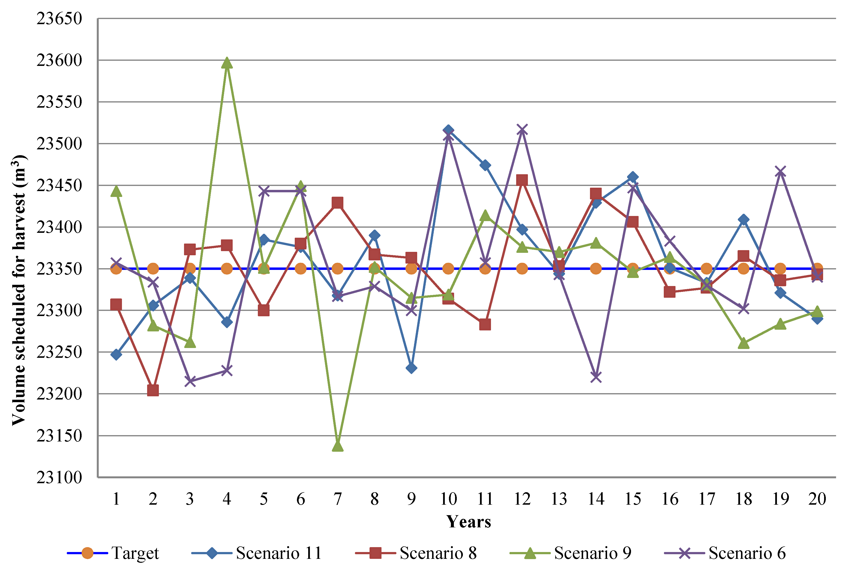
3.1.2. The Results for Volume

The actual volume scheduled for harvest for all 11 scenarios is displayed in Table 7 and the deviations from the volume target (23,350 m3) in Table 8. In addition to the results of volume reference scenario (scenario 11), the results of scenario 8, 9, and 6, which gave better results respectively, are presented in Figure 3.
Similar to the stand area issue, since the stands represent real forest data, the sizes of the stands are all different. Thus, the volume available in a stand is different. Therefore, a solution showing an exact adherence to the target (i.e., with 0 total deviation from the target volume) is likely impossible. For the volume reference scenario (scenario 11), the total deviation from the volume target was 1025 m3 over 20 years. The deviations here ranged from −158 m3 (13th year) to +166 m3 (10th year). The total deviation for 20 years was 2889 m3 under scenario 3, which provided the best result if we evaluate area and volume goals together. The deviations in volume scheduled in scenario 3 ranged from −1.047 m3 (1st year) to 276 m3 (20th year), and the ratio of deviations between the target volume and the scheduled volume varied between −4.48% and +1.18% per year. Again, this deviation is also acceptable in Turkish forest management. In order to better illustrate the results of the linear regeneration model, a map was prepared for scenario 3, which again seemed to be the best solution achieved (Figure 4).
As noted earlier, the 23,350 m3 annual final yield was set as the volume target. If local foresters decide to use the results of scenario 3, they will harvest wood ranging from 22,303 m3 to 23,626 m3 each year. This means the maximum deviation will be 1047 m3 in the first year and the minimum deviation will be only 3 m3 in the third year. If they prefer to use the results of scenario 8, the total volume deviation for 20 years will be only 874 m3. In this case, the regeneration area deviation will be 34.70 ha for 20 years, ranging from 4.05 ha (1st year) to −5.65 ha (16th year). Since this study doesn’t evaluate the economic results of the management scenarios, we are not recommending the local foresters which scenario they would decide to use. However, the largest income source of forest enterprises in Turkey are timber sale revenues. Furthermore, around 90 per cent of the timber they produce comes from the final yield harvest (regeneration). In this case, minimizing the volume deviation is important to meet the needs of the markets in a sustainable manner.

3.2. Comparison of the Actual Regeneration Plan Data with the Results of the Regeneration Model

The actual regeneration plan [56], or detailed silviculture plan, for the study area indicated that over 10 years 881.8 ha of forests would be regenerated, and 209,600 m3 of wood material would be produced (Table 9). This plan was developed using less sophisticated mathematical methods but took into account the growth of the forest. Given this information, we assumed that an area of 88.18 ha (881.8 ha/10 years) and a volume of 20.960 m3 (209,600 m3/10 years) would be scheduled each year, since finer detail was unavailable from the plan. Using scenario 3 of the regeneration model, the total deviation for the first 10 years was 2.1 ha in the area (0.24% of total 10-year regeneration area) and 1959 m3 in volume (0.84% of total 10-year harvest volume). Using the guidance from the actual regeneration plan, the area deviation would be 54.72 ha (6.2% of total regeneration area) from the assumed area target, and the volume deviation would be 20,472 m3 (9.8% of harvest volume) from the assumed volume target (Table 10). This comparison suggests some efficiencies in the regeneration program can be realized using the mathematical programming approach.

4. Discussion

As all of the forests in Turkey are managed using plans prepared in consideration of basic principles such as sustainability, economics, productivity, multi-purpose utilization, protection of biological diversity, aesthetics and protection of other landscape values, and carbon balance, the use of appropriate techniques to achieve management objectives is important. Final yield and intermediate yield harvest plans are included in these management plans. The regeneration activities envisaged in the management plan are carried out according to detailed silviculture plans. In the long run, in order to harvest an equal amount of wood every year, it is necessary to cut a relatively equal area of forest area that will provide this each year. This is only possible in forests that are optimal in terms of their age class distribution. The way to meet these requirements is to establish an equal area of new stands every year and to manage them to the end of the rotation length. This approach, often considered as a regulated forest, should be taken into consideration when preparing the detailed silviculture plans. Furthermore, in accordance with legislation, areas applying a final harvest cannot exceed 25 ha during the greening (green-up) period. It seems impossible to regenerate an equal amount of area each year and to avoid regenerating forest areas larger than 25 ha during the greening period without using decision support systems. We have demonstrated in this case that a mixed integer GP model can be developed to provide efficient plans which can be used as guidance for implementation of activities by field foresters.
With a total of 3620 variables, the linear regeneration model presents a difficult problem. Both this situation and the use of 500 million iterations have greatly extended the Lingo’s computing time. It took a total of 210 h and 4 min and 59 s to run all 11 scenarios. The longest computing time was 35 h and 39 min and 2 s (scenario 4). One of the factors directly affecting the computing time is undoubtedly the number of adjacency constraints, therefore one of the drawbacks of the model was that its long computing time needed to provide proper results when the adjacency constraints are numerous. While there is an inverse relationship between the clear-cut area size and the number of constraints, there is a linear relationship between the green-up period and the number of constraints. Conversely, as the green-up period increases, so generally does the number of constraints. Others recommend that the clear-cut size area be as large as possible and that the green up period is as short as possible to reduce the number of adjacency constraints [57].
We also explored the sensitivity of the model to produce the goals desired, by assessing how the results (harvest volume and regeneration area) changed when the weights applied to the deviational values varied. Managers seeking to locate forest planning solutions may desire that two (or more) goals have the same relative weight, and therefore one challenge to the planner is to determine the normalized weights that are appropriate for the problem [14]. A major issue of debate among the researchers using G concerns the use of normalization techniques to overcome incommensurability. Incommensurability in a weighted GP occurs when deviational variables are represented by different units (ha, m3, km, etc.). The summation of different units may cause an unintentional bias towards the objectives that have a larger magnitude. To overcome this difficulty, it may be necessary to divide each objective by a constant pertaining to that objective, to ensure that all objectives have roughly the same magnitude. Such a constant is known as a normalization constant. There are several normalization methods, each with its own normalization constant [58]. Some of them are percentage normalization [59], Euclidean normalization [60,61], summation normalization [62], and zero–one normalization [63]. However, these normalization methods cannot guarantee that the achieved objectives are consistent with their goals [64]. Therefore, with regard to the type of forestry problem addressed in this research, this area of investigation is still open.

5. Conclusions

In this study, we explained how one might use mixed integer GP in the Turkish forest management planning system to address final harvest issues. This study introduced a new approach to regeneration planning. This study provided an enhancement on previous research in this area as well. The previous research proposed an approach in intermediate harvest planning and stand tending block designation using GP models. The compartments were grouped together to create blocks by minimizing deviation between scheduled compartments. It was the first application of GP in intermediate harvest planning in Turkish forestry. The present study applied a GP model in final yield harvest planning, which is the other main aspect of forest management plans. This study can also be improved by integrating these different models into one comprehensive model to address both problems at the same time. The biggest disadvantage of this study is that it does not take into account natural disturbances such as forest fires, insect and disease outbreaks, and drought and windthrow. This is not unusual, since most forest planning models ignore these issues, due to their high level of uncertainty. However, the process described has some major advantages over the current approaches to develop forest management plans in Turkey. Since the regeneration operations in Turkey are very costly and locating experienced forestry workers to employ to conduct harvesting and regeneration activities is not easy, using this type of model will help forest enterprises to regenerate their forests successfully. Some certainty and regularity of annual production levels can alleviate wood flow fluctuations and help forest enterprises increase their forestry operation efficiency. Further, they will be better positioned to meet the needs of local markets in a sustainable manner by regulating final yield harvest, a major source of income. Should decision-makers consider that this study be useful for forest planning and contribute to Turkish forestry, it would be of great benefit to develop a special matrix generator to solve these (and similar) problems. Finally, the approach can be tested in different planning units and can be employed world-wide in the planning of even-aged forests, primarily pine forests.

Author Contributions

M.D., A.Y., P.B. contributed to the conceptualization and design of the study and developed the goal programming models. M.D. acquired, analyzed, and interpreted the data, solved the model using Lingo 16.0, and wrote the original draft manuscript. A.Y., P.B. supervised the project and reviewed and edited the manuscript. All authors have read and agreed to the published version of the manuscript.

Funding

This research was funded by the Scientific Research Projects Coordination Unit of the Istanbul University-Cerrahpasa (Project number: 20612). This research was supported by the U.S. National Institute of Food and Agriculture McIntire-Stennis research program (Project number: GEOZ-0195-MS).

Acknowledgments

We would like to thank the officials of the Forest Management Planning Department of the General Directorate of Forestry in Turkey for sharing the management plan data and GIS data of the study area. We also thank to the local foresters for sharing the actual silviculture plan of the study area forest.

Conflicts of Interest

The authors declare no conflict of interest. The funders had no role in the design of the study; in the collection, analyses, or interpretation of data; in the writing of the manuscript, or in the decision to publish the results.

References

  1. Zengin, H.; Yeşil, A.; Asan, Ü.; Bettinger, P.; Cieszewski, C.; Siry, J.P. Evolution of modern forest management planning in the Republic of Turkey. J. For. 2013, 111, 239–248. [Google Scholar] [CrossRef] [Green Version]
  2. Bettinger, P.; Sessions, J. Spatial forest planning: To adopt, or not to adopt? J. For. 2003, 101, 24–29. [Google Scholar]
  3. Bettinger, P.; Chung, W. The key literature of, and trends in, forest-level management planning in North America, 1950–2001. Int. Forest. Rev. 2004, 6, 40–50. [Google Scholar] [CrossRef]
  4. Kaya, A.; Bettinger, P.; Boston, K.; Akbulut, R.; Ucar, Z.; Siry, J.; Merry, K.; Cieszewski, C. Optimisation in forest management. Curr. For. Rep. 2016, 2, 1–17. [Google Scholar] [CrossRef] [Green Version]
  5. Eraslan, İ. Forest Management; Faculty of Forestry, Istanbul University: Istanbul, Turkey, 1982. [Google Scholar]
  6. General Directorate of Forestry. Procedures and Principles Regarding the Preparation of Ecosystem Based Functional Forest Management Plans, Communiqué Number: 299; General Directorate of Forestry: Ankara, Turkey, 2014.
  7. Bertomeu, M.; Romero, C. Managing forest biodiversity: A zero-one goal programming approach. Agric. Syst. 2001, 68, 197–213. [Google Scholar] [CrossRef]
  8. Öhman, K. Forest Planning with Consideration to Spatial Relationships. Ph.D. Thesis, Swedish University of Agricultural Sciences, Uppsala, Sweden, 2001. [Google Scholar]
  9. Murray, A.T. Spatial restrictions in harvest scheduling. For. Sci. 1999, 45, 45–52. [Google Scholar]
  10. Liu, W.-Y.; Lin, C.-C.; Su, K.-H. Modelling the spatial forest-thinning planning problem considering carbon sequestration and emissions. For. Policy Econ. 2017, 78, 51–66. [Google Scholar] [CrossRef]
  11. Qin, H.; Dong, L.; Huang, Y. Evaluating the effects of carbon prices on trade-offs between carbon and timber management objectives in forest spatial harvest scheduling problems: A case study from northeast China. Forests 2017, 8, 43. [Google Scholar] [CrossRef] [Green Version]
  12. Augustynczik, A.L.D.; Arce, J.E.; da Silva, A.C.L. Spatial forest harvest planning considering maximum operational areas. Cerne 2015, 21, 649–656. [Google Scholar] [CrossRef] [Green Version]
  13. Tarp, P.; Helles, F. Spatial optimization by simulated annealing and linear programming. Scand. J. For. Res. 1997, 12, 390–402. [Google Scholar] [CrossRef]
  14. Demirci, M.; Bettinger, P. Using mixed integer multi-objective goal programming for stand tending block designation: A case study from Turkey. For. Policy Econ. 2015, 55, 28–36. [Google Scholar] [CrossRef]
  15. Charnes, A.; Cooper, W.W.; Ferguson, R.O. Optimal estimation of executive compensation by linear programming. Manag Sci. 1955, 1, 138–151. [Google Scholar] [CrossRef]
  16. Charnes, A.; Cooper, W.W. Management Models and Industrial Applications of Linear Programming; John Wiley & Sons: New York, NY, USA, 1961; Volume 1, ISBN 978-0-471-14850-0. [Google Scholar]
  17. Ijiri, Y. Management goals and accounting for control. In Studies in Mathematical and Managerial Economics; Theil, H., Ed.; North-Holland Publishing Co.: Amsterdam, The Netherlands, 1965; Volume 3, 191p. [Google Scholar]
  18. Lee, S.M. Goal Programming for Decision Analysis; Auerbach Publishers Inc.: Philadelphia, PA, USA, 1972. [Google Scholar]
  19. Charnes, A.; Cooper, W.W.; Niehaus, R.J. A goal programming model for man power planning. In Management Science in Planning and Control; Blood, J., Ed.; Technical Association of the Pulp and Paper Industry: New York, NY, USA, 1968; pp. 79–93. [Google Scholar]
  20. Charnes, A.; Cooper, W.W.; Niehaus, R.J.; Sholtz, D. An Extended Goal Programming Model Manpower Planning; Management Science Research Report 188; Carnegie-Mellon University, Graduate School of Industrial Administration: Pittsburgh, PA, USA, 1969. [Google Scholar]
  21. Charnes, A.; Cooper, W.W.; Niehaus, R.J. Mathematical Models for Man Power and Personnel Planning; Management Science Research Report 234; Carnegie-Mellon University, Graduate School of Industrial Administration: Pittsburgh, PA, USA, 1971. [Google Scholar]
  22. Charnes, A.; Cooper, W.W.; Niehaus, R.J.; Sholtz, D. Multi-Level Models for Career Management and Resource Planning; Management Science Research Report 256; Carnegie-Mellon University, Graduate School of Industrial Administration: Pittsburgh, PA, USA, 1971. [Google Scholar]
  23. Charnes, A.; Cooper, W.W.; Devoe, J.K.; Learner, D.B.; Reinecke, W. A goal programming model for media planning. Manag. Sci. 1968, 14, 423–430. [Google Scholar] [CrossRef]
  24. Charnes, A.; Cooper, W.W.; Learner, D.B.; Snow, E.F. Note on an application of a goal programming model for media planning. Manag. Sci. 1968, 14, 431–436. [Google Scholar] [CrossRef]
  25. Lee, S.M. Decision analysis through goal programming. Decis. Sci. 1971, 2, 172–180. [Google Scholar]
  26. Lee, S.M.; Lerro, A.J.; McGinnis, B.R. Optimization of tax switching for commercial banks: Comments. J. Money Credit Bank. 1971, 3, 293–303. [Google Scholar] [CrossRef]
  27. Lee, S.M.; Clayton, E.R. A goal programming model for academic resource allocation. Manag. Sci. 1972, 18, 395–408. [Google Scholar] [CrossRef]
  28. Courtney, J.F., Jr.; Klastorin, T.D.; Ruefli, T.W. A goal programming approach to urban-suburban location preferences. Manag. Sci. 1972, 18, 258–268. [Google Scholar] [CrossRef]
  29. Rustagi, K.P. Forest Management Planning for Timber Production: A Goal Programming Approach. Ph.D. Thesis, Yale University, New Haven, CT, USA, 1973. [Google Scholar]
  30. Field, D.B. Goal programming for forest management. For. Sci. 1973, 19, 125–135. [Google Scholar]
  31. Porterfield, R.L. Predicted and Potential Gains from Tree Improvement Programs—A Goal Programming Analysis of Program Efficiency. Ph.D. Thesis, Yale University, New Haven, CT, USA, 1973. [Google Scholar]
  32. Porterfield, R.L. Predicted and Potential Gains from Tree Improvement Programs: A Goal Programming Analysis of Program Efficiency; Technical Report No. 52; North Carolina State University, School of Forest Resources: Raleigh, NC, USA, 1974. [Google Scholar]
  33. Lyon, G. Applications of Goal Programming and Accounting for Control in the Forest Industry; College of Forest Resources, University of Washington: Seattle, WA, USA, 1974; Unpublished work. [Google Scholar]
  34. Romesburg, C.H. Scheduling models for wilderness recreation. J. Environ. Manag. 1974, 2, 159–177. [Google Scholar]
  35. Bell, E.F. Problems with goal programming on a national forest planning unit. In Proceedings of the Systems Analysis and Forest Resource Management Workshop, Athens, GA, USA, 11–13 August 1975; pp. 119–126. [Google Scholar]
  36. Bare, B.; Anholt, B. Selecting Forest Residue Treatment Alternatives Using Goal Programming; General Technical Report PNW-43; USDA Forest Service, Pacific Northwest Forest and Range Experiment Station: Portland, OR, USA, 1976.
  37. Dress, P.E. Forest land use planning-an applications environment for goal programming. In Proceedings of the Systems Analysis and Forest Resource Management Workshop, Athens, GA, USA, 11–13 August 1975; pp. 37–47. [Google Scholar]
  38. Kao, C.; Brodie, J.D. Goal programming for reconciling economic, even flow, and regulation objectives in forest harvest scheduling. Can. J. For. Res. 1979, 9, 525–531. [Google Scholar] [CrossRef]
  39. Field, R.C.; Dress, P.E.; Fortson, J.C. Complementary linear and goal programming procedures for timber harvest scheduling. For. Sci. 1980, 26, 121–133. [Google Scholar]
  40. Kangas, J.; Pukkala, T. A decision theoretic approach applied to goal programming of forest management. Silva Fenn. 1992, 26, 169–176. [Google Scholar] [CrossRef] [Green Version]
  41. Diaz-Balteiro, L.; Romero, C. Modeling timber harvest scheduling problems with multiple criteria: An application in Spain. For. Sci. 1998, 44, 47–57. [Google Scholar]
  42. Mısır, M. Developing a Multi-Objective Model Forest Management Plan Using GIS and Goal Programming (A Case Study of Ormanüstü Planning Unit). Ph.D. Thesis, Karadeniz Technical University, Trabzon, Turkey, 2001. [Google Scholar]
  43. Gómez, T.; Hernández, M.; Molina, J.; León, M.A.; Aldana, E.; Caballero, R. A multi objective model for forest planning with adjacency constraints. Ann. Oper. Res. 2011, 190, 75–92. [Google Scholar] [CrossRef]
  44. Chen, Y.-T.; Zheng, C.; Chang, C.-T. 3-level MCGP: An efficient algorithm for MCGP in solving multi-forest management problems. Scand. J. For. Res. 2011, 26, 457–465. [Google Scholar] [CrossRef]
  45. Chen, Y.-T.; Chang, C.-T. Multi-coefficient goal programming in thinning schedules to increase carbon sequestration and improve forest structure. Ann. For. Sci. 2014, 71, 907–915. [Google Scholar] [CrossRef] [Green Version]
  46. Zengin, H.; Asan, Ü.; Destan, S.; Ünal, M.E.; Yeşil, A.; Bettinger, P.; Değermenci, A.S. Modeling harvest scheduling in multifunctional planning of forests for long term water yield optimization. Nat. Resour. Model. 2015, 28, 59–85. [Google Scholar] [CrossRef]
  47. Augustynczik, A.L.D.; Arce, J.E.; da Silva, A.C.L. Aggregating forest harvesting activities in forest plantations through integer linear programming and goal programming. J. For. Econ. 2016, 24, 72–81. [Google Scholar] [CrossRef]
  48. Bagdon, B.A.; Huang, C.-H.; Dewhurst, S. Managing for ecosystem services in northern Arizona ponderosa pine forests using a novel simulation-to-optimization methodology. Ecol. Model. 2016, 324, 11–27. [Google Scholar] [CrossRef]
  49. Etemad, S.S.; Limaei, S.M.; Olsson, L.; Yousefpour, R. Forest management decision-making using goal programming and fuzzy analytic hierarchy process approaches (case study: Hyrcanian forests of Iran). J. Forest Sci. 2019, 65, 368–379. [Google Scholar] [CrossRef]
  50. Ezquerro, M.; Pardos, M.; Diaz-Baltiero, L. Operational research techniques used for addressing biodiversity objectives into forest management: An overview. Forests 2016, 7, 229. [Google Scholar] [CrossRef] [Green Version]
  51. Álvarez-Miranda, E.; Garcia-Gonzalo, J.; Ulloa-Fierro, F.; Weintraub, A.; Barreiro, S. A multicriteria optimization model for sustainable forest management under climate change uncertainty: An application in Portugal. Eur. J. Oper. Res. 2018, 269, 79–98. [Google Scholar] [CrossRef]
  52. Bertomeu, M.; Romero, C. Forest management optimisation models and habitat diversity: A goal programming approach. J. Oper. Res. Soc. 2002, 53, 1175–1184. [Google Scholar] [CrossRef]
  53. General Directorate of Forestry. Ecosystem Based Functional Forest Management Plan of the Akoren Sub-District; General Directorate of Forestry: Ankara, Turkey, 2014.
  54. General Directorate of Forestry. Communiqué on Technical Principles of Silvicultural Applications; General Directorate of Forestry: Ankara, Turkey, 2014.
  55. Lindo Systems, Inc. Lingo 16.0—Optimization Modeling Software for Linear, Nonlinear, and Integer Programming; Lindo Systems Inc.: Chicago, IL, USA, 2016. [Google Scholar]
  56. Pos Forest District Directorate. Regeneration Plan of the Akoren Forest Sub-District for 2014–2023 (Detailed Silviculture Plan); Adana Forest Regional Directorate, Pos Forest District Directorate: Adana, Turkey, 2015. [Google Scholar]
  57. Walters, K.R.; Feunekes, H.; Cogswell, A.; Cox, E. A forest planning system for solving spatial harvest-scheduling problems. In Proceedings of the Canadian Operations Research Society National Conference, Windsor, ON, Canada, 7–9 June 1999. [Google Scholar]
  58. Tamiz, M.; Jones, D.; Romero, C. Goal programming for decision making: An overview of the current state-of-the-art. Eur. J. Oper. Res. 1998, 111, 569–581. [Google Scholar] [CrossRef]
  59. Romero, C. Handbook of Critical Issues in Goal Programming; Pergamon Press: Oxford, UK, 1991; ISBN 978-1-483-29511-4. [Google Scholar]
  60. De Kluyver, C.A. An exploration of various goal programming formulations—With application to advertising media scheduling. J. Oper. Res. Soc. 1979, 30, 167–171. [Google Scholar]
  61. Wildhelm, W.B. Extensions of goal programming models. Omega 1981, 9, 212–214. [Google Scholar] [CrossRef]
  62. Jones, D.F. The Design and Development of an Intelligent Goal Programming System. Ph.D. Thesis, University of Portsmouth, Portsmouth, UK, 1995. [Google Scholar]
  63. Masud, A.S.; Hwang, C.L. Interactive sequential goal programming. J. Oper. Res. Soc. 1981, 32, 391–400. [Google Scholar] [CrossRef]
  64. Jadidi, O.; Zolfaghari, S.; Cavalieri, S. A new normalized goal programming model for multi-objective problems: A case of supplier selection and order allocation. Int. J. Prod. Econ. 2014, 148, 158–165. [Google Scholar] [CrossRef]
Figure 1. Location of the Akoren Planning Unit and the study area (Turkish pine working circle).
Forests 11 00744 g001
Figure 2. A comparison of the regeneration area achieved using the regeneration model.
Forests 11 00744 g002
Figure 3. A comparison of the scheduled volume achieved using the linear regeneration model.
Forests 11 00744 g003
Figure 4. Regeneration map produced by the regeneration model (scenario 3).
Forests 11 00744 g004
Table 1. Total number of variables and constraints used in the models.
Variables and ConstraintsLinear Regeneration Model
Variables3620
Nonlinear variables0
Integer variables3500
Constraints2767
Nonlinear constraints0
Table 2. Weights for the two objectives.
ScenarioArea Weight
(wi1+ and wi1)
Volume Weight
(wi2+ and wi2)
11.00.0
20.90.1
30.80.2
40.70.3
50.60.4
60.50.5
70.40.6
80.30.7
90.20.8
100.10.9
110.01.0
Table 3. Total solver iterations and elapsed runtime seconds for linear and nonlinear models.
ScenarioTotal Solver IterationsElapsed Runtime
Scenario 1500,000,0017 h 58 min 4 s
Scenario 2500,000,00033 h 25 min 15 s
Scenario 3500,000,0007 h 3 min 34 s
Scenario 4500,000,00135 h 39 min 2 s
Scenario 5500,000,00132 h 14 min 54 s
Scenario 6500,000,0005 h 52 min 12 s
Scenario 7500,000,00130 h 31 min 15 s
Scenario 8500,000,00032 min 48 s
Scenario 9500,000,0005 h 42 min 36 s
Scenario 10500,000,00130 h 36 min 53 s
Scenario 11500,000,00120 h 28 min 26 s
Table 4. Outcomes achieved using the linear regeneration model.
ScenarioDeviations from Goals
Area (ha)Volume (m3)
13.860,613
214.210,968
33.82889
425.47951
524.53790
627.21366
736.13414
834.7874
964.81260
10105.92827
11197.61025
Table 5. Area (ha) scheduled for regeneration for all scenarios when using the regeneration model.
YearScenario
1234567891011
189.588.788.988.689.893.191.792.994.8106.1115.4
288.890.489.190.489.790.289.489.798.589.7130.2
389.087.788.990.094.688.687.689.087.892.799.8
488.988.588.389.089.289.389.492.488.395.789.5
588.888.988.589.285.288.988.987.591.393.790.5
688.889.488.791.488.489.084.991.889.395.991.5
788.988.788.890.287.988.588.488.289.790.888.7
888.989.088.888.289.688.889.388.583.686.099.7
988.787.889.491.789.287.192.387.991.886.990.8
1088.787.388.885.790.187.387.189.188.088.776.2
1189.087.588.886.487.784.986.389.088.789.279.8
1288.991.488.890.288.686.688.785.090.290.590.2
1389.288.488.589.188.190.391.285.683.275.376.9
1488.688.789.189.389.691.884.689.292.090.681.7
1589.188.488.783.288.088.587.490.292.488.580.6
1688.790.088.889.188.291.887.883.290.981.676.8
1789.088.688.988.690.187.988.189.088.395.489.7
1888.888.889.289.388.888.693.392.478.183.074.7
1987.989.689.288.687.588.692.287.882.572.474.3
2088.889.288.888.886.787.288.488.687.684.380.0
Total1777.01777.01777.01777.01777.01777.01777.01777.01777.01777.01777.0
Table 6. Deviations from the area target (ha) when using the regeneration model.
YearScenario
1234567891011
10.65−0.150.05−0.250.954.252.854.055.9517.2526.55
2−0.051.550.251.550.851.350.550.859.650.8541.35
30.15−1.150.051.155.75−0.25−1.250.15−1.053.8510.95
40.05−0.35−0.550.150.350.450.553.55−0.556.850.65
5−0.050.05−0.350.35−3.650.050.05−1.352.454.851.65
6−0.050.55−0.152.55−0.450.15−3.952.950.457.052.65
70.05−0.15−0.051.35−0.95−0.35−0.45−0.650.851.95−0.15
80.050.15−0.05−0.650.75−0.050.45−0.35−5.25−2.8510.85
9−0.15−1.050.552.850.35−1.753.45−0.952.95−1.951.95
10−0.15−1.55−0.05−3.151.25−1.55−1.750.25−0.85−0.15−12.65
110.15−1.35−0.05−2.45−1.15−3.95−2.550.15−0.150.35−9.05
120.052.55−0.051.35−0.25−2.25−0.15−3.851.351.651.35
130.35−0.45−0.350.25−0.751.452.35−3.25−5.65−13.55−11.95
14−0.25−0.150.250.450.752.95−4.250.353.151.75−7.15
150.25−0.45−0.15−5.65−0.85−0.35−1.451.353.55−0.35−8.25
16−0.151.15−0.050.25−0.652.95−1.05−5.652.05−7.25−12.05
170.15−0.250.05−0.251.25−0.95−0.750.15−0.556.550.85
18−0.05−0.050.350.45−0.05−0.254.453.55−10.75−5.85−14.15
19−0.950.750.35−0.25−1.35−0.253.35−1.05−6.35−16.45−14.55
20−0.050.35−0.05−0.05−2.15−1.65−0.45−0.25−1.25−4.55−8.85
Total a3.8014.203.8025.4024.5027.2036.1034.7064.80105.90197.60
a Absolute value of annual deviations.
Table 7. Volume (m3) scheduled for harvest for all scenarios when using the regeneration model.
YearScenarios
1234567891011
119,45422,25322,30322,22822,52423,35723,00623,30723,44323,33423,357
216,79723,38222,99123,38223,19623,33423,12723,20423,28223,20223,403
321,24623,10223,26623,82023,25823,21523,32723,37323,26224,04023,361
421,15123,15523,35323,09223,07523,22823,31423,37823,59723,36123,374
517,62522,33323,32223,22623,09423,44323,44823,30023,35123,12623,363
621,83823,34823,32023,19723,45223,44323,11923,38023,44923,52623,337
720,62722,89523,60323,32723,69423,31723,60023,42923,13823,26423,296
822,52123,95423,44223,88623,08023,32923,21423,36723,35223,51223,426
923,98323,29523,30923,74723,47623,30023,61223,36323,31523,33923,342
1023,02024,94423,37222,02523,46023,51023,63423,31423,31923,37623,516
1126,78124,45523,37523,62423,65523,35723,46423,28323,41423,48923,290
1225,91023,82423,31522,08023,18123,51723,46223,45623,37623,17823,263
1325,74122,93323,18823,66323,35123,34323,17823,35323,37023,34923,192
1423,69121,35223,24323,82423,51023,22023,36723,44023,38123,06223,362
1522,46622,89323,25523,00723,36323,44723,62623,40623,34623,25423,460
1627,03523,45123,43023,54523,34523,38323,39123,32223,36423,28023,391
1724,21824,25723,41323,63423,05723,33023,16923,32723,33123,41523,329
1824,99923,44823,28223,21723,40123,30223,43223,36523,26123,20023,384
1929,77923,38123,33123,34323,25223,46722,91223,33623,28423,50323,332
2035,22123,26923,62623,56823,21023,34023,44423,34323,29923,20723,409
Total474,103465,924465,739465,435465,634467,182466,846467,046466,934467,017467,187
Table 8. Deviations from the volume target (m3) when using the linear regeneration model.
YearScenario
1234567891011
1−3896−1097−1047−1122−8267−344−4393−167
2−655332−35932−154−16−223−146−68−14853
3−2104−248−84470−92−135−2323−8869011
4−2199−1953−258−275−122−36282471124
5−5725−1017−28−124−2569398−501−22413
6−1512−2−30−15310293−2313099176−13
7−2723−455253−23344−3325079−212−86−54
8−82960492536−270−21−13617216276
9633−55−41397126−5026213−35−11−8
10−330159422−1325110160284−36−3126166
1134311105252743057114−6764139−60
122560474−35−1270−16916711210626−172−87
132391−417−1623131−7−172320−1−158
14341−1998−107474160−130179031−28812
15−884−457−95−343139727656−4−96110
16368510180195−53341−2814−7041
1786890763284−293−20−181−23−1965−21
18164998−68−13351−488215−89−15034
19642931−19−7−98117−438−14−66153−18
2011,871−81276218−140−1094−7−51−14359
Total a60,61310,96828897951379013663414874126028271025
a Absolute value of annual deviations.
Table 9. Regeneration data in the forest management plan and detailed silviculture plan.
Forest Management PlanDetailed Silviculture Plan a
Area (ha)Allowable Cut (m3) Area (ha)Allowable Cut (m3)
Regeneration area906.9215,480Natural regeneration344.985,601
Artificial regeneration427.795,604
Regenerated area in 2014109.228,395
Total regeneration881.8209,600
Islet of aging25.15880
General Total906.9215,480
a The detailed silviculture plan covers the first ten years of forest plan implementation (2014–2023).
Table 10. Comparison of the results of scenario 3 of the regeneration model and the silviculture plan.
YearScenario 3 of the Regeneration ModelSilviculture Plan
Area
(ha)
Deviation
(ha)
Volume
(m3)
Deviation
(m3)
Area
(ha)
Deviation
(ha)
Volume
(m3)
Deviation
(m3)
201488.90.0522,303−1047109.221.0228,3957435
201589.10.2522,991−35994.05.8221,196236
201688.90.0523,266−8484.4−3.7818,987−1973
201788.3−0.5523,353382.9−5.2820,751−209
201888.5−0.3523,322−2887.6−0.5823,1712211
201988.7−0.1523,320−3088.70.5220,131−829
202088.8−0.0523,60325383.3−4.8817,083−3877
202188.8−0.0523,4429284.5−3.6820,172−788
202289.40.5523,309−4181.7−6.4818,400−2560
202388.8−0.0523,3722285.5−2.6821,314354
Average88.80.2123,22819688.25.4720,9602047
Total888.22.10232,2811959 a881.854.72209,60020,472 a
a Absolute value of deviations.

