Estimation of the Restored Forest Spatial Structure in Semi-Arid Mine Dumps Using Worldview-2 Imagery
Abstract
1. Introduction
2. Materials and Methods
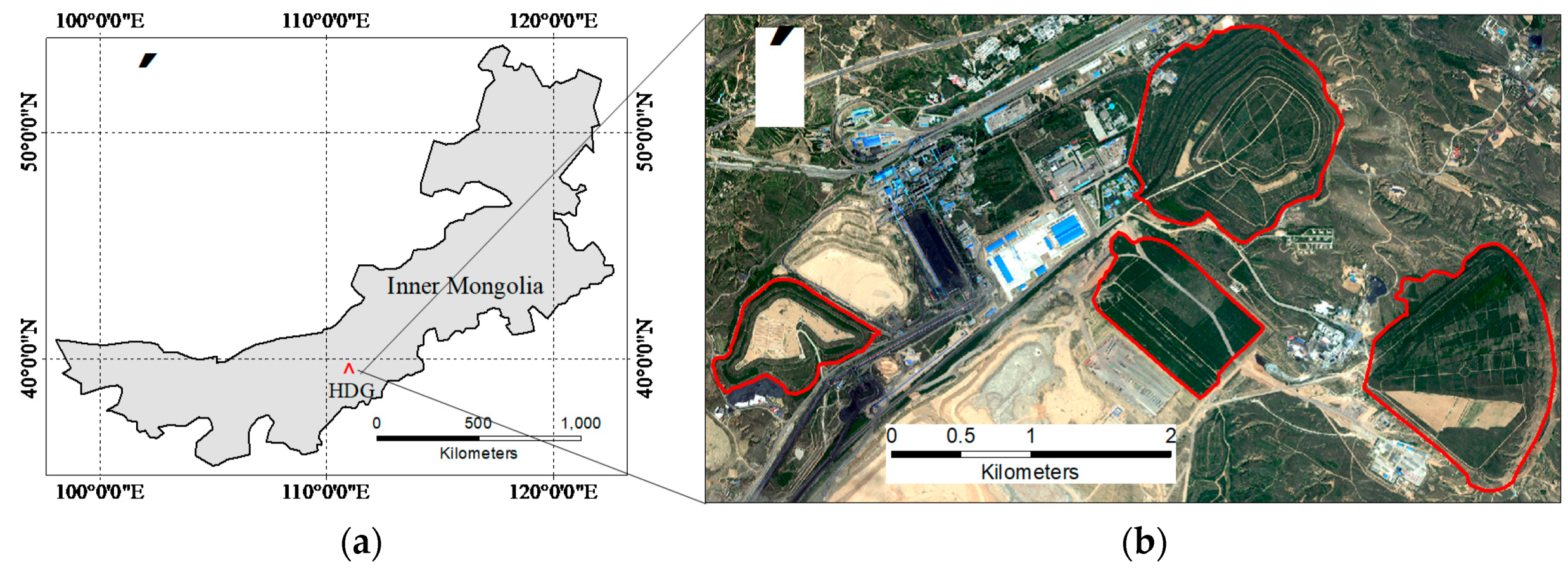
2.1. Study Area
2.2. Forest Spatial Structure
2.2.1. Definition of Spatial Structure Units
2.2.2. Construction of Index System
2.3. Field Measurements
2.4. Remote Sensing Data and Pre-Processing
2.5. Image Feature Extraction
2.5.1. Construction of Feature Factor Library
2.5.2. Screening of Feature Factor Library
2.6. Modeling
2.6.1. MEA-BP Neural Network Estimation Model
- Intermediate layer selectionChoosing the appropriate number of intermediate layers for the neural network can improve the prediction accuracy of the network and reduce the number of prediction errors. Here, a neural network structure with one intermediate layer was established based on the network convergence speed and data volume.
- Input layer nodesAccording to the filtering result of the feature factor library, the number of input layer nodes was set to ten, and the specific input parameters were the parameter factors of the feature factor set after screening. One output layer was employed, which contains the SSPs to be extracted.
- Determination of the number of nodes in the hidden layerThe hidden layer nodes were determined according to an empirical formula, and the initial structural group was constructed using Equation (8):where h, n, and m are the number of nodes in the hidden, input, and output layers, respectively, and a is a constant in the range of [1,10]. The optimal number of nodes in the hidden layer was determined to be 12 by trial-and-error.
- Activation functionAiming at the three-layer network structure of this study, with one output layer, the Sigmoid function (Equation (9)) was selected as the intermediate layer activation function:
- MEA parameter setting and data pre-processingThe initial population size was set to 200, and both the superior and temporary subpopulations were five. The normalized data were input into the model to reduce network errors.
2.6.2. Regression Estimation Model
2.7. Evaluation of Accuracy
3. Results
3.1. Descriptive Statistics of Sample Points
3.2. The Feature Factors for Models
3.2.1. Feature Factors for Regression Model
3.2.2. Feature Factors for MEA-BP Neural Network Model
3.3. The Performance of Estimation
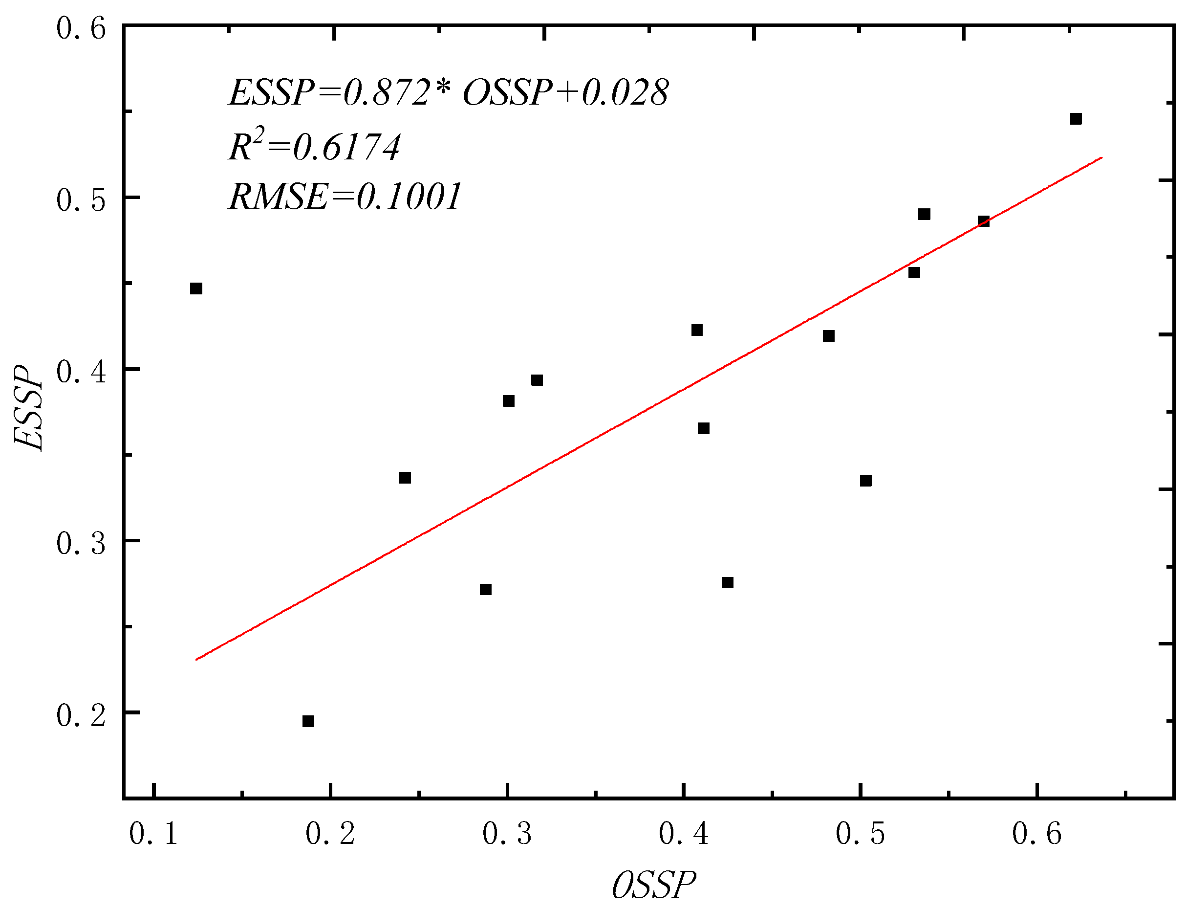
3.3.1. Regression Model
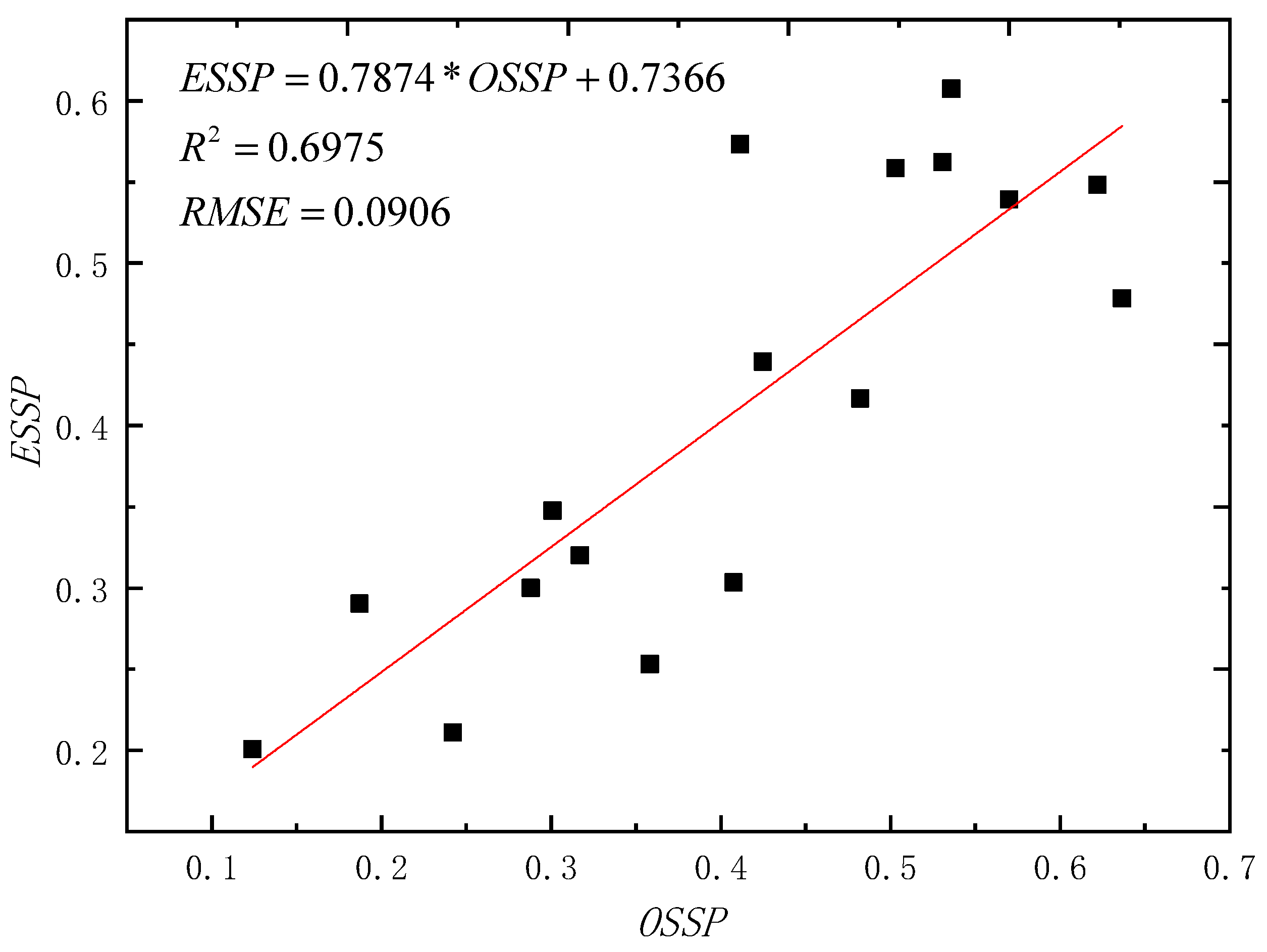
3.3.2. MEA-BP Neural Network
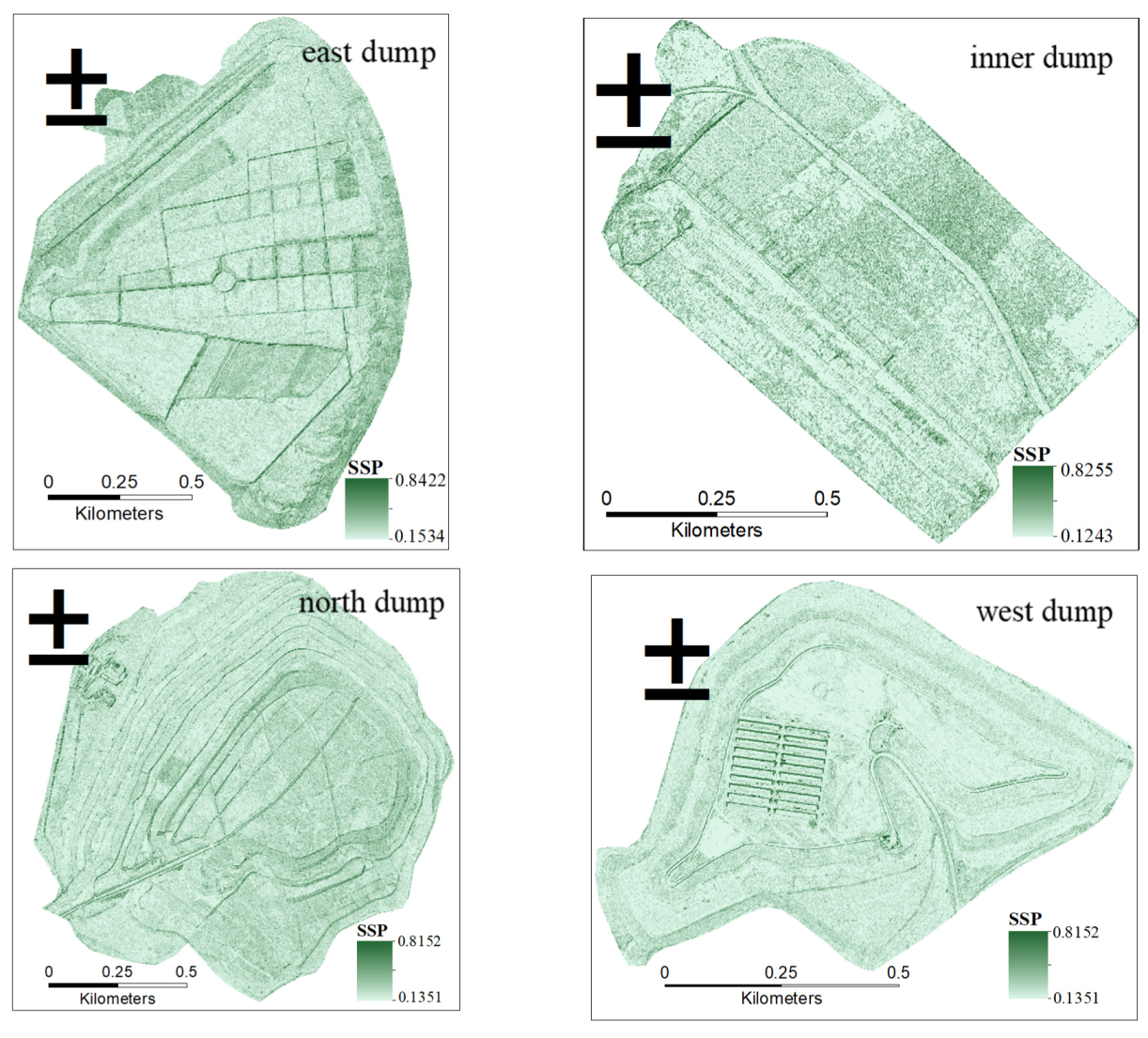
3.4. Estimated Spatial Structure
4. Discussion
4.1. Variation of Spatial Structure
4.2. Limitations and Future Work
5. Conclusions
Author Contributions
Funding
Acknowledgments
Conflicts of Interest
References
- Yang, Y.; Erskine, P.D.; Lechner, A.M.; Mulligan, D.; Zhang, S.; Wang, Z. Detecting the dynamics of vegetation disturbance and recovery in surface mining area via Landsat imagery and LandTrendr algorithm. J. Clean. Prod. 2018, 178, 353–362. [Google Scholar] [CrossRef]
- Iizuka, K.; Yonehara, T.; Itoh, M.; Kosugi, Y. Estimating Tree Height and Diameter at Breast Height (DBH) from Digital Surface Models and Orthophotos Obtained with an Unmanned Aerial System for a Japanese Cypress (Chamaecyparis obtusa) Forest. Remote Sens. 2018, 10, 13. [Google Scholar] [CrossRef]
- Randlane, T.; Tullus, T.; Saag, A.; Lutter, R.; Tullus, A.; Helm, A.; Tullus, H.; Partel, M. Diversity of lichens and bryophytes in hybrid aspen plantations in Estonia depends on landscape structure. Can. J. For. Res. 2017, 47, 1202–1214. [Google Scholar] [CrossRef]
- Wernsdorfer, H.; Colin, A.; Bontemps, J.D.; Chevalier, H.; Pignard, G.; Caurla, S.; Leban, J.M.; Herve, J.C.; Fournier, M. Large-scale dynamics of a heterogeneous forest resource are driven jointly by geographically varying growth conditions, tree species composition and stand structure. Ann. Sci. 2012, 69, 829–844. [Google Scholar] [CrossRef]
- Dong, L.; Wei, H.; Liu, Z. Optimizing Forest Spatial Structure with Neighborhood-Based Indices: Four Case Studies from Northeast China. Forests 2020, 11, 413. [Google Scholar] [CrossRef]
- Bergseng, E.; Ask, J.A.; Framstad, E.; Gobakken, T.; Solberg, B.; Hoen, H.F. Biodiversity protection and economics in long term boreal forest management—A detailed case for the valuation of protection measures. For. Policy Econ. 2012, 15, 12–21. [Google Scholar] [CrossRef]
- Ozdemir, I.; Karnieli, A. Predicting forest structural parameters using the image texture derived from Worldview-2 multispectral imagery in a dryland forest, Israel. Int. J. Appl. Earth Obs. Geoinf. 2011, 13, 701–710. [Google Scholar] [CrossRef]
- Mitchell, M.G.E.; Wu, D.; Johansen, K.; Maron, M.; McAlpine, C.; Rhodes, J.R.; Lee, T.M. Landscape structure influences urban vegetation vertical structure. J. Appl. Ecol. 2016, 53, 1477–1488. [Google Scholar] [CrossRef]
- Leempoel, K.; Bourgeois, C.; Zhang, J.; Wang, J.; Dahdouh-Guebas, F.; Bogaert, J. Spatial heterogeneity in the mangrove vegetation structure in the Zhanjiang Mangrove National Nature Reserve (China): An approach using remote sensing(GeoEye-1 iamgery) and GIS-analysis. VLIZ Spec. Publ. 2012, 43, 68–76. [Google Scholar]
- Ferreira, J.N.; Bustamante, M.; Garcia-Montiel, D.C.; Caylor, K.K.; Davidson, E.A. Spatial variation in vegetation structure coupled to plant available water determined by two-dimensional soil resistivity profiling in a Brazilian savanna. Oecologia 2007, 153, 417–430. [Google Scholar] [CrossRef]
- Claverie, M.; Demarez, V.; Duchemin, B.; Hagolle, O.; Ducrot, D.; Marais-Sicre, C.; Dejoux, J.-F.; Huc, M.; Keravec, P.; Béziat, P.; et al. Maize and sunflower biomass estimation in southwest France using high spatial and temporal resolution remote sensing data. Remote Sens. Environ. 2012, 124, 844–857. [Google Scholar] [CrossRef]
- White, J.C.; Coops, N.C.; Wulder, M.A.; Vastaranta, M.; Hilker, T.; Tompalski, P. Remote Sensing Technologies for Enhancing Forest Inventories: A Review. Can. J. Remote Sens. 2016, 42, 619–641. [Google Scholar] [CrossRef]
- Bao, N.; Lechner, A.M.; Johansen, K.; Ye, B. Object-based classification of semi-arid vegetation to support mine rehabilitation and monitoring. J. Appl. Remote Sens. 2014, 8. [Google Scholar] [CrossRef]
- Luhar, M.; Rominger, J.; Nepf, H. Interaction between flow, transport and vegetation spatial structure. Environ. Fluid Mech. 2008, 8, 423–439. [Google Scholar] [CrossRef]
- Mohseni, N.; Sepehr, A.; Hosseinzadeh, S.R.; Golzarian, M.R.; Shabani, F. Variations in spatial patterns of soil-vegetation properties over subsidence-related ground fissures at an arid ecotone in northeastern Iran. Environ. Earth Sci. 2017, 76, 13. [Google Scholar] [CrossRef]
- Diouf, A.; Barbier, N.; Mahamane, A.; Lejoly, J.; Saadou, M.; Bogaert, J. Characterization of the spatial structure of woody species in “gapped bush” vegetation in southwest Niger. Can. J. For. Res. 2010, 12, 1201–1220. [Google Scholar] [CrossRef]
- Muchoney, D.; Strahler, A. Regional vegetation mapping and direct land surface parameterization from remotely sensed and site data. Int. J. Remote Sens. 2002, 23, 1125–1142. [Google Scholar] [CrossRef]
- Mallinis, G.; Mitsopoulos, I.; Chrysafi, I. Evaluating and comparing Sentinel 2A and Landsat-8 Operational Land Imager (OLI) spectral indices for estimating fire severity in a Mediterranean pine ecosystem of Greece. Giscience Remote Sens. 2017, 55, 1–18. [Google Scholar] [CrossRef]
- Kazar, S.A.; Warner, T.A. Assessment of carbon storage and biomass on minelands reclaimed to grassland environments using Landsat spectral indices. J. Appl. Remote Sens. 2013, 7. [Google Scholar] [CrossRef]
- Zhang, C.; Ren, H.; Huang, Z.; Li, J.; Qin, Q.; Zhang, T.; Sun, Y. Assessment of the application of copper stress vegetation index on Hyperion image in Dexing Copper Mine, China. J. Appl. Remote Sens. 2019, 13. [Google Scholar] [CrossRef]
- Phillip, M.K.; Stuart, P.; Peter, E. Fire Severity and Vegetation Recovery on Mine Site Rehabilitation Using Worldview-3 Imagery. Fire 2018, 1, 22. [Google Scholar]
- Mateo-Sanchis, A.; Munoz-Mari, J.; Perez-Suay, A.; Camps-Valls, G. Warped Gaussian Processes in Remote Sensing Parameter Estimation and Causal Inference. IEEE Geosci. Remote Sens. Lett. 2018, 15, 1647–1651. [Google Scholar] [CrossRef]
- Mettas, C.; Agapiou, A.; Themistocleous, K.; Neocleous, K.; Hadjimitsis, D.G. Detection of asphalt pavement cracks using remote sensing techniques. In Proceedings of the Remote Sensing Technologies And Applications In Urban Environments, Edinburgh, UK, 26–27 September 2016; Erbertseder, T., Esch, T., Chrysoulakis, N., Eds.; SPIE: Bellingham, WA, USA, 2016; Volume 10008. [Google Scholar]
- Zeng, X.; Liu, Z.; He, C.; Ma, Q.; Wu, J. Detecting surface coal mining areas from remote sensing imagery: An approach based on object-oriented decision trees. J. Appl. Remote Sens. 2017, 11. [Google Scholar] [CrossRef]
- Kaplan, G.; Avdan, U. Monthly Analysis of Wetlands Dynamics Using Remote Sensing Data. ISPRS Int. J. Geo-Inf. 2018, 7, 411. [Google Scholar] [CrossRef]
- Gasparovic, M.; Rumora, L.; Miler, M.; Medak, D. Effect of fusing Sentinel-2 and Worldview-4 imagery on the various vegetation indices. J. Appl. Remote Sens. 2019, 13. [Google Scholar] [CrossRef]
- Kayet, N.; Pathak, K.; Chakrabarty, A.; Sahoo, S. Urban heat island explored by co-relationship between land surface temperature vs multiple vegetation indices. Spat. Inf. Res. 2016, 24, 515–529. [Google Scholar] [CrossRef]
- Kiala, Z.; Odindi, J.; Mutanga, O.; Peerbhay, K. Comparison of partial least squares and support vector regressions for predicting leaf area index on a tropical grassland using hyperspectral data. J. Appl. Remote Sens. 2016, 10. [Google Scholar] [CrossRef]
- Mutowo, G.; Mutanga, O.; Masocha, M. Mapping foliar N in miombo woodlands using sentinel-2 derived chlorophyll and structural indices. J. Appl. Remote Sens. 2018, 12. [Google Scholar] [CrossRef]
- Kozoderov, V.V.; Dmitriev, E.V.; Melnik, P.G.; Donskoi, S.A. Evaluation of the Species Composition and the Biological Productivity of Forests Based on Remote Sensing Data with High Spatial and Spectral Resolution. Izv. Atmos. Ocean. Phys. 2018, 54, 1374–1380. [Google Scholar] [CrossRef]
- DeTar, W.R.; Penner, J.V. Airborne remote sensing used to estimate percent canopy cover and to extract canopy temperature from scene temperature in cotton. Trans. Asabe 2007, 50, 495–506. [Google Scholar] [CrossRef]
- Grosse-Stoltenberg, A.; Hellmann, C.; Werner, C.; Oldeland, J.; Thiele, J. Evaluation of Continuous VNIR-SWIR Spectra versus Narrowband Hyperspectral Indices to Discriminate the Invasive Acacia longifolia within a Mediterranean Dune Ecosystem. Remote Sens. 2016, 8, 334. [Google Scholar] [CrossRef]
- Wang, Z.; Lechner, A.M.; Yang, Y.; Baumgartl, T.; Wu, J. Mapping the cumulative impacts of long-term mining disturbance and progressive rehabilitation on ecosystem services. Sci. Total Environ. 2020, 717, 137214. [Google Scholar] [CrossRef] [PubMed]
- Zhang, M.; Wang, J.; Feng, Y. Temporal and spatial change of land use in a large-scale opencast coal mine area: A complex network approach. Land Use Policy 2019, 86, 375–386. [Google Scholar] [CrossRef]
- Elhag, M.; Gitas, I.; Othman, A.; Bahrawi, J.; Gikas, P. Assessment of Water Quality Parameters Using Temporal Remote Sensing Spectral Reflectance in Arid Environments, Saudi Arabia. Water 2019, 11, 556. [Google Scholar] [CrossRef]
- Lausch, A.; Pause, M.; Merbach, I.; Gwillym-Margianto, S.; Schulz, K.; Zacharias, S.; Seppelt, R. Scale-specific Hyperspectral Remote Sensing Approach in Environmental Research. Photogramm. Fernerkund. Geoinf. 2012, 589–601. [Google Scholar] [CrossRef]
- Weissteiner, C.J.; Strobl, P.; Sommer, S. Assessment of status and trends of olive farming intensity in EU-Mediterranean countries using remote sensing time series and land cover data. Ecol. Indic. 2011, 11, 601–610. [Google Scholar] [CrossRef]
- Zhan, Y.; Su, Y.; Huang, J.; Ye, F.; Zhang, C. Mineral recognition mapping using measured spectra based on classification and regression tree. J. Appl. Remote Sens. 2016, 10. [Google Scholar] [CrossRef]
- Zhou, C.; Wang, B.; Wang, W.; Zhao, P.; Li, W. Stability evaluation of different forest communities in Huanglongshan mountain based on the spatial structure index. J. Cent. South Univ. For. Technol. 2018, 38, 76–82. [Google Scholar] [CrossRef]
- Verrelst, J.; Rivera, J.P.; Gitelson, A.; Delegido, J.; Moreno, J.; Camps-Valls, G. Spectral band selection for vegetation properties retrieval using Gaussian processes regression. Int. J. Appl. Earth Obs. Geoinf. 2016, 52, 554–567. [Google Scholar] [CrossRef]
- Dandois, J.P.; Ellis, E.C. High spatial resolution three-dimensional mapping of vegetation spectral dynamics using computer vision. Remote Sens. Environ. 2013, 136, 259–276. [Google Scholar] [CrossRef]
- Keshava, N.; Mustard, J.F. Spectral unmixing. IEEE Signal Process. Mag. 2002, 19, 44–57. [Google Scholar] [CrossRef]
- Schmidt, K.S.; Skidmore, A.K. Spectral discrimination of vegetation types in a coastal wetland. Remote Sens. Environ. 2003, 85, 92–108. [Google Scholar] [CrossRef]
- Verrelst, J.; Rivera, J.P.; Leonenko, G.; Alonso, L.; Moreno, J. Optimizing LUT-Based RTM Inversion for Semiautomatic Mapping of Crop Biophysical Parameters from Sentinel-2 and-3 Data: Role of Cost Functions. IEEE Trans. Geosci. Remote Sens. 2014, 52, 257–269. [Google Scholar] [CrossRef]
- Wallace, A.; Nichol, C.; Woodhouse, I. Recovery of Forest Canopy Parameters by Inversion of Multispectral LiDAR Data. Remote Sens. 2012, 4, 509–531. [Google Scholar] [CrossRef]
- Mutanga, O.; Adam, E.; Cho, M.A. High density biomass estimation for wetland vegetation using Worldview-2 imagery and random forest regression algorithm. Int. J. Appl. Earth Obs. Geoinf. 2012, 18, 399–406. [Google Scholar] [CrossRef]
- Vastaranta, M.; Yu, X.; Luoma, V.; Karjalainen, M.; Saarinen, N.; Wulder, M.A.; White, J.C.; Persson, H.J.; Hollaus, M.; Yrttimaa, T.; et al. Aboveground forest biomass derived using multiple dates of Worldview-2 stereo-imagery: Quantifying the improvement in estimation accuracy. Int. J. Remote Sens. 2018, 39, 8766–8783. [Google Scholar] [CrossRef]
- Yakimov, V.N. General problems of metrology and measurement technique—The structural design of digital correlometers for operational correlation analysis based on sign-function analog-stochastic quantization. Meas. Tech. 2007, 50, 356–363. [Google Scholar] [CrossRef]
- Breiman, L. Random Forests. Mach. Learn. 2001, 45, 5–32. [Google Scholar] [CrossRef]
- Zhang, Y.Q.; Cao, G.; Li, X.S.; Wang, B.S. Cascaded Random Forest for Hyperspectral Image Classification. IEEE J. Sel. Top. Appl. Earth Obs. Remote Sens. 2018, 11, 1082–1094. [Google Scholar] [CrossRef]
- Maren, A.; Jones, D.; Franklin, S. Configuring and optimizing the back-propagation network. In Handbook of Neural Computing Applications; Elsevier: Amsterdam, The Netherlands, 1990; pp. 237–250. [Google Scholar] [CrossRef]
- Wang, W.; Tang, R.; Li, C.; Liu, P.; Luo, L. A BP neural network model optimized by Mind Evolutionary Algorithm for predicting the ocean wave heights. Ocean Eng. 2018, 162, 98–107. [Google Scholar] [CrossRef]
- Jagodziński, A.M.; Zasada, M.; Bronisz, K.; Bronisz, A.; Bijak, S. Biomass conversion and expansion factors for a chronosequence of young naturally regenerated silver birch (Betula pendula Roth) stands growing on post-agricultural sites. For. Ecol. Manag. 2017, 384, 208–220. [Google Scholar] [CrossRef]
- Wing, B.M.; Ritchie, M.W.; Boston, K.; Cohen, W.B.; Gitelman, A.; Olsen, M.J. Prediction of understory vegetation cover with airborne lidar in an interior ponderosa pine forest. Remote Sens. Environ. 2012, 124, 730–741. [Google Scholar] [CrossRef]
- John, R.; Dalling, J.W.; Harms, K.E.; Yavitt, J.B.; Stallard, R.F.; Mirabello, M.; Hubbell, S.P.; Valencia, R.; Navarrete, H.; Vallejo, M.; et al. Soil nutrients influence spatial distributions of tropical tree species. Proc. Natl. Acad. Sci. USA 2007, 104, 864–869. [Google Scholar] [CrossRef] [PubMed]
- Caynes, R.J.C.; Mitchell, M.G.E.; Wu, D.S.; Johansen, K.; Rhodes, J.R. Using high-resolution LiDAR data to quantify the three-dimensional structure of vegetation in urban green space. Urban Ecosyst. 2016, 19, 1749–1765. [Google Scholar] [CrossRef]
- Owers, C.J.; Rogers, K.; Woodroffe, C.D. Identifying spatial variability and complexity in wetland vegetation using an object-based approach. Int. J. Remote Sens. 2016, 37, 4296–4316. [Google Scholar] [CrossRef]
- Lim, K.; Treitz, P.; Wulder, M.; St-Onge, B.; Flood, M. LiDAR remote sensing of forest structure. Prog. Phys. Geogr. 2003, 27, 88–106. [Google Scholar] [CrossRef]
- Béland, M.; Baldocchi, D.D.; Widlowski, J.-L.; Fournier, R.A.; Verstraete, M.M. On seeing the wood from the leaves and the role of voxel size in determining leaf area distribution of forests with terrestrial LiDAR. Agric. For. Meteorol. 2014, 184, 82–97. [Google Scholar] [CrossRef]
- Choi, H.; Song, Y.; Jang, Y. Urban Forest Growth and Gap Dynamics Detected by Yearly Repeated Airborne Light Detection and Ranging (LiDAR): A Case Study of Cheonan, South Korea. Remote Sens. 2019, 11, 1551. [Google Scholar] [CrossRef]
- Mulverhill, C.; Coops, N.C.; White, J.C.; Tompalski, P.; Marshall, P.L. Structural development following stand-replacing disturbance in a boreal mixedwood forest. For. Ecol. Manag. 2019, 453. [Google Scholar] [CrossRef]
- Szostak, M.; Pietrzykowski, M.; Likus-Cieslik, J. Reclaimed Area Land Cover Mapping Using Sentinel-2 Imagery and LiDAR Point Clouds. Remote Sens. 2020, 12, 261. [Google Scholar] [CrossRef]
- Koska, B.; Jirka, V.; Urban, R.; Kremen, T.; Hesslerov, P.; Jon, J.; Pospsil, J.; Fogl, M. Suitability, characteristics, and comparison of an airship UAV with lidar for middle size area mapping. Int. J. Remote Sens. 2017, 38, 2973–2990. [Google Scholar] [CrossRef]
- Urban, R.; Koska, B.; Moudry, V.; Solsky, M.; Sgem. Terrain of Post Mining Site from Airship Lidar. In Proceedings of the Informatics, Geoinformatics And Remote Sensing Conference Proceedings, Sgem 2016, Vol II, Albena, Bulgaria, 30 June–6 July 2016; pp. 577–584. [Google Scholar]
- Ostrowski, W.; Górski, K.; Pilarska, M.; Salach, A.; Bakuła, K. Comparison of the laser scanning solutions for the unmanned aerial vehicles. Arch. Photogramm. Cart. Remote Sens. 2017, 29, 101–123. [Google Scholar] [CrossRef]

| Index | 0 | 0.25 | 0.5 | 0.75 | 1 |
|---|---|---|---|---|---|
| M |  Four adjacent trees are same species as the reference tree (no mixing) |  Three adjacent trees are same species as the reference tree (weak mixing) |  Two adjacent trees are same species as the reference tree (medium mixing) |  One adjacent tree is same species as the reference tree (strong mixing) |  No adjacent trees are same species as the reference tree (extreme mixing) |
| D |  Five adjacent trees have the same properties (no difference) |  Two different properties (light difference) |  Three different properties (medium difference) |  Four different properties (strong difference) |  Five different properties (major difference) |
| C |  No adjacent trees overlap with the reference crown (very sparse) |  One adjacent tree overlaps with the reference crown (relative sparse) |  Two adjacent trees overlap with the reference crown (medium sparse) |  Three adjacent trees overlap with the reference crown (relative dense) |  our adjacent trees overlap with the reference crown (very dense) |
| W |  Four angles are less than the standard angle (Very uneven distribution) |  Three angles are less than the standard angle (uneven distribution) |  Two angles are less than the standard angle (random distribution) |  One angle is less than the standard angle (even distribution) |  No angles are less than the standard angle (Very even distribution) |
| U/H |  No adjacent trees are smaller than reference trees (absolute disadvantage) |  One adjacent tree is smaller than reference trees (disadvantage) |  Two adjacent trees are smaller than reference trees (moderate) |  Three adjacent trees are smaller than reference trees (Sub-advantage) |  Four adjacent trees are smaller than reference trees (absolute advantage) |
| Vegetation Index | Expression |
|---|---|
| Soil Adjusted Vegetation Index (SAVI) | |
| Ratio Vegetation Index (RVI) | |
| Enhanced Vegetation Index (EVI) | |
| Difference Vegetation Index (DVI) | |
| Normalized Difference Vegetation Index (NDVI) | |
| Modified Soil Adjusted Vegetation Index (MSAVI) |
| Data Set | N1 | Maximum | Minimum | Mean | Standard Deviation | Coefficient of Variation |
|---|---|---|---|---|---|---|
| Training set | 35 | 0.792 | 0.375 | 0.538 | 0.139 | 0.258 |
| Test set | 17 | 0.750 | 0.333 | 0.522 | 0.136 | 0.260 |
| Feature Factors | B8T3R (x1) | B7T3M (x2) | B5T3S (x3) | NIR1 (x4) |
|---|---|---|---|---|
| Correlation coefficient | 0.535 | 0.624 | 0.567 | 0.540 |
| Significance level | 0.05 | 0.001 | 0.05 | 0.05 |
| Spvi | T3 | T7 | T9 | T11 | T13 | T15 | T17 |
|---|---|---|---|---|---|---|---|
| NDVI | B3T3D | B3T7R | B3T9R | B3T11R | B3T13R | B3T15R | B3T17R |
| RVI | B6T3E | B6T7E | B5T9E | B5T11E | B6T13R | B6T15R | B2T17R |
| SAVI | RVI | B5T7E | B5T9C | B2T11R | B7T13V | B2T15R | B6T17R |
| MASVI | NDVI | B6T7R | B2T9V | B7T11V | B5T13V | B7T15H | B4T17R |
| EVI | SAVI | B5T7S | B5T9V | B5T11V | B7T13E | B5T15V | B7T17H |
| Blue | EVI | B5T7C | B2T9S | B6T11R | B4T13R | B4T15R | B7T17E |
| Coast blue | B3T3R | B5T7V | B6T9R | B2T11S | B7T13S | B6T15S | B7T17S |
| DVI | B6T3S | B2T7S | B5T9H | B8T11V | B5T13C | B7T15V | B7T17D |
| Nir2 | B8T3E | B2T7E | B5T9E | B2T11V | B7T13D | B7T15E | B6T17E |
| Red | B8T3S | B5T7H | B2T9C | B7T11S | B5T13E | B6T15E | B5T17E |
| Sum of Squares | df | Variance | F | p | |
|---|---|---|---|---|---|
| Regression | 0.206 | 4 | 0.058 | 3.938 | 0.011 |
| Residual | 0.214 | 30 | 0.015 | ||
| Sum | 0.420 | 34 |
| Spvi | T3 | T7 | T9 | T11 | T13 | T15 | T17 | |
|---|---|---|---|---|---|---|---|---|
| −0.4679 | 0.6235 | −0.0667 | 0.4621 | 0.2389 | 0.3972 | 0.4507 | 0.3913 | |
| 0.1461 | 0.0906 | 0.5265 | 0.1698 | 0.2140 | 0.1803 | 0.1452 | 0.1461 |
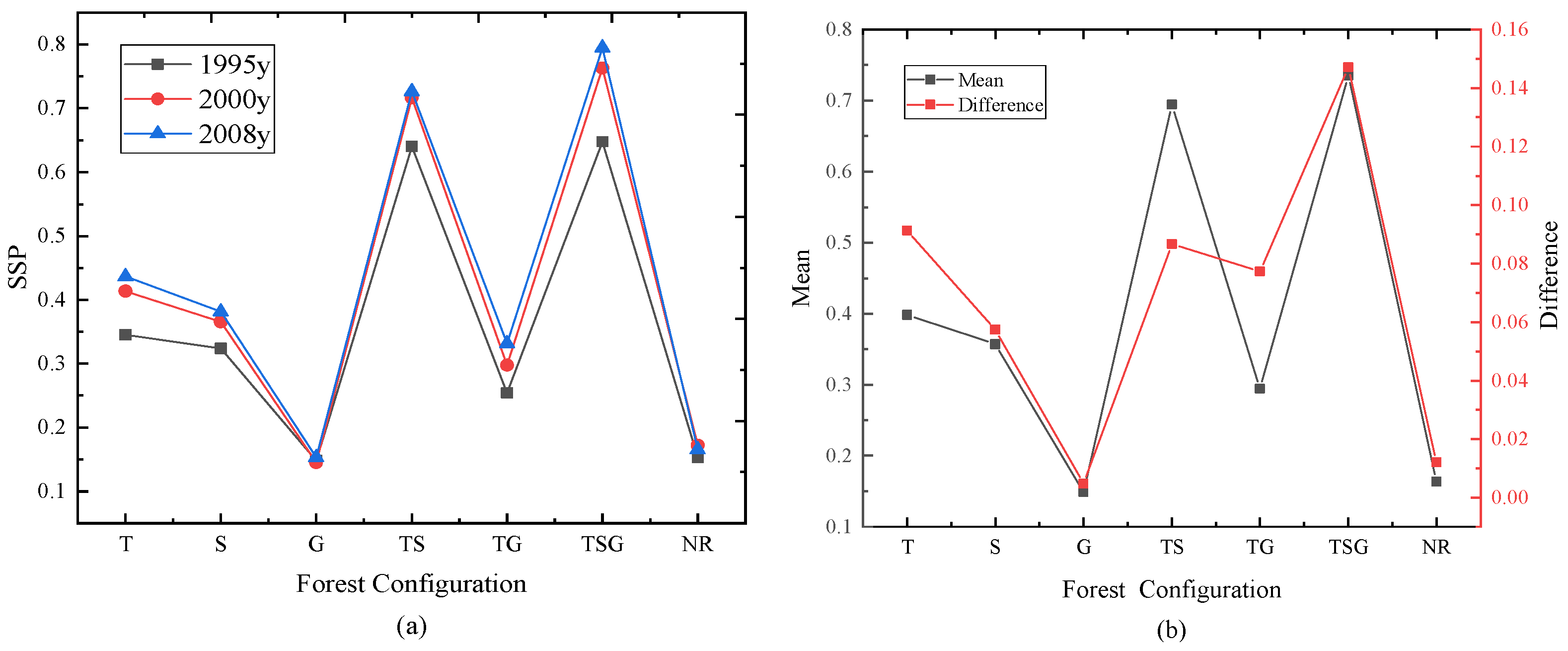
| SSP Year | Reclamation Years | Mean | Difference | ||
|---|---|---|---|---|---|
| 1995 | 2000 | 2008 | |||
| T | 0.3453 | 0.4135 | 0.4366 | 0.39844 | 0.09133 |
| S | 0.3241 | 0.3654 | 0.3815 | 0.35702 | 0.05744 |
| G | 0.1484 | 0.1451 | 0.1531 | 0.14887 | 0.00470 |
| TS | 0.6398 | 0.7166 | 0.7265 | 0.69428 | 0.08670 |
| TG | 0.2541 | 0.2975 | 0.3315 | 0.29435 | 0.07740 |
| TSG | 0.6475 | 0.7632 | 0.7946 | 0.73509 | 0.14708 |
| NR | 0.1534 | 0.1721 | 0.1654 | 0.16363 | 0.01200 |
© 2020 by the authors. Licensee MDPI, Basel, Switzerland. This article is an open access article distributed under the terms and conditions of the Creative Commons Attribution (CC BY) license (http://creativecommons.org/licenses/by/4.0/).
Share and Cite
Zhu, X.; Zhou, Y.; Yang, Y.; Hou, H.; Zhang, S.; Liu, R. Estimation of the Restored Forest Spatial Structure in Semi-Arid Mine Dumps Using Worldview-2 Imagery. Forests 2020, 11, 695. https://doi.org/10.3390/f11060695
Zhu X, Zhou Y, Yang Y, Hou H, Zhang S, Liu R. Estimation of the Restored Forest Spatial Structure in Semi-Arid Mine Dumps Using Worldview-2 Imagery. Forests. 2020; 11(6):695. https://doi.org/10.3390/f11060695
Chicago/Turabian StyleZhu, Xiaoxiao, Yongli Zhou, Yongjun Yang, Huping Hou, Shaoliang Zhang, and Run Liu. 2020. "Estimation of the Restored Forest Spatial Structure in Semi-Arid Mine Dumps Using Worldview-2 Imagery" Forests 11, no. 6: 695. https://doi.org/10.3390/f11060695
APA StyleZhu, X., Zhou, Y., Yang, Y., Hou, H., Zhang, S., & Liu, R. (2020). Estimation of the Restored Forest Spatial Structure in Semi-Arid Mine Dumps Using Worldview-2 Imagery. Forests, 11(6), 695. https://doi.org/10.3390/f11060695


