Article

Characterizing over Four Decades of Forest Disturbance in Minnesota, USA

by
Jody C. Vogeler
1,2,*,
Robert A. Slesak
3,4,
Patrick A. Fekety
1 and
Michael J. Falkowski
1,2
1
Natural Resources Ecology Laboratory, Colorado State University, Fort Collins, CO 80523, USA
2
Department of Ecosystem Science and Sustainability, Colorado State University, Fort Collins, CO 80523, USA
3
Department of Forest Resources, University of Minnesota, Saint Paul, MN 55108, USA
4
Minnesota Forest Resources Council, Saint Paul, MN 55108, USA
*
Author to whom correspondence should be addressed.
Forests 2020, 11(3), 362; https://doi.org/10.3390/f11030362
Submission received: 4 March 2020 / Revised: 20 March 2020 / Accepted: 22 March 2020 / Published: 24 March 2020
(This article belongs to the Section Forest Ecology and Management)

Abstract

:
Spatial information about disturbance driven patterns of forest structure and ages across landscapes provide a valuable resource for all land management efforts including cross-ownership collaborative forest treatments and restoration. While disturbance events in general are known to impact stand characteristics, the agent of change may also influence recovery and the supply of ecosystem services. Our study utilizes the full extent of the Landsat archive to identify the timing, extent, magnitude, and agent, of the most recent fast disturbance event for all forested lands within Minnesota, USA. To account for the differences in the Landsat sensors through time, specifically the coarser spatial, spectral, and radiometric resolutions of the early MSS sensors, we employed a two-step approach, first harmonizing spectral indices across the Landsat sensors, then applying a segmentation algorithm to fit temporal trends to the time series to identify abrupt forest disturbance events. We further incorporated spectral, topographic, and land protection information in our classification of the agent of change for all disturbance patches. After allowing two years for the time series to stabilize, we were able to identify the most recent fast disturbance events across Minnesota from 1974–2018 with a change versus no-change validation accuracy of 97.2% ± 1.9%, and higher omission (14.9% ± 9.3%) than commission errors (1.6% ± 1.9%) for the identification of change patches. Our classification of the agent of change exhibited an overall accuracy of 96.5% ± 1.9% with classes including non-disturbed forest, land conversion, fire, flooding, harvest, wind/weather, and other rare natural events. Individual class errors varied, but all class user and producer accuracies were above 78%. The unmatched nature of the Landsat archive for providing comparable forest attribute and change information across more than four decades highlights the value of the totality of the Landsat program to the larger geospatial, ecological research, and forest management communities.

1. Introduction

Spatially explicit information about stand-level forest attributes across land ownerships are valuable for regional forest assessments, coordinated forest management, and policy development. Landscape-level patterns of forest structure and stand age are largely driven by disturbance regimes [1]. Characteristics of forest disturbance events, including the duration, severity, and causal agent, will affect the residual forest structure and potential recovery trajectories [2], both of which are vital to forest management planning and restoration actions. Additionally, the agent of disturbance (e.g., harvest, fire, insects) has varying impacts on forest ecosystem services such as soil productivity [3], water quality [4], support of biodiversity [5], and carbon sequestration [6]. Thus, understanding and identifying the causal agents of disturbance events in a spatially explicit manner, may aid in forest management planning across multiple ownerships and large extents. This is especially true as management becomes increasingly focused on the “all lands approach” [7,8], requiring contiguous spatial information about forest structure, age, and disturbance histories to support planning for multi-ownership collaborations. The all lands approach, also referred to as an “all lands management”, which has gained momentum in the last decade as an approach to forest management planning and restoration, promotes cross-ownership collaborations to share resources, knowledge, and consider mosaics of forest stands at more appropriate landscape scales for ecosystem management and climate change mitigation [7,9]. While the underlying mechanisms for successful all lands management are collaborative projects and management prescriptions across ownership boundaries [7,8], contiguous spatial and temporal information about forest disturbance patterns at landscape scales provides support for the planning and execution of such collaborative efforts.
Temporally dense remote sensing data sets, such as those from the Landsat satellite program, provide a unique opportunity to identify the timing and magnitudes of disturbance events across large spatial and temporal scales [2,10]. The Landsat program, which provides freely accessible imagery, represents over 40 years of spectral information at spatial and temporal resolutions appropriate for stand to landscape level forest attribute modeling and trend assessments. Many studies have highlighted the value of this long time series, which provides more stable assessments of forest attribute trends [11] and disturbance and recovery patterns [2,12] compared to single date to date comparisons. Several algorithms have emerged for fitting Landsat spectral trends and delineating areas of abrupt change, slow declines, and characterizing recovery trajectories (e.g., [12,13,14]). LandTrendr, a frequently employed Landsat temporal trend fitting algorithm, segments the time series data into vertices, reduces year to year noise by refitting spectral indices to the vertices, and ultimately aids in the identification of abrupt disturbance events, as well as slower declines and recovery patterns [12]. Abrupt, or fast events, are those that typically occur within a single year such as harvest, wildfire, and storm events, and are often significant in shaping current forest stand age and associated structures. For instance, the time since the last stand replacing event, such as a clear-cut harvest, may serve as the driving factor for the majority age of that stand as well as providing information related to the current structural class (e.g., early seral vs. mature forest).
While the value of Landsat time series data for identifying areas of change is well established, an increasing number of studies are finding additional value in utilizing Landsat data to classify the agent of change [10,15,16]. Indeed, the cause of a disturbance event can have major impacts on post-disturbance forest structure, recovery patterns, and ultimately future structural legacies. Thus, the identification of the agent of a given disturbance will further enhance change detection datasets intended for forest assessment and associated management planning. For example, natural fire events often result in higher levels of residual wood (e.g., as standing live legacies, snags, or as downed coarse woody debris) as compared to clear-cutting harvest activities [17]. While the amount of residual standing or downed wood resources may vary greatly depending on the intensity and severity of the disturbance event regardless of the causal agent [18], it is possible to make general predictions regarding the likelihood of structural legacies once the agent and magnitude of change for a disturbance patch has been identified [19].
Landsat change detection and agent attribution studies often initiate time series analyses with Landsat sensors from 1984 onward; however, an additional 12 years of imagery were collected prior to 1984 with Landsat multispectral scanner (MSS) sensors. MSS data are at coarser spatial, spectral, and radiometric resolutions as compared to other Landsat sensors (e.g., Thematic Mapper (TM), Enhanced Thematic Mapper (ETM+), and Operational Land Imager (OLI)), creating difficulties when attempting to harmonize imagery from different sensors across the entire Landsat archive. However, processing steps have been developed to address these sensor inconsistencies [20]. For example, the R package, LandsatLinkr (LLR) [21], incorporates the necessary pre-processing and harmonization steps [20,22,23,24] into a single code package, facilitating cross-sensor imagery harmonization for the creation of annual cloud-free spectral indices from 1972 to present. Studies that have incorporated MSS imagery into a complete time series analyses have mostly focused on predicting current forest structure and biomass [20], stand structural stages and canopy cover through time [11,25], or disturbances within relatively small geographic areas [26]. The efficacy of using this complete time series for disturbance mapping and agent attributions across a large area, such as the forested region of an entire state, remains untested.
Quantification of disturbance and associated agent attribution across over four decades may provide valuable information for forest managers who are frequently tasked with managing their land bases to sustain multiple ecosystem services (e.g., timber production, water quality, wildlife habitat, carbon sequestration) across large spatial extents and temporal domains. The objectives of this study were to: (1) utilize the complete Landsat archive (1972–2019) to identify the timing, magnitude of change, and extent of the most recent fast disturbance events across a state-wide extent, utilizing Minnesota forested lands as a case study area; (2) classify all stand-altering change events by the major disturbance agents of the region and assess sources of classification errors; and (3) identify spatial and temporal patterns of disturbance agents and their magnitudes of change by ecological regions and land ownerships to inform all lands management efforts.

2. Materials and Methods
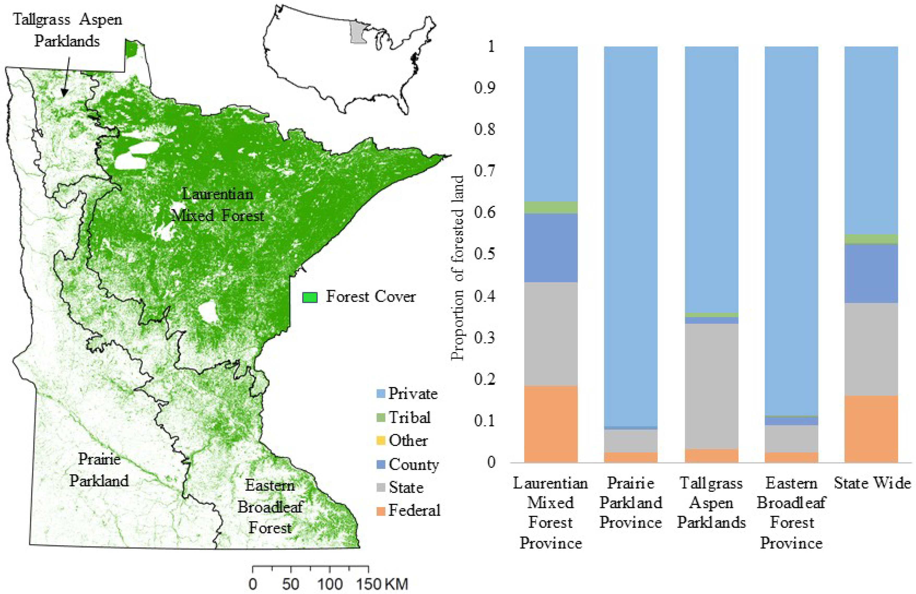
2.1. Study Area

We focused our case study on the forested lands of Minnesota, USA, which encompasses a variety of ownerships that are approximately evenly split between private and public entities (Figure 1). Forests cover approximately 1/3 of the land area in Minnesota and are predominantly located in the northern-northeastern portion of the state (Figure 1). A variety of cover types occur in the region, with aspen—birch (Populus spp.—Betula spp.) and spruce—fir (Picea marianaAbies balsamea) types dominant, and to a lesser extent pine (Pinus resinosa, Pinus strobus, Pinus banksiana), oak (Quercus spp.), and northern hardwoods [27]. Wetlands, including forested bogs, peatlands, and swamps, are found extensively throughout the forested region of the state. A variety of land uses occur in Minnesota forests including timber production, mining operations, and recreation. The four ecological provinces of Minnesota (Figure 1), which are defined by their climate, geologic history, soils, hydrology, and associated vegetation, include: Eastern Broadleaf Forest Province (4.9 million ha); Laurentian Mixed Forest Province (9.3 million ha); Prairie Parkland Province (6.5 million ha); and Tallgrass Aspen Parklands Province (1.2 million ha) [28].
For the purpose of our study, we focused on fast forest change events, which we define as those that occur within three years or less, which result in immediate changes in spectral indices that are often associated with canopy mortality. Several types of fast forest disturbances occur across the Great Lakes states including land use conversion, timber harvest, wildfire, flooding, extreme weather events, in addition to other natural agents that occur somewhat infrequently (e.g., outbreaks of insect defoliators with immediate impacts on spectral indices). While three years may seem like a long duration for characterizing what we are considering “fast” disturbances, after initial exploration of change events in our study region, we identified the prevalence of multi-year harvest and land conversion activities that we wanted to capture, while the three-year threshold tended to exclude the majority of slower declines events which were not the focus of our study. Land use conversion may take the form of transitioning forest to agriculture, urbanization, or the expansion of mining areas. Timber products are a leading industry in Minnesota, and a range of silvicultural techniques are used that influence harvest intensity, treatment area, duration of activity, and post-harvest site preparation management practices. Harvesting occurs on most lands outside the protected Boundary Waters Canoe Wilderness Area and the Voyagers National Park, with the majority occurring on combined public ownerships compared to private lands. Harvest levels increased substantially from 1970–1995, peaking from 1995–2005, and then decreased to a stable level of approximately 2.8–3.0 million cords annually [29], which represents less than 1% of timberland in the state. Wildfires are most common in the northern part of the state, with prescribed burn events more geographically generalized. Large wind blowdown events are also common in the northern Great Lakes Basin region along with other extreme weather events such as less frequent tornados [1]. Flooding may lead to canopy mortality as a result of prolonged inundation of forested wetland areas, impacts of roadways on drainage, and beaver activity.

2.2. Landsat Time Series

We compiled a Landsat time series data set from 1972–2019 to facilitate identification of disturbance events and to aid in the classification of the agent of change. After identifying regional peak growing season characteristics through a sample of annual Normalized Differential Vegetation Index (NDVI) curves, we identified and downloaded Landsat images acquired throughout the growing season from the USGS Earth Explorer website (http://earthexplorer.usgs.gov/) for the years of 1972–2015. Imagery for the years of 2015–2019 were processed within Google Earth Engine (GEE) [30] as a part of later updating efforts described below to develop an efficient work flow for periodic updates of our time series stacks, leveraging recent advances in GEE algorithms and cloud computing. With the high occurrence of clouds in the northern part of the state during the growing season, we attempted to balance the representation of a peak growing season date range with imagery coverage in determining our composite date range, resulting in the time window of 1 July–9 September. We compiled imagery from all Landsat sensors (MSS, TM, ETM+, and OLI) from 1972–2015 across the entire state of Minnesota, encompassing 28 Landsat scenes with a total of 6041 images included in the initial time series stack. To create annual cloud-free composites of spectral indices that were comparable across all sensors, we utilized LandsatLinkr (LLR) [21] in the R programming environment [31], for all pre-processing and cross-sensor harmonization. LLR automates the necessary steps to create annual composites of the spectral tasseled cap indices (brightness, greenness, and wetness) [32] as well as a derivative of greenness and brightness called the tasseled cap angle [33], harmonized throughout the entire span of the Landsat archive, and composited across multiple Landsat scenes. Incorporating multiple images within the annual compositing time window, including images from overlapping scenes where available, we employed the median compositing method for selecting spectral index values for each pixel across the time series. See Vogeler et al. (2018) for additional details on image processing and LLR steps utilized in this study [11].
Following the implementation of LLR to produce harmonized spectral indices across the different Landsat sensors, we employed the IDL-based LandTrendr trend fitting algorithm to smooth year to year spectral noise remaining in the dataset, and to identify spectral trends through time [12]. Fitting trend vertices through Landsat time series data sets is a common approach used to identify areas of change, including both fast events (e.g., fire and harvest) and slower declines (e.g., stress and insects), as well as to characterize recovery trajectories. We employed LandTrendr to fit trends through the composite stacks of each of the tasseled cap indices independently, although the trends for tasseled cap wetness (TCW) were ultimately utilized to identify the timing and change magnitude of the most recent fast disturbance event occurring in a given area. Of the tasseled cap indices, TCW is the most sensitive to changes in forest canopy structure [34]. We utilized Google Earth Engine (GEE) to update the time series through 2019, using comparable pre-processing methods and composite date ranges as those utilized in the processing of the 1972–2015 data base, with the exception of fitting LandTrendr trends to the reduced time frame of 1984–2019 to leverage the available Landsat imagery and LandTrendr algorithm [35] on GEE. The fitted tasseled cap indices for 2015–2019 were then exported from GEE and compiled with the existing 1972–2014 fitted indices time series for the identification of disturbance events and classification of agents. Previous studies have noted increased instability of the first year or two of a Landsat time series data base as these early years lack the benefits of previous years for stabilizing context; similarly, the final year of the time series lacks the context of post-disturbance years [12], which may inflate disturbance areas and cause increased errors in agent classifications. Therefore, we allowed the time series two years to stabilize, and removed both of the ending years in the two time series stacks, 2015 from the initial time series, which was replaced by GEE-based indices and 2019 from the second time series, resulting in a final stabilized time series stack from 1974–2018.
We identified the most recent change events from the time series across the landscape, noting the first year post-change as the year associated with each fast event. Since the focus of this study was to identify patch to stand altering events, where we consider patches as within stand events resulting in large openings in the canopy, we followed the methods of Kennedy et al. (2015) and set a minimum mapping unit of 11 Landsat pixels (slightly more than 1 ha) to determine if a patch was retained in the final change map [15]. The minimum of 11 pixels also serves as a homogeneity check to focus on canopy opening events while excluding smaller spectral change patches, which have a greater probability of being related to spatial misregistration issues.
We used a forest mask to remove non-forest lands to limit change patches to just those occurring within forest. There is potential bias in using a current forest mask to remove non-forest areas in a study that spans four decades because areas that were historically forested but recently converted to non-forest would be missed. To minimize this bias, we created an “if-ever-forest-mask” by stacking annual forest masks from 1973–2018 created by Vogeler et al. (2018) [11] and setting a threshold of three years within a forest class at any point throughout the time series to be considered forest during the study period. While this method reduces the bias of removing stands which may have been converted out of a forest class during the study period, it also represents a liberal classification of “forest” for the current time period and may result in some non-forest change events to be retained in the final product.

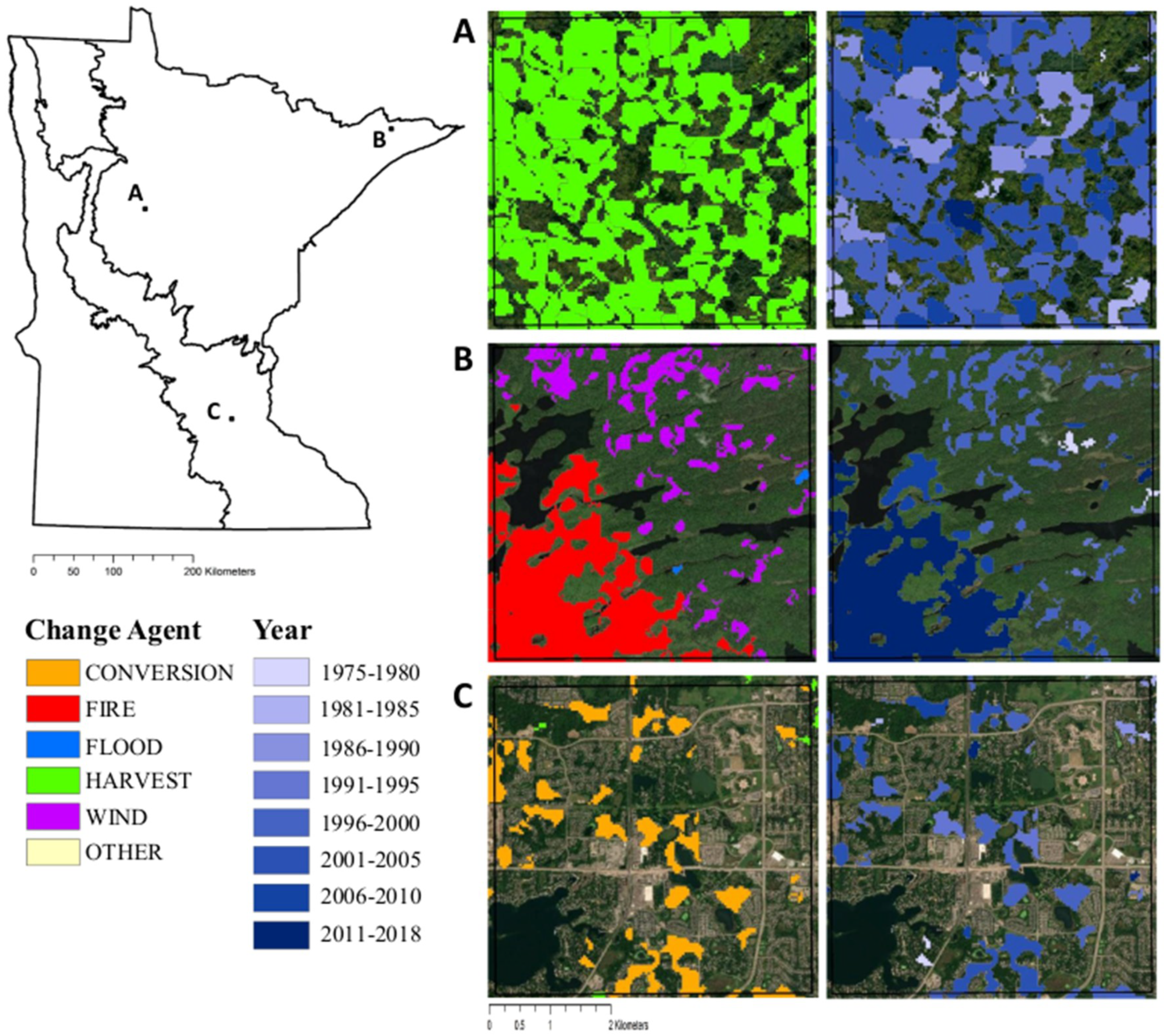
2.3. Change Agent Attribution

Following the identification of the most recent fast change events across the study area, we extracted information about each of the change areas to create a classification model to predict the agent of change for each independent event. Classification predictor variables included: Landsat fitted spectral indices and magnitudes of change, pre- and post-change fitted spectral and canopy cover values, patch area and shape characteristics, topographic indices extracted from Shuttle Radar Topography Mission (SRTM), information about the management protection status as classified by the Gap Analysis Project (GAP) [36] within their Protected Area Data base–US (PAD-US), and key land cover classes related to wetland areas from the 2016 National Land Cover Dataset (NLCD; Table 1) [37]. Canopy cover values were extracted from an annual state-wide data base, also created using Landsat time series methodologies [11]. In addition to basic elevation and slope, we calculated topographic indices representing local hillslope positions and a topographic landform using the Relief Analysis add-on tool [38] for ArcGIS 10.3. Utilizing the GAP PAD-US product [36], we assigned each change patch with a management protection level from 1 to 4 to include as a categorical predictor, with 1 representing the highest level of resource extraction protection such as those found in national parks and wilderness areas, and 4 indicative of areas with no or unknown management protection. As anthropogenic disturbances should be minimal in highly protected areas, our hope was that the inclusion of this categorical variable may help account for these differences in likelihoods of disturbance agents within the levels of land protection.
We compiled a training database of 2747 patches with known agents of change using a combination of historic aerial photos, existing spatial databases (e.g., Monitoring Trends in Burn Severity) [39], and expert knowledge compiled during personal communications with local land managers. Sources of historical aerial imagery included Google Earth Pro for 1990-present, and the database available through the Minnesota Historical Aerial Photographs Online website for pre-1990 aerial photos [40]. All photo interpretations were completed by one trained interpreter familiar with the study area to reduce biases between multiple interpreters. All training patches were classified using a 6-class designation: land conversion out of a forest class (CONVERISON), forest fire (FIRE), flooding related spectral and/or canopy changes (FLOOD), timber harvest (HARVEST), wind and weather-related events (WIND), and other rare or unknown natural events (OTHER). During the identification of training patches, we noted that some identified change events contained standing water related to flood events, which may or may not have led to actual canopy mortality. We included both flooding resulting in spectral changes, as well as events that ended in canopy mortality, within our FLOOD classification, as spatial information about flooding events, whether they result in immediate canopy mortality or not, can be of interest to managers.
We created a random forest classification model [41] using the randomForest R package [42] for the 6-class agent of change designation. After compiling all predictor variables for training patches, we conducted a variable reduction and model selection procedure employing the rfUtilities R package [43]. We then applied the final 6-class model to all unknown patches to predict the agent of change for all most recent fast change events across the study area.

2.4. Change Detection Validation

We followed the methods presented by Olofsson et al. (2014) [44] and Stehman (2014) [45] for the validation of classification maps to quantify area-weighted accuracy measures and confidence intervals for areas of change vs. no-change as well as for each of the change agent classes. We selected a random set of 725 validation map pixels stratified by the six agent classes as well as a seventh class representing areas of forest classified as no-change. We used a combination of the data sources employed in training interpretations (e.g., historic photos) along with plots of the unfitted spectral index trends to aid in the assessment of each of the validation pixels. We assigned a designation of change/no-change and the observed agent of change, which we then compared to the predicted classification to create validation confusion matrices, calculate class and overall accuracies with confidence intervals, and produce an area-weighted coefficient for the estimation of all areas presented in our results.

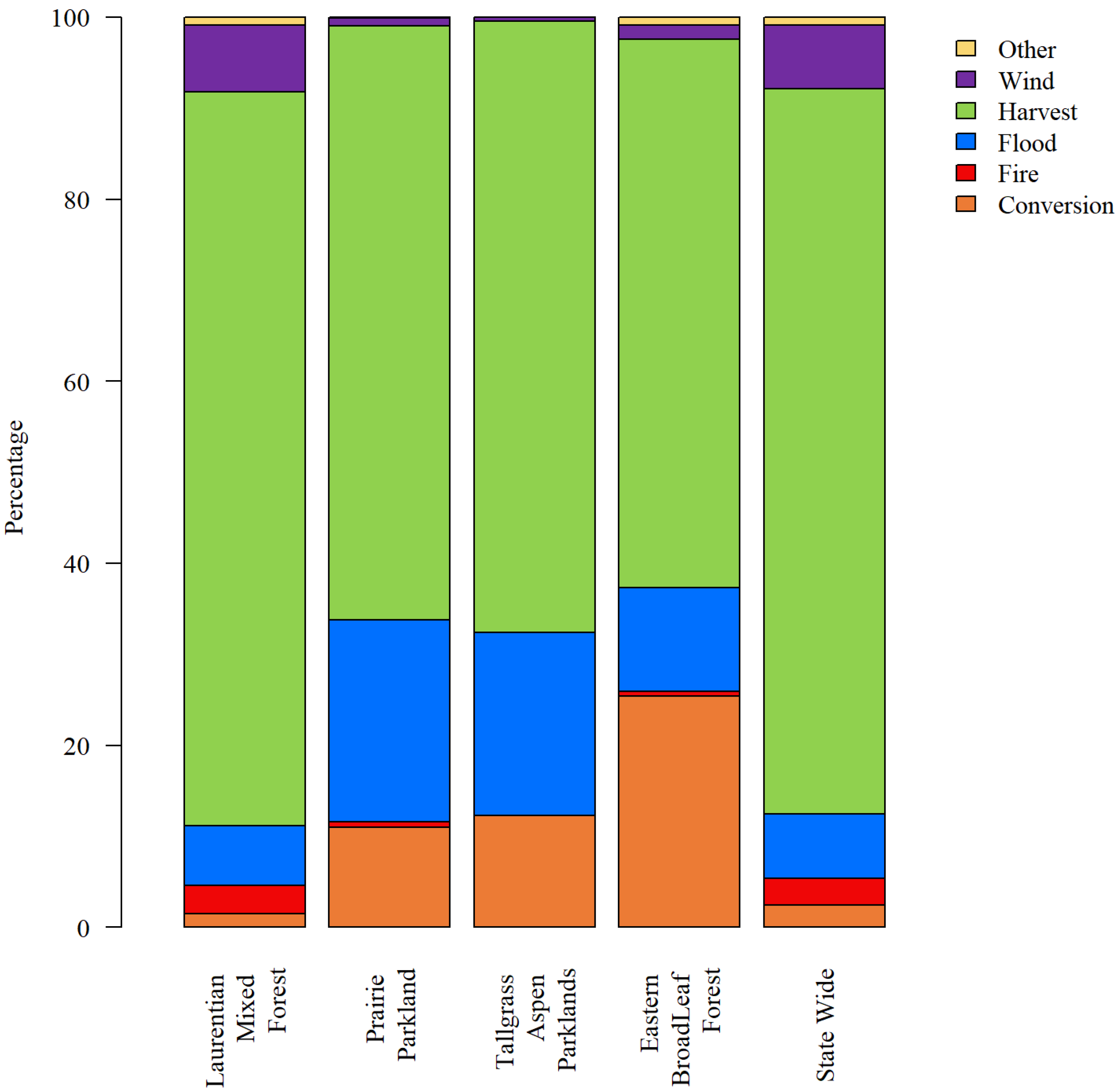
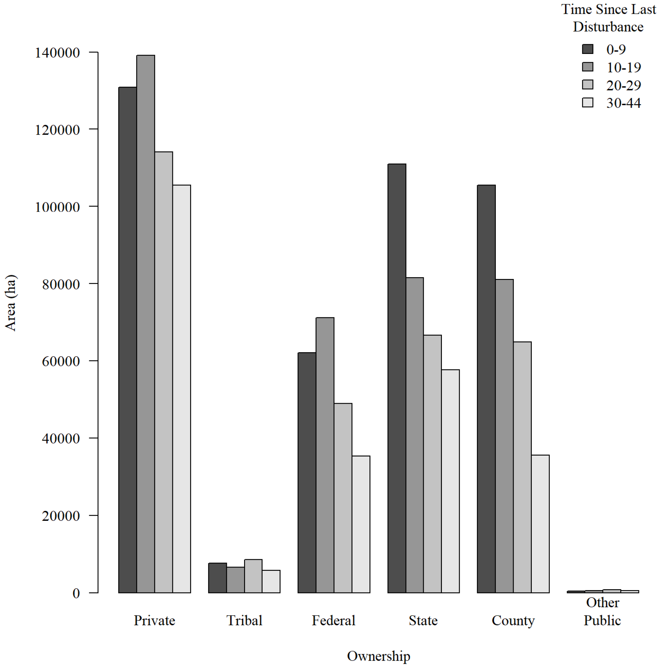
2.5. Spatial and Temporal Summaries

We summarized spatial and temporal trends within forest ownership boundaries as well as within the four ecological regions of Minnesota: eastern broadleaf forest, Laurentian mixed forest, prairie parkland, and tallgrass aspen parkland. We compared the distribution of the different agents of change, magnitudes of agents, as well as time since disturbance classes, across ownerships to identify any spatial or temporal patterns of disturbances within ownerships. Time since last disturbance, along with the magnitude of change, is often related to the succession stage of a stand; thus, in addition to assessing trends in magnitudes of changes by agents, we also utilized the year of onset for each change event to create the following time since disturbance classes with the assumption that they represent different stages of forest succession and associated structures: 0–9 years since disturbance, 10–19 years since disturbance, 20–29 years since disturbance, 30–44 years since disturbance. Leveraging the previously published annual Minnesota canopy cover maps created using the same base Landsat time series spectral data stacks as those used in our study to identify disturbance patterns [11,46], we translated the magnitude of change from each disturbance event into change in percent canopy cover by subtracting the mean pre-disturbance canopy cover from the mean post-disturbance canopy cover, to provide a management-relevant relative measure of magnitudes across agents and ownerships.

3. Results

The Landsat time series methodology utilized in this study was successful in identifying the most recent fast disturbance events across Minnesota from 1974–2018 with a change vs. no-change validation accuracy of 97.2% ± 1.9% (Table 2). The change detection algorithm exhibited higher omission (14.9% ± 9.3%) than commission errors (1.6% ± 1.9%) for the identification of change patches. Omission errors within the validation efforts were often related to the size and intensity of the change event. Change patches close to the minimum size threshold were less likely to be identified, along with patchy natural events where the disturbance impacts were more spread out and barely constituted a contiguous 11 pixels of change. Similarly, lower intensity events also contributed to omission errors, including sivilcultural-thinning activities, which resulted in only minor reductions in canopy. We did not observe any significant differences in error structures of the change and no-change classification if we removed MSS-related change years, supporting its inclusion to extend the time series stack for the identification of fast patch to stand impacting change events.
We further classified disturbance patches by their agents of change (Table 3) with an overall accuracy of 96.5% ± 1.9% (Table 4). Individual disturbance class user and producer errors varied, but all class accuracies were above 78% (Table 4), with HARVEST and CONVERSION exhibiting the highest user accuracies (95.6% ± 3.8% and 92.9% ± 6.2%, respectively) and FIRE and CONVERSION with the highest producer accuracies (98.8% ± 2.4% and 92.6% ± 8.9%, respectively). The lowest user and producer accuracies were observed for the WIND (80.0% ± 9.0%) and HARVEST classes (78.6% ± 10.9%), respectively. Detailed depictions of example patterns of disturbance ages and the classified agents are presented in Figure 2. One of the most prevalent misclassifications were lower intensity harvest patches, such as those that were thinned through strip harvests or localized selective harvests, incorrectly predicted as wind events. There were also some cases where harvests were predicted as flooding and vice versa, which may be due to simultaneous disturbance events (i.e., increase in minor flooding or other moisture related spectral changes immediately following harvest activities) [47] or were a byproduct of post-harvest site-preparation techniques.
During the time period of the study, 17% of forested lands experienced a stand-altering event, although this proportion was calculated using our liberal if-ever-forest-mask, which may bias this estimate through the overestimation of current forested areas; thus, underestimation of proportion of current forested area that experienced a fast change event. Across all regions, harvest was the most prevalent stand replacing causal agent (80% of total disturbed area) followed by wind and flooding, each representing approximately 7% of total disturbance area. Patterns of change agents across the study region show variations in the dominant disturbance events for major stand alterations within the four ecological regions of Minnesota (Figure 3). The Laurentian Mixed Forest ecoregion, which has the largest proportion of public lands including the Chippewa and Superior National Forests, Boundary Waters Canoe Wilderness Area, and Voyagers National Park, had the most variation in agents of change with the highest proportion of area impacted by wind and fire events compared to the other regions (Figure 3). The Laurentian Mixed Forest ecoregion also had the highest proportion of forested land and disturbed area in general (95% of the disturbed forest). The Eastern Broadleaf Forest ecoregion, home to the densely populated metropolitan area of the Twin Cities, has the largest proportion of private ownership in the state and the highest proportion of land conversion across the study time period (Figure 3).
Land ownerships exhibited varying patterns of likelihood of disturbance across the different change agent classes. The highest proportion of most of the natural disturbance classes, including fire and wind, occurred on federal lands (86% of all fire activity and 50% of all wind activity), which includes the protected Boundary Waters Canoe Wilderness Area and the Voyagers National Park. While harvest was the most likely stand altering disturbance agent across all ownerships (Table 5), the majority of harvest activity in terms of actual land area occurred on private and state managed lands encompassing 469,198 ha (38% of all harvest activity) and 311,553 ha (25% of all harvest activity), respectively. It should be noted that the private and state ownership classes also represent the two largest forest land holdings in the state (Figure 1). Land conversions were most likely to occur on private lands (84% of all conversion area).
Assessments of the relative changes in canopy cover within events of different disturbance agents and ownerships revealed significantly higher changes in cover as a result of harvests and land conversions over the other agents, and a tendency for generally higher impacts of events on canopy cover within the “county” ownership class (Figure 4). When we focused on harvest events specifically, the trend for cover magnitudes were similar as those from combined disturbance events, with “county” lands exhibiting significantly higher changes in canopy cover from harvest events (e.g., more clear-cuts) followed by “other public” and “state” managed lands, although harvests within all ownerships spanned a range of sivilcultural techniques and harvest intensities. We acknowledge that the canopy cover maps represent all functional woody vegetation cover over two meters [11], including large woody shrubs common to Minnesota forests, and therefore is not just a measure of canopy removal from the disturbance event, although we believe that it is appropriate as a relative measure of change across the disturbance events. In general, magnitudes of cover changes appeared low, even within canopy clearing events such as clear-cuts, which could be a product of revealed understory trees, a quick release in growth of tall woody understory shrubs, or overestimation of base cover within the annual cover maps. We also calculated change in canopy cover as the mean pre-disturbance cover subtracted from the mean post-disturbance cover within each individual change event; therefore, the resulting change value is impacted by minimal cover change along edges and in areas of retained trees, as well as smoothing over individual pixels within the change patch that may have experienced significantly higher changes in percent cover.
Within the time since disturbance classes assessed in this study (≤44 years since disturbance), the majority of forest lands across all land ownerships fall within the two youngest time since disturbance age bins (0–9 and 10–19 years since disturbance; Figure 5). County and state-owned lands exhibited higher proportions of areas within the youngest time since disturbance class, while the second youngest class represented the highest proportion of area within federal, tribal, and private lands (Figure 5). Due to the small forest area within the “other public” category, we did not further evaluate age class distributions within this ownership. Harvest was the driving agent for all time since disturbance classes, with the largest proportion of harvested area within the second youngest class (10–19 years since disturbance; Figure 6). Fire and conversion were more frequent within the youngest class (0–9 years since disturbance), while wind and the other class exhibited their highest influence within the second youngest time since disturbance class (Figure 6).

4. Discussion

As forest management agencies increasingly engage in all lands management, spatial information about forest age, condition, and disturbance histories across the landscape may provide a valuable tool for cross-ownership planning. Currently in the western USA, all lands management efforts are becoming more common for fuel reduction treatments in the mitigation of wildfire risks and/or restoration efforts to promote forest resilience to fire events [7], where forest structural stage and disturbance history information may aid in project planning. On a more global stage, studies have begun to explore the utility of cross-ownership assessments for greenhouse accounting frameworks requiring spatially explicit information about forest change, specifically anthropogenic management activities and land conversions, to serve as important accounting and monitoring inputs [48]. More specific to Minnesota, a recent report released by the Minnesota Forest Resources Council identified a key research priority for multi-ownership management related to determining relationships between the spatial arrangement of forest conditions (age class structure, cover types, patch size distribution) and forest resources such as fiber availability, water quality, and wildlife habitat, among others [49]. The approach we have presented here directly addresses information needs of all lands management efforts, and our results show promise for statewide assessments of forest structure and change and its influence on forest resources. With contiguous coverage across the state, independent of land ownership, spatial and temporal information about disturbance patterns presented in our study will help fill information gaps for support of collaborative management and restoration efforts across ownership boundaries within Minnesota, as well as providing a methodological framework, which could be applied to produce similar spatial products in other regions.
In our study, we harmonized imagery across all Landsat sensors, including the early MSS years, which are rarely incorporated into recent Landsat time series change detection analyses. This approach allowed us to identify and classify an extra decade of events compared to many of the other change detection studies [2,15,16,50], resulting in the characterization of forest disturbances across the state of Minnesota for a time period spanning forty-four years. While we did not detect any variations in accuracy structures across the time periods of the different Landsat sensors within our study, we acknowledge that there still may be some sources of limitations and biases in the incorporation of the MSS era not reflected in the validation accuracies alone. While the pre-processing and harmonization procedures facilitated by LLR may have helped alleviate difficulties faced by the coarser resolutions, reduced spectral information, and increased geo-registration errors of the MSS data (see Vogeler et al. 2018 for details on MSS processing steps) [11], there was still the need for extensive quality assessments and periodic manual intervention throughout the processing steps to ensure the creation of comparable products to that of the later sensors. These interventions included the identification and removal of individual MSS images, which caused artifacts in initial spectral composites, as well as manual geo-registration efforts for an additional 96 MSS images (L1G products) to fill in spatial and temporal gaps due to limited higher quality level 1 products, for which LLR is set up to ingest, for some years and Landsat scenes [11]. In addition, the black and white historic photographs from the MSS era used for validation often had larger time gaps between images and coarser resolutions than more recent aerial photography archives, resulting in lower confidence calls during validation assessments. This means that there is a chance that there were additional small lower intensity disturbances that were missed in the MSS years of our disturbance mapping that we were unable to be detected from the available reference data during map validation, which would result in slightly inflated MSS era related accuracies. Other constraints in using MSS imagery include (1) limited availability of MSS imagery and methodologies in GEE, requiring more local computing resources and processing times, and (2) limited coverage of MSS imagery (as readily useable level 1 products) in many areas outside of the U.S., which restricts international opportunities to construct longer time series with MSS data.
Previous studies evaluating time series change detection from 1984-forward utilizing various trend fitting algorithms exhibited similar accuracies to our overall change detection accuracy of 97.2% ± 1.9% [16,50]. Nguyen et al. (2018) utilized a similar LandTrendr segmentation change detection methodology to us, but relied on trends across the normalized burn ratio (NBR) index as opposed to our tasseled cap wetness index for change detection [16]. They reported an accuracy of 87.5% for primary change events across four Landsat scenes within the state of Victoria, Australia [16]. Focusing on the entirety of the province Saskatchewan, Canada, Hermosilla et al. (2015) utilized a Landsat time series break-point detection approach with an overall accuracy of 92.2% for identifying forest change events [50]. In our study, we found higher omission than commission errors for detecting areas of forest change (14.9% ± 9.3% and 1.6% ± 1.9%, respectively), with many of the omission errors attributed to either small (e.g., close to the 11-pixel minimum mapping unit) or lower intensity disturbances (e.g., thinning harvests with high levels of retained canopy). While an underestimation of disturbed area is assumed due to higher omission than commission errors, further validation of the size of individual mapped events could be conducted by digitizing disturbance patches using high resolution reference imagery, if such data exist. Managers and other users of disturbance mapping products may benefit from more detailed validation analyses related to sizes of, and sensitivities to, individual events; thus future work should continue to explore the potential bias of change detection approaches for underestimation in sizes of individual change events and methodological sensitivities to various levels of disturbance intensities (e.g., a range of sivilcultural techniques).
Attributing the causal agent or pattern of change has become a common theme in Landsat time series change detection studies [2,15,16,50] and provides valuable information for land managers and for additional ecological assessments of disturbance regimes and impacts on ecological services. Despite variations in disturbance agent and temporal regimes across regions and forest types, we were able to predict causal agents with class accuracies above 78%, with the majority above 90%, and an overall 7-class (six disturbance classes and one non-change class) accuracy of 96.5% ± 1.9% across the diverse forest systems of Minnesota. When relying on spectral trends for change detection and classification of agents, there are some potential limitations of the data to differentiate between disturbance classes when they result in similar post change structures. For example, patches that experienced lower intensity silvicultural practices such as thinning and selection harvests were occasionally misclassified as wind or missed in disturbance detection altogether. Further, we chose to focus our identification of disturbance areas on relatively fast moderate-high magnitude change events; thus, our maps do not reflect areas impacted by forest changes related to slower declines, which may be the product of insects and disease, although these evaluations are also possible through Landsat time series approaches [51].
Forest harvest represented significantly higher mean changes in canopy cover compared to the other disturbance agents, with the highest mean cover changes occurring on “county”, “other public”, and “state” managed forest lands. Land ownership can have large impacts on forest disturbance regimes, including sivilcultural intensities, rotation lengths, fire suppression, and salvage harvesting of natural events. For instance, natural events, including fire and wind, were most likely to occur on federal lands. This may be in part due to the historical disturbance patterns of ecological regions, where the majority of federal lands, as well as historic occurrences of large fire events, occur within the Laurentian Mixed Forest Province of Minnesota. The higher likelihood of the most recent change being a wind or fire event on federal lands may also be attributed to the federally owned Boundary Waters Canoe Wilderness Area and the Voyagers National Park, which are protected from harvest and land conversion activities. While wind and fire activities within this ecoregion of Minnesota may also occur on private, state, and county lands, they also have a higher probability of experiencing salvage logging after the natural disturbance event, which would then be reported as the most recent change event within our disturbance map.
By delineating the agent(s) of forest change, we are able to provide greater insight into the residual forest structures, recovery patterns, and potential impacts on ecosystem services. For example, in some instances fire and wind may result in similar canopy mortality as harvest activities, but that reduction in live biomass is likely retained at some level as standing or downed dead wood as opposed to the reduction in canopy being the result of timber removal during silvicultural practices. Those residual standing or downed dead wood legacies within fire or wind impacted stands may provide valuable habitat resources to a variety of wildlife species [52,53] and contribute to the overall structural diversity of the stand. In addition to providing direct insights into residual structures through the identification of change agents, our methodologies may also aid additional modeling and mapping efforts of more detailed structural patterns and stand boundaries through the fusion of remote sensing data sources [19,20]. Combining the historic Landsat time series products with the structural sensitivity of active remote sensing (e.g., lidar) may assist in characterizing difficult to map forest attributes such as biomass [20] and standing dead wood habitat resources [19], which provides value for carbon accounting [54] and monitoring of wildlife habitat for species of conservation interest [53]. Recovery trajectories may also be impacted by the agent of forest change [2]. A study utilizing Landsat spectral trends to assess short- and long-term recovery patterns following fire and harvest events across Canadian forests found that harvest areas recovered more consistently and quickly than fire impacted forests when normalized for magnitudes of change [2]. Through the identification of the timing, extent, magnitude, and agent of disturbance events, we can provide insight into potential recovery trajectories and aid in further research as to the varying impacts of change agents on residual structures and recovery patterns across different forest systems.

5. Conclusions

As access to affordable remote sensing imagery and cloud computing resources improve, and the temporal records of field and remote sensing-based data bases continue to lengthen, opportunities are increasing to provide spatial records of forest change and recovery patterns across large extents. The findings we presented here demonstrate an approach to quantify most recent fast disturbances over long time periods to provide spatial and temporal information about forest change events and their associated causal agents. These types of data may facilitate cross-ownership monitoring, planning, and restoration efforts to better address the scale of forest ecosystem processes, and improve the efficiency of efforts to address the complicated nature of stressors that forest currently face. The potential of altered disturbance regimes as well as intensities and extents of natural change events with climate change, require drawing on new technologies, management approaches, and large-scale planning efforts to maintain general forest health and functioning across the landscape and the vital ecosystem services that forests provide. The disturbance map presented in this study is freely available on the Minnesota Geospatial Commons (https://gisdata.mn.gov/dataset/env-fast-forest-disturbances).
The unmatched nature of the Landsat archive for providing comparable forest attribute and change information across more than four decades highlights the value of the totality of the Landsat program to the larger geospatial, ecological research, and forest management communities. Our study demonstrates an approach for the harmonization of all Landsat sensors and the identification of change events across the Landsat archive. However, the incorporation of MSS imagery to extend the time series analyses required extensive time and effort, and spatial applicability of our methods are restricted to geographic regions with adequate temporal and spatial coverage of MSS imagery available as terrain corrected level 1 products, which may be limited in some international locations. Further studies should continue to evaluate the values and potential limitations for applications of the extended Landsat time series data set.

Author Contributions

J.C.V. performed the data processing, collected all training and validation data, and wrote the manuscript; J.C.V. and P.A.F. conducted the spatial/temporal trend analyses and summarized the data for the paper; R.A.S. and M.J.F. conceived the original concept, secured funding for the project, and provided insights and feedback throughout the data processing; P.A.F, R.A.S., and M.J.F. reviewed and revised the manuscript. All authors have read and agreed to the published version of the manuscript.

Funding

This research was supported by the Environment and Natural Resources Trust Fund and the Minnesota Department of Natural Resources.

Acknowledgments

We would like to thank Justin Braaten for inviting us to serve as early beta-testers for LandsatLinkr and his assistance in establishing our initial time series compositing methodologies, and Robert Kennedy for access to the LandTrendr algorithm. We would also like to thank Mark Nelson of the USFS Northern Research Station for his regional knowledge and insights throughout the duration of this project.

Conflicts of Interest

The authors declare no conflict of interest.

References

  1. Frelich, L.E. Forest Dynamics and Disturbance Regimes: Studies from Temperate Evergreen-Deciduous Forests; Cambridge University Press: Cambridge, UK, 2002; 266p. [Google Scholar]
  2. White, J.C.; Wulder, M.A.; Hermosilla, T.; Coops, N.C.; Hobart, G.W. A nationwide annual characterization of 25 years of forest disturbance and recovery for Canada using Landsat time series. Remote Sens. Environ. 2017, 194, 303–321. [Google Scholar] [CrossRef]
  3. Jurgensen, M.F.; Harvey, A.E.; Graham, R.T.; Page-Dumroese, D.S.; Tonn, J.R.; Larsen, M.J.; Jain, T.B. Impacts of timber harvesting on soil organic matter, nitrogen, productivity, and health of Inland Northwest forests. For. Sci. 1997, 43, 234–251. [Google Scholar]
  4. Carignan, R.; D’Arcy, P.; Lamontagne, S. Comparative impacts of fire and forest harvesting on water quality in Boreal Shield lakes. Can. J. Fish. Aquat. Sci. 2000, 57, 105–117. [Google Scholar] [CrossRef]
  5. Lindenmayer, D.B.; Noss, R.F. Salvage logging, ecosystem processes, and biodiversity conservation. Conserv. Biol. 2006, 20, 949–958. [Google Scholar] [CrossRef]
  6. Yatskov, M.A.; Harmon, M.E.; Barrett, T.M.; Dobelbower, K.R. Carbon pools and biomass stores in the forests of Coastal Alaska: Uncertainty of estimates and impact of disturbance. For. Ecol. Manag. 2019, 434, 303–317. [Google Scholar] [CrossRef]
  7. Charnley, S.; Kelly, E.C.; Wendel, K.L. All lands approaches to fire management in the Pacific West: A typology. J. For. 2016, 115, 16–25. [Google Scholar] [CrossRef]
  8. USDA. Towards a Shared Stewardship across Landscapes: An Outcome-Based Investment Strategy; FS-1118; USDA: Washington, DC, USA, 2018.
  9. Jacobs, K. Teams at their core: Implementing an “all LANDS approach to conservation” requires focusing on relationships, teamwork process, and communications. Forests 2017, 8, 246. [Google Scholar] [CrossRef] [Green Version]
  10. Cohen, W.; Healey, S.; Yang, Z.; Stehman, S.; Brewer, C.; Brooks, E.; Gorelick, N.; Huang, C.; Hughes, M.; Kennedy, R.; et al. How similar are forest disturbance maps derived from different Landsat time series algorithms? Forests 2017, 8, 98. [Google Scholar] [CrossRef]
  11. Vogeler, J.C.; Braaten, J.D.; Slesak, R.A.; Falkowski, M.J. Extracting the full value of the Landsat archive: Inter-sensor harmonization for the mapping of Minnesota forest canopy cover (1973–2015). Remote Sens. Environ. 2018, 209, 363–374. [Google Scholar] [CrossRef]
  12. Kennedy, R.E.; Yang, Z.; Cohen, W.B. Detecting trends in forest disturbance and recovery using yearly Landsat time series: 1. LandTrendr—Temporal segmentation algorithms. Remote Sens. Environ. 2010, 114, 2897–2910. [Google Scholar] [CrossRef]
  13. Huang, C.; Goward, S.N.; Masek, J.G.; Thomas, N.; Zhu, Z.; Vogelmann, J.E. An automated approach for reconstructing recent forest disturbance history using dense Landsat time series stacks. Remote Sens. Environ. 2010, 114, 183–198. [Google Scholar] [CrossRef]
  14. Zhu, Z.; Woodcock, C.E. Continuous change detection and classification of land cover using all available Landsat data. Remote Sens. Environ. 2014, 144, 152–171. [Google Scholar] [CrossRef] [Green Version]
  15. Kennedy, R.E.; Yang, Z.; Braaten, J.; Copass, C.; Antonova, N.; Jordan, C.; Nelson, P. Attribution of disturbance change agent from Landsat time-series in support of habitat monitoring in the Puget Sound region, USA. Remote Sens. Environ. 2015, 166, 271–285. [Google Scholar] [CrossRef]
  16. Nguyen, T.H.; Jones, S.D.; Soto-Berelov, M.; Haywood, A.; Hislop, S. A spatial and temporal analysis of forest dynamics using Landsat time-series. Remote Sens. Environ. 2018, 217, 461–475. [Google Scholar] [CrossRef]
  17. Pedlar, J.H.; Pearce, J.L.; Venier, L.A.; McKenney, D.W. Coarse woody debris in relation to disturbance and forest type in boreal Canada. For. Ecol. Manag. 2002, 158, 189–194. [Google Scholar] [CrossRef]
  18. Foster, D.R.; Knight, D.H.; Franklin, J.F. Landscape patterns and legacies resulting from large, infrequent forest disturbances. Ecosystems 1998, 1, 497–510. [Google Scholar] [CrossRef]
  19. Vogeler, J.C.; Yang, Z.; Cohen, W.B. Mapping post-fire habitat characteristics through the fusion of remote sensing tools. Remote Sens. Environ. 2016, 173, 294–303. [Google Scholar] [CrossRef]
  20. Pflugmacher, D.; Cohen, W.B.; Kennedy, R.E. Using Landsat-derived disturbance history (1972–2010) to predict current forest structure. Remote Sens. Environ. 2012, 122, 146–165. [Google Scholar] [CrossRef]
  21. Braaten, J.D.; Cohen, W.B.; Yang, Z. LandsatLinkr (Version 0.4.2-beta). Zenodo. 2017. Available online: http://dx.doi.org/10.5281/zenodo.807733 (accessed on 5 September 2019).
  22. Chavez, P.S. Image-based atmospheric corrections-revisited and improved. Photogramm. Eng. Remote Sens. 1996, 62, 1025–1035. [Google Scholar]
  23. Kennedy, R.E.; Cohen, W.B. Automated designation of tie-points for image-to-image coregistration. Int. J. Remote Sens. 2003, 24, 3467–3490. [Google Scholar] [CrossRef] [Green Version]
  24. Braaten, J.D.; Cohen, W.B.; Yang, Z. Automated cloud and cloud shadow identification in Landsat MSS imagery for temperate ecosystems. Remote Sens. Environ. 2015, 169, 128–138. [Google Scholar] [CrossRef] [Green Version]
  25. Savage, S.L.; Lawrence, R.L.; Squires, J.R.; Holbrook, J.D.; Olson, L.E.; Braaten, J.D.; Cohen, W.B. Shifts in forest structure in Northwest Montana from 1972 to 2015 using the landsat archive from multispectral scanner to operational land imager. Forests 2018, 9, 157. [Google Scholar] [CrossRef] [Green Version]
  26. Cohen, W.B.; Spies, T.A.; Alig, R.J.; Oetter, D.R.; Maiersperger, T.K.; Fiorella, M. Characterizing 23 years (1972–95) of stand replacement disturbance in western Oregon forests with Landsat imagery. Ecosystems 2002, 5, 122–137. [Google Scholar] [CrossRef]
  27. Miles, P.D.; VanderSchaaf, C.L. Forests of Minnesota, 2014; Resource Update FS-44; U.S. Department of Agriculture, Forest Service, Northern Research Station: Newtown Square, PA, USA, 2015; 4p.
  28. Minnesota Department of Natural Resources. Ecological Classification System. Available online: https://www.dnr.state.mn.us/ecs/index.html (accessed on 10 August 2019).
  29. Minnesota Department of Natural Resources. Minnesota’s Forest Resources 2017. Available online: http://files.dnr.state.mn.us/forestry/um/forest-resources-report-2017.pdf (accessed on 15 October 2019).
  30. Gorelick, N.; Hancher, M.; Dixon, M.; Ilyushchenko, S.; Thau, D.; Moore, R. Google Earth Engine: Planetary-scale geospatial analysis for everyone. Remote Sens. Environ. 2017, 202, 18–27. [Google Scholar] [CrossRef]
  31. R Core Team. R: A Language and Environment for Statistical Computing; R Foundation for Statistical Computing: Vienna, Austria, 2016; Available online: https://www.R-project.org/ (accessed on 9 July 2019).
  32. Crist, E.P. A TM tasseled cap equivalent transformation for reflectance factor data. Remote Sens. Environ. 1985, 17, 301–306. [Google Scholar] [CrossRef]
  33. Powell, S.L.; Cohen, W.B.; Healey, S.P.; Kennedy, R.E.; Moisen, G.G.; Pierce, K.B.; Ohmann, J.L. Quantification of live aboveground forest biomass dynamics with Landsat time-series and field inventory data: A comparison of empirical modeling approaches. Remote Sens. Environ. 2010, 114, 1053–1068. [Google Scholar] [CrossRef]
  34. Healey, S.P.; Yang, Z.; Cohen, W.B.; Pierce, D.J. Application of two regression-based methods to estimate the effects of partial harvest on forest structure using Landsat data. Remote Sens. Environ. 2006, 101, 115–126. [Google Scholar] [CrossRef]
  35. Kennedy, R.E.; Yang, Z.; Gorelick, N.; Braaten, J.; Cavalcante, L.; Cohen, W.B.; Healey, S. Implementation of the LandTrendr algorithm on google earth engine. Remote Sens. 2018, 10, 691. [Google Scholar] [CrossRef] [Green Version]
  36. USGS Gap Analysis Project. Protected Area Database of the United States by GAP Status. Available online: https://www.sciencebase.gov/catalog/item/56bba50ce4b08d617f657956 (accessed on 5 September 2019).
  37. Yang, L.; Jin, S.; Danielson, P.; Homer, C.; Gass, L.; Bender, S.M.; Case, A.; Costello, C.; Dewitz, J.; Fry, J.; et al. A new generation of the United States National Land Cover Database: Requirements, research priorities, design, and implementation strategies. ISPRS J. Photogramm. Remote Sens. 2018, 146, 108–123. [Google Scholar] [CrossRef]
  38. Miller, B.A.; Schaetzl, R.J. Digital classification of hillslope position. Soil Sci. Soc. Am. J. 2015, 79, 132–145. [Google Scholar] [CrossRef]
  39. Eidenshink, J.; Schwind, B.; Brewer, K.; Zhu, Z.L.; Quayle, B.; Howard, S. A project for monitoring trends in burn severity. Fire Ecol. 2007, 3, 3–21. [Google Scholar] [CrossRef]
  40. University of Minnesota. Minnesota Historical Aerial Photographs Online. Available online: https://apps.lib.umn.edu/mhapo/# (accessed on 19 August 2019).
  41. Breiman, L. Random forests. Mach. Learn. 2001, 45, 5–32. [Google Scholar] [CrossRef] [Green Version]
  42. Liaw, A.; Wiener, M. Classification and regression by randomForest. R News 2002, 2, 18–22. [Google Scholar]
  43. Evans, J.S.; Murphy, M.A. Package “rfUtilities”; Version 2.1-3; R Package: Vienna, Austria, 2015. [Google Scholar]
  44. Olofsson, P.; Foody, G.M.; Herold, M.; Stehman, S.V.; Woodcock, C.E.; Wulder, M.A. Good practices for estimating area and assessing accuracy of land change. Remote Sens. Environ. 2014, 148, 42–57. [Google Scholar] [CrossRef]
  45. Stehman, S.V. Estimating area and map accuracy for stratified random sampling when the strata are different from the map classes. Int. J. Remote Sens. 2014, 35, 4923–4939. [Google Scholar] [CrossRef]
  46. Minnesota Geospatial Commons. Annual Canopy Cover (1973–2018) in Minnesota. Available online: https://gisdata.mn.gov/dataset/env-annual-canopy-cover (accessed on 20 September 2019).
  47. Slesak, R.A.; Lenhart, C.; Brooks, K.; D’Amato, A.W.; Palik, B. Water table response to simulated emerald ash borer mortality and harvesting in black ash wetlands, Minnesota USA. Can. J. For. Res. 2014, 44, 961–968. [Google Scholar] [CrossRef]
  48. Cowie, A.L.; Kirschbaum, M.U.; Ward, M. Options for including all lands in a future greenhouse gas accounting framework. Environ. Sci. Policy 2007, 10, 306–321. [Google Scholar] [CrossRef]
  49. Minnesota Forest Resources Council. Priority Research to Sustain Minnesota’s Forest Resources. Available online: http://mn.gov/frc/docs/FINAL_ACCESSIBLE_RAC%20Report%20A11Y.pdf (accessed on 9 September 2019).
  50. Hermosilla, T.; Wulder, M.A.; White, J.C.; Coops, N.C.; Hobart, G.W. Regional detection, characterization, and attribution of annual forest change from 1984 to 2012 using Landsat-derived time-series metrics. Remote Sens. Environ. 2015, 170, 121–132. [Google Scholar] [CrossRef]
  51. Cohen, W.B.; Yang, Z.; Stehman, S.V.; Schroeder, T.A.; Bell, D.M.; Masek, J.G.; Huang, C.; Meigs, G.W. Forest disturbance across the conterminous United States from 1985–2012: The emerging dominance of forest decline. For. Ecol. Manag. 2016, 360, 242–252. [Google Scholar] [CrossRef]
  52. Nappi, A.; Drapeau, P. Pre-fire forest conditions and fire severity as determinants of the quality of burned forests for deadwood-dependent species: The case of the black-backed woodpecker. Can. J. For. Res. 2011, 41, 994–1003. [Google Scholar] [CrossRef]
  53. Vogeler, J.C.; Yang, Z.; Cohen, W.B. Mapping suitable Lewis’s woodpecker nesting habitat in a post-fire landscape. Northwest Sci. 2016, 90, 421–433. [Google Scholar] [CrossRef]
  54. Hudak, A.T.; Fekety, P.A.; Kane, V.R.; Kennedy, R.E.; Domke, G.M.; Filippelli, S.K.; Falkowksi, M.J.; Smith, A.M.S.; Tinkham, W.T.; Crookston, N.L.; et al. A carbon monitoring system for mapping regional, annual aboveground biomass across the northwestern USA. Environ. Res. Lett. 2020. under review. [Google Scholar]
Figure 1. Land ownerships and forest cover across the ecological provinces of the Minnesota study area.
Forests 11 00362 g001
Figure 2. Example insets of most recent fast disturbances within Minnesota by disturbance agent classifications and time since disturbance classes. Inset (A) falls within a mosaic of public land ownership, (B) is located within the Boundary Waters Canoe Wilderness Area, and (C) is within the twin cities developed area of Minneapolis and St. Paul.
Forests 11 00362 g002
Figure 3. Proportion of area for the period of 1974–2018 by agent classes within Minnesota ecological regions.
Forests 11 00362 g003
Figure 4. Mean patch-level change in canopy cover by (A) agent and (B) ownership for disturbances represented by the Minnesota most recent fast disturbance maps for the period 1974–2018. The error bars represent the 95% confidence interval around the mean. Note: change in canopy cover is calculated as the mean pre-disturbance canopy cover subtracted from the mean post-disturbance canopy cover.
Forests 11 00362 g004
Figure 5. Time since last disturbance class areas summarized by land ownerships.
Forests 11 00362 g005
Figure 6. Time since last disturbance class areas summarized by change agents.
Forests 11 00362 g006
Table 1. Disturbance agent random forest classification model predictors with designations for those retained in the final model following variable reduction procedures. The top three metrics from random forest metric importance rankings are marked with an asterisk.
Metric CategoryMetricMetric DescriptionFinal 6-Class Model
SPECTRALTCB-PrePre-disturbance tasseled-cap brightness
TCG-PrePre-disturbance tasseled-cap greennessX
TCW-PrePre-disturbance tasseled-cap wetnessX
TCA-PrePre-disturbance tasseled-cap angle
TCB-PostPost-disturbance tasseled-cap brightnessX
TCG-PostPost-disturbance tasseled-cap greennessX
TCW-PostPost-disturbance tasseled-cap wetnessX
TCA-PostPost-disturbance tasseled-cap angle
TCB-MagTCB magnitude of changeX
TCG-MagTCG magnitude of changeX
TCW-MagTCW magnitude of changeX
TCA-MagTCA magnitude of change
TCB-RecTCB post event recovery magnitude
TCG-RecTCG post event recovery magnitude
TCW-RecTCW post event recovery magnitude
TCA-RecTCA post event recovery magnitude
TCB-CurTCB current value
TCG-Cur *TCG current valueX
TCW-CurTCW current valueX
TCA-CurTCA current valueX
CANOPY COVERCover-Pre *Pre-disturbance canopy coverX
Cover-PostPost-disturbance canopy coverX
Cover-Mag *Difference between Cover-Post and Cover-PreX
Cover-CurCurrent canopy coverX
PATCH CHARACTERISTICSAreaArea of the disturbance patch (m2)
PerimeterPerimeter of the disturbance patch (m)
AP-RatioRatio of perimeter to area X
TOPOGRAPHICElevationMean elevation X
Hillslope-250 mHillslope position index 250 m radii
Hillslope-500 mHillslope position index 500 m radiiX
LandscapeLandscape position index
MANAGEMENT STATUSPAD-USPAD-US protection classification (1–4)X
LANDCOVER CLASSESWetProportion patch within National Land Cover Dataset (NLCD) classes: open water + emergent herbaceous wetlandsX
Wet-AllProportion patch within NLCD classes: open water + emergent herbaceous wetlands + woody wetlandsX
Table 2. Error matrix of estimated proportions of area for change detection assessment and accuracy estimates from independent validation of 725 pixels of the Minnesota disturbance map for the period 1974–2018. Accuracy uncertainty was calculated as 95% confidence intervals and is reported in parenthesis.
Error MatrixAccuracy
Non-DisturbedDisturbedUser’sProducer’sOverall
Non-Disturbed0.8270.02597.0 (2.2)99.7 (0.3)97.2 (1.9)
Disturbed0.0020.14598.4 (1.9)85.1 (9.3)
Table 3. The error matrix for disturbance class attribution populated by estimated proportions of area for the Minnesota disturbance map for the period 1974–2018.
Observed
Non-DisturbedConversionFireFloodHarvestWindOther
PredictedNon-Disturbed0.8270000.02500
CONVERSION00.004<0.001<0.001<0.00100
FIRE0<0.0010.0050<0.001<0.0010
FLOOD<0.001<0.00100.0110.0010<0.001
HARVEST0.002000.0010.1070.0020
WIND<0.0010000.0020.0100
OTHER<0.001000<0.00100.001
Table 4. Accuracy assessment results for non-disturbed forest and attributed disturbance classes for the Minnesota most recent fast disturbance map (1974–2018). Accuracy uncertainty was calculated as 95% confidence intervals and is reported in parenthesis.
Accuracy
User’sProducer’sOverall
Non-Disturbed97.0 (2.2)99.7 (0.3)96.5 (1.9)
CONVERSION92.9 (6.2)92.6 (8.9)
FIRE90.2 (6.6)98.8 (2.4)
FLOOD89.7 (7.4)91.3 (15.0)
HARVEST95.6 (3.8)78.6 (10.9)
WIND80.0 (9.0)83.1 (19.2)
OTHER89.6 (7.0)87.5 (21.8)
Table 5. Percent of area by agent classes within Minnesota land ownership categories. Numbers in bold identifies the most prevalent disturbance agent for each ownership category.
Percent of Disturbance Agents by OwnershipPercent of Total Disturbed Forest
ConversionFireFloodHarvestWindOther
State0.570.869.1783.615.040.7525.19
Federal0.2516.875.1552.7223.461.549.96
Private5.720.447.2182.103.810.7137.93
Tribal1.510.0611.3783.203.520.342.24
County0.680.245.6889.163.500.7324.51
Other Public10.950.365.5979.683.270.150.17
State Wide2.482.947.0279.717.020.84

