Article

Mapping Forest Disturbances between 1987–2016 Using All Available Time Series Landsat TM/ETM+ Imagery: Developing a Reliable Methodology for Georgia, United States

Warnell School of Forestry and Natural Resources, University of Georgia, 180 E Green Street Athens, GA 30602, USA
*
Author to whom correspondence should be addressed.
Forests 2020, 11(3), 335; https://doi.org/10.3390/f11030335
Submission received: 15 February 2020 / Revised: 12 March 2020 / Accepted: 14 March 2020 / Published: 17 March 2020
(This article belongs to the Section Forest Inventory, Modeling and Remote Sensing)

Abstract

:
Forest resources have a high economic value in the State of Georgia (USA) and the landscape is frequently disturbed as a part of forest management activities, such as plantation forest management activities. Thus, tracking the stand-clearing disturbance history in a spatially referenced manner might be pivotal in discussions of forest resource sustainability within the State. The two major objectives of this research are (i) to develop and test a reliable methodology for statewide tracking of forest disturbances in Georgia, (ii) to consider and discuss the use and implications of the information derived from the forest disturbance map. Two primary disturbance detection methods, a threshold algorithm and a statistical boundary method, were combined to develop a robust estimation of recent forest disturbance history. The developed model was used to create a forest disturbance record for the years 1987–2016, through the use of all available Landsat Thematic Mapper (TM)/Enhanced Thematic Mapper (ETM+) data. The final product was a raster database, where each pixel was assigned a value corresponding to the last disturbance year. The overall accuracy of the forest disturbance map was 87%, and it indicated that 4,503,253 ha, equivalent to 29.2% of the total land area in Georgia, experienced disturbances between 1987 and 2016. The estimated disturbed area in each year was highly variable and ranged between 84,651 ha (±36,354 ha) to 211,780 ha (±49,504 ha). By combining the use of the disturbance map along with the 2016 database from the National Land Cover Database (NLCD), we also analyzed the regional variation in the disturbance history. This analysis indicated that disturbed forests in urban areas were more likely to be converted to other land-uses. The forest disturbance record created in this research provides the necessary spatial data and address forest resource sustainability in Georgia. Additionally, the methodology used has application in the analysis of other resources, such as the estimation of the aboveground forest biomass.

1. Introduction

As forest disturbances are a primary factor in the dynamics of a forest ecosystem, the history of disturbances helps keeps track of the condition and development of a forest [1]. Forest disturbances may affect the forest species composition and stand structure depending on the disturbance agent, magnitude, and other complex factors such as soil type, water and nutrient availability, and ecosystem biodiversity [2]. The spatio-temporal patterns of land disturbances are changing due to both anthropogenic and natural agents of disturbance [3]. Hurricanes are a major contributor to deforestation in states bordering the Atlantic and Gulf of Mexico regions of the southern United States [4,5], while in the western United States, forest fires, which are the second largest cause of disturbances, have increased since the mid-1980s [6,7]. In Europe, disturbances caused by wind, bark beetles, and wildfires have also increased over the last century [8]. Mechanical disturbances caused by human activity are another cause of forest disturbance. In Southeast Asia, for instance, demand for monoculture plantations, such as natural rubber, is the main driver of the disturbance of tropical forests [9]. As spatially referenced forest disturbance tracking provides fundamental information in describing the current state of a forest, accurate knowledge of it consequently facilitates the accurate prediction of future conditions and outcomes.
In the southeastern United States, timber harvesting is estimated to be the dominant contributor to forest disturbances [10]. This region encompasses 36% of the timberland, or forested area capable of timber harvest, in the United States [11]. Among the states in the southeastern United States, Georgia has the largest area of timberland. The plantations in Georgia consist predominantly of loblolly pine (Pinus taeda L.), which is the dominant commercial tree species in the southeastern United States. Silvicultural prescriptions for intensively managed plantations include site preparation, herbicide control, fertilization, thinning, and the use of genetically improved seedlings [12]. The continuous efforts to increase plantation volume yields [13,14] have led to the shortening of pine plantation rotations to 20–25 years. Unlike other states having forest practice laws (e.g., Oregon and California) [15], Georgia employs voluntary best management practices (BMPs) to guide forest management activities [16]. While the BMP guidelines include adherence to the federal Clean Water Act, forest owners in Georgia do not have to adhere to a specific scheme of forest practices. Thus, timber plantation managers have considerable flexibility in optimizing their forest management objectives and economic returns, such as intensive forest management and silviculture efforts. Because of the warm and humid climate, the characteristics of the forestland, and common forest management practices, the forest landscape in Georgia evolves rapidly, showing significant changes over relatively short periods of time. The pertinent question regarding the welfare of Georgia forests is whether they are managed on a sustainable basis [17,18]. To assess the sustainability of Georgia forests, it is essential to detect stand-level disturbances, such as final harvests, because knowledge of the date of forest regeneration helps predict the growth and yield of plantations. To this end, spatiotemporal data providing information leading to the identification of the disturbances in a spatially referenced manner can help inform these analyses [15]. It is noteworthy that the Global Forest Change (GFC) dataset provides forest gain and loss with 30-m resolution, globally [19]. However, as the GFC dataset provides the disturbance history starting only after the year 2000, it was necessary to develop our own model to detect the disturbances occurring from the 1980s onward. Although some research has been dedicated to partially tracking the forest disturbance history in Georgia [20,21,22], with the exception of the GFC, no research has covered the disturbance history of the entire state of Georgia.
The Landsat program is the most common source of data for broad-scale forest disturbance analyses because (i) it has a long history starting from 1972, and (ii) its products provide moderate spatial resolution for forest disturbance analyses [23]. Since October 2008, Landsat data managed by the United States Geological Survey (USGS) has been freely available due to a change in the data policy of the Landsat program [24,25,26]. By 2016, more than 3.2 million Landsat images were freely available through the USGS Earth Resources Observation and Science Center archive [27]. This policy change has stimulated new research efforts, such as those aimed at the development of algorithms to detect the land-use change over time. One of the achievements within this research field involved the assessment of forest disturbance trends of the conterminous United States between 1985–2010 [28]. Another example of development within this field is that the emergence of the LandTrendr algorithm, a univariate approach that segments an imagery time series into a series of trends, including changes in forest conditions [9,29].
The Vegetation Change Tracker (VCT) algorithm is another process that has been developed to reconstruct past forest disturbance history from a series of Landsat imagery. With this algorithm, changes in the spectral-temporal properties of vegetation over time are tracked to detect forest disturbances [22,30]. The index used to detect the change is the Integrated Forest z-score (IFZ), which is computed for each pixel in a Landsat scene. As the VCT can be implemented in a reasonable amount of computational time, and since it does not require extensive parameter tuning, its application toward various topics has been made. Zhu [31] categorizes the VCT algorithm as a thresholding method that detects the change in the land-use, where large enough deviations from the assumed threshold are observed. The advantage of a thresholding method is that its implementation process is more straightforward than other change detection methods, and thus it is possible to implement this method using only one satellite image per year. The disadvantage of a thresholding method is that the performance of the model is profoundly affected by the assumed threshold values. Statistical boundary methods are another group of change detection models that assume time-series spectral values fit within a statistical boundary [32,33,34]. These models detect a change in forest character when any departure from the assumed statistical boundary is observed. This method has been used to detect changes from all available satellite imagery [26] and seems less affected by the seasonality of the data, as the raw time-series satellite data values are subjected to applied statistical procedures, in which the seasonal variation and the noise of the raw data are removed from the transformed values. The difficulty of performing geospatial analysis using all available time-series satellite imagery involves basic information technology management and access to high-performance computing. Google Earth Engine (GEE) [35] has recently made it possible to overcome these two obstacles. GEE is a cloud-based platform that provides the high-performance computing resources necessary to process large-scale satellite imagery without storing and managing the data locally. Recent research has involved using all available time-series Landsat imagery with the GEE platform to assess land-uses, agricultural trends, and forest vegetation [36,37,38].
We hypothesize that the known adversarial effect of thresholding methods can be reduced when combined with statistical boundary methods, through the GEE platform. In addition, it is expected that the disturbance detection map created from the forest disturbance detection model will help us to understand the temporal trajectory of each forest stand. Considering these two aspects of our research background, we set forth two major objectives of this research: first, to develop and test a reliable methodology for statewide tracking of forest disturbances in Georgia; second, to consider and discuss the use and implications of the information derived from the forest disturbance map.

2. Materials and Methods

2.1. Study Area

The study area encompasses the entire state of Georgia (Figure 1). The land area of Georgia totals about 154,000 km2 and contains approximately 100,000 km2 of forests, covering almost 65% of the total land area [39]. Timberland potentially available for commercial use constitutes 97% of the forested area, which is more than any other state. Eighty-nine percent of timberland in Georgia is owned by private landowners or corporate entities [11]. The state is divided into seven ecoregions using the level III classification of the United States Geological Survey [40]. The Southern Coastal Plain ecoregion is the southernmost region of the state and consists of flat plains and low elevations. The primary forest types in the Southern Coastal Plain ecoregion are loblolly pine and slash pine (Pinus elliottii Engelm.), and oak-gum-cypress forests typical of some upland areas and most lowland (wet) areas. The Southeastern Plains ecoregion consists of a mosaic of cropland, pasture, woodland, and forest. Elevations and slopes in the Southeastern Plains ecoregion are greater in magnitude than those found in the Southern Coastal Plain. Oak-hickory-pine and southern mixed forests are two of the predominant species in the Southeastern Plains ecoregion, although there are many pine plantations as well. The Piedmont ecoregion is a transitional area between the Appalachian Mountains and the flat Southeastern Plains. Piedmont includes the Atlanta metropolitan area, where about 57% of the population of Georgia resides [41]; thus, urban areas comprise the most significant portion of the land-use in this ecoregion. The other ecoregions, namely the Blue Ridge, Ridge and Valley, Southwestern Appalachians, and the Interior Plateau, contain parts of the Appalachian Mountains [42]. Among the various ecoregions, intensively managed plantation forests are located predominantly in the Southern Coastal Plain. The ecoregions correspond closely to four major geologic zones of the state: (a) Coastal Plain, (b) Piedmont, (c) Blue Ridge, and (d) Appalachian Plateau. The boundary between the Coastal Plain and the Piedmont (the fall line), running east–west through the middle of Georgia, represents a distinct change in the geological conditions relative to those found in flatter areas containing relatively sandy soils (the Coastal Plain), and those containing rolling hills, with soils derived from the process of metamorphism (the Piedmont, Blue Ridge, and Appalachian Plateau).

2.2. Materials and Methods

Level-1 Precision and Terrain (L1TP) corrected Landsat 5 TM and 7 ETM+ images for all Georgia scenes (Figure 1) acquired between April 1984 and December 2016 were queried in the Google Earth Engine platform. The L1TP satisfies both radiometric and geometric criteria set by USGS [43]. We did not use the Landsat 8 OLI data because upon initial inspection, using Landsat 5, 7, and 8 altogether produced inconsistencies in the surface reflectance value. For each image in each scene, clouds, the cloud shadows, water, and snow were masked out using the C Function of the Mask (CFMask) algorithm [44,45,46]. We filtered out imagery containing a high cloud cover percentage, which is likely to contain cirrus clouds frequently left unmasked by CFMask. After visually inspecting the imagery, we determined not to use imagery obfuscated by more than 50% cloud cover. Landsat 7 acquired after 31 May 2003, is provided as Scan Line Corrector-off imagery. We masked out the blank spaces in the imagery provided by GEE. As a result of the preprocessing, 373 to 453 images per scene were available for further analysis, as summarized in Table 1. In total, 5614 images were deployed in the analysis. On average, the mean cloud cover was 14.5% and the length of the time between images averaged 28.0 days.
To detect forest disturbances, we computed the IFZ for each pixel of each scene based on the methodology applied in the VCT algorithm [22,30]. The IFZ is a vegetation index that represents the normalized distance between a pixel value of multi-spectral satellite imagery and the value of a previously identified reference forest pixel. A small IFZ value for a given period and pixel implies that the pixel describes a relatively stable mature forest, while a large IFZ value indicates a non-forested area. An identified forest region is a group of pixels that represent forested areas and are used as reference pixels for the IFZ calculation. Thirty identified forest regions were selected from the entire state. Fifteen of these regions were selected from deciduous forests, while the rest of the regions were selected from coniferous forests. Each region encompassed approximately 50 ha. The mean and standard deviation of the area was computed from a single image that met the following conditions, (i) was taken between April 1, 2018, and August 31, 2018 and (ii) cloud cover percentage is less than 1%. Huang et al. [22] argue that each Landsat 7 Enhanced Thematic Mapper (ETM+) band has a different sensitivity to forest disturbance. The near-infrared band has low sensitivity, as most of the Near Infrared electromagnetic energy is reflected by land surface type. The red band, Short-wave Infrared (SWIR) 1 band, and SWIR 2 band of the imagery were left for IFZ calculation after removing the bands insensitive to forest disturbance. The IFZ was computed for all of the pixels in all of the images queried.
We set four conditions related to the time-series change in the IFZ to detect a forest disturbance. Only if the time series IFZ meets all four conditions is a disturbance detected. The first of the aforementioned conditions concerns the backward moving average. In the notation below (Equation (1)), t i denotes the date in which the i th scene was taken. The t i is then converted from the standard date format to a decimal value. The integer part corresponds to the year, while the fractional part represents the Julian date in the year.
{ t i R | t 1 , t 2 ,   ,   t n } .
For the i th imagery, x ( t i ) is the i th imagery captured on t i . The set of the imagery selected for t i is denoted as X i ,
X i : { x ( t i 3 ) , x ( t i + 1 3 ) , x ( t i + 2 3 ) , , x ( t i ) }   i .
Let C ( X i ) be the number of elements of X i . Then, the backward moving average of the IFZ for j th pixel in the interval of [ t i 3 , t i ] , denoted as B M A t i j , is formulated as follows:
B M A t i j = k X i F k j C ( X i ) .
The first condition is formulated as follows:
B M A t i j 3 .
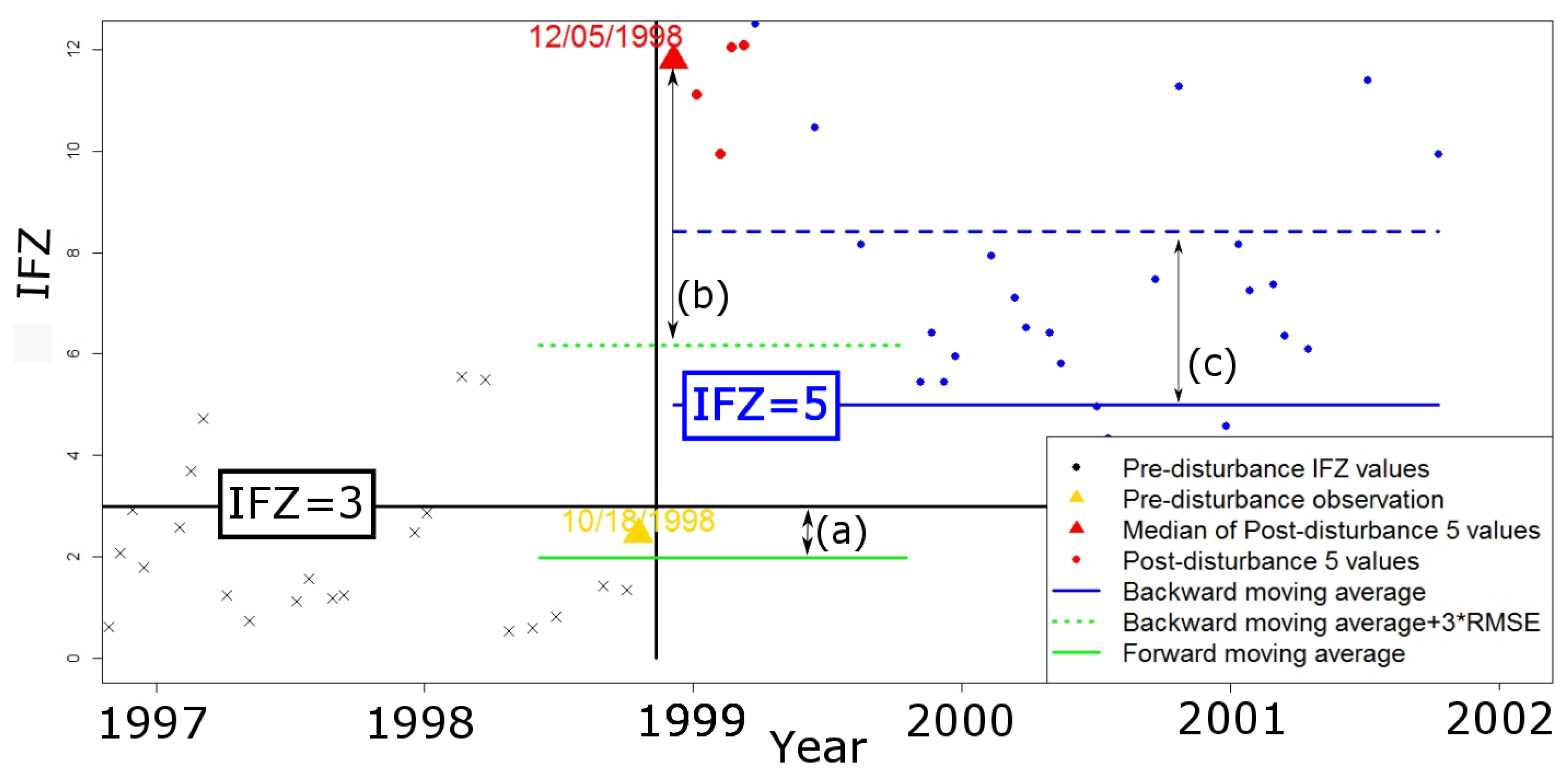
This condition is equivalent to (a) in Figure 2, where the backward moving average has to be higher than 3 for a forest disturbance to be detected. The figure shows that the mean of the last three years of the IFZ values is smaller than 3, although some values are higher than 3.
The second condition is related to the magnitude of change in IFZ value between the pre-disturbance and post-disturbance states. As is argued in [23,37,47], the raw band value and vegetation index following a forest disturbance can deviate from the model’s predicted range. Therefore, we set a condition that detects the presence of the IFZ’s deviation from the past trend, which is quantified by the backward moving average. We assumed that the IFZ values do not continuously deviate from a certain range unless a disturbance occurred. The range was set to the backward moving average plus three times the standard deviation in the last three years of the observations. The standard deviation of the IFZ for the jth pixel is computed as,
S D t i j = k X i ( Z k j B M A t i j ) 2 C ( X i ) .
As the sample of the IFZ values after t(i), the medians of the five successive values after t(i) were selected. The second condition is formulated as follows:
B M A t i j + 3 S D t i j m e d i a n ( Y i ) ,
where Y i : { x ( t i + 1 ) , x ( t i + 2 ) , x ( t i + 3 ) , x ( t i + 4 ) , x ( t i + 5 ) } .
This condition is shown as (b) in Figure 2, where the backward moving average plus three times the standard deviation has to be greater than the median for a forest disturbance to be detected.
The third condition is related to the moving average of the post-disturbance phase. This includes the same computations as those seen in the computation of the backward moving average. The collection of the imagery taken in [ t i + 1 , t i + 3 ] is denoted as Z i .
Z i : { x ( t i + 1 ) , x ( t i + 2 ) , x ( t i + 3 ) , , x ( t i + 3 ) } i .
The forward-moving average is computed as follows:
F M A t i j = k Z i F k j C ( Z i ) .
The third condition requires that,
F M A t i j > 5 .
The third condition is presented as (c) in Figure 2, where the forward-moving average has to be greater than 5 for a forest disturbance to be detected. As the fourth and final condition of the disturbance, the magnitude of the disturbance was computed. The magnitude is the average distance of the post-disturbance IFZ values from the threshold IFZ value. We used IFZ = 3 as the threshold value; it is equivalent to the root mean square difference of the post-disturbance IFZ values from the threshold.
All of the conditions were computed for each pixel in each image. The disturbance detection model iteratively applied the four conditions from the oldest image to the most recent image. If the model detects a disturbance for a given pixel in an image, the Julian date was assigned to the disturbance map raster. Otherwise, nothing is assigned to the pixel. Although a specific date when a disturbance was detected was recorded to the disturbance map raster, only the year was retained, since our interest lies only in the annual disturbances. After running the algorithm forward in time toward the most recent image, a single layer raster, of which pixels represent the last disturbance year, was created. The pixels without any disturbance record were assigned a non-disturbance value.

2.3. Post-Processing

We conducted a post-processing effort after developing the raw disturbance map. The first task in the post-processing effort was the reduction of “salt and pepper” in the disturbance map. The “salt and pepper” phenomenon refers to scattered pixels that deviate considerably from their neighbors based on the last disturbance year. We removed small clusters of these that were less than nine pixels in size (equivalent to 0.81 ha), considering them to be noise inherent in the data. We adopted from the USDA Forest Inventory and Analysis (FIA) program a definition of the minimum size of disturbance to be 0.404 ha (1 acre). Another post-processing task was to cut the pixels at the edge of each image. The edge of the raw disturbance map had a band of areas that recorded disturbances more frequently than the rest of the area of the map. As a result of visual inspection, it was inferred that the individual images within the Landsat time series stack did not have precisely the same geographic extent. Therefore, the edge pixels were frequently located out of the extent of the imagery and subsequently assigned NA value. Next, we calculated the ratio of Clear Pixels (rCP) for each pixel to determine the pixels that were available in smaller quantities (due to clouds, etc.), within the available imagery across the time horizon. For every pixel in a scene, rCP was calculated as the number of the non-NA pixel values throughout the time series divided by the total number of images available within a scene. It was also determined that some of the pixels that were in specific land-uses, such as rivers, ponds, or buildings, had smaller rCP values than the rest of the pixels. Based on visual inspection, we set rCP = 0.6 as the threshold value for this post-processing effort. Pixels were masked from the forest disturbance map if a pixel had an rCP smaller than the threshold.

2.4. Accuracy Assessment

To validate the forest disturbance map, we established 30 points for each of the 30 disturbance year classes, and 2000 points for the undisturbed classes, using a stratified sampling method. The ratio of points between each disturbance year class and the undisturbed class was equivalent to the initial result of the disturbance detection map, which classified about 70% of the pixels to the undisturbed class. The last disturbance year was visually inspected for each point. Google Earth Pro Historical Imagery (GEPHI), custom GEE API, and the time series Landsat surface Reflectance value chart were used as the data sources. GEPHI selected the imagery used based on the user’s zoom level on the display. When a user magnifies the scale (zooms in), it provides high-resolution imagery, such as QuickBird or NAIP. When the scale is decreased (when the user zooms out), it provides intermediate resolution imagery, such as Landsat. In our inspection, we determined that the combination of Landsat imagery and middle-to-low scale imagery levels was not sufficient to verify the occurrence of a disturbance on a sample point. Therefore, when GEPHI provided only Landsat or Sentinel imagery for a given year, we switched to using a custom GEE API. The custom GEE API showed an annual Landsat mosaic imagery during the growing season for each year from 1984–2018. Although the spatial resolution of the API is 30-ms for all of the mosaics, visual verification of disturbance was possible by increasing the scale (zooming in to the points). For the detection of disturbances before 2005, the custom GEE API was used as the primary data source, as GEPHI did not provide annual high-resolution imagery. A time-series chart of surface reflectance values was generated using the custom GEE API. Although the occurrence of disturbances was not determined solely from the time series chart, the chart was used to ascertain the time range within which disturbances were likely to occur. Of the 2900 points created through the stratified sampling method, we first filtered out 187 points that were located on the boundary of two different stands. This was performed because it is visually difficult to determine the disturbance year for these points. The last disturbance year was detected for the rest of the points by using the aforementioned approach. We created a confusion matrix based on the sample counts and a normal confusion matrix in terms of estimated area proportions [48,49]. The area-based confusion matrix was then used to develop an unbiased estimator of the total area for each disturbance class, with 95% confidence intervals. In addition, overall and producer’s accuracies were calculated using the estimated area proportions for each class in the area-based confusion matrix.
Pixels without a disturbance record in our model were assigned to the undisturbed class. To further classify the undisturbed classes into either persistent forest, persistent non-forest, or into a non-forest-to-forest class, the National Land Cover Database 2016 (NLCD 2016, [50]) was consulted. The NLCD 2016 was developed to create a consistent multitemporal land cover and land cover change map for the conterminous United States, at 30-m spatial resolution, from 2001 to 2016. In the NLCD 2016, deciduous forests, evergreen forests, mixed forests, and woody wetland classes were assigned as the applicable vegetative land-uses. Yang et al. [50] studied the accuracy of a map created from a model of the Appalachian Mountains in the northern part of Georgia (WRS-2 path 18, row 35), and determined that the overall agreement between map and reference labels was 88%. However, the user’s accuracies of evergreen forest, mixed forest, and woody wetland were relatively low (between 32%–62%). The NLCD 2016 raster data was acquired from the Multi-Resolution Land Characteristics Consortium website [51]. For the sake of our goal, reclassification of the original data was performed. The four aforementioned vegetation classes were aggregated into one forest class, while the remaining of the classes were redefined as non-forested. The temporal trajectory of all the land in the state in terms of the forest class was then examined (Table 2). The pixels assigned to the persistent forest class were those with undetected forest disturbances over our time horizon forest disturbance, and were considered as forest in the reclassified NLCD 2016. The persistent non-forest class was assigned to pixels with undetected forest disturbances, which were considered as non-forest in the reclassified NLCD 2016. The disturbed forest class was assigned to pixels with detected forest disturbance within our time horizon, which were also considered as forest in the reclassified NLCD 2016. Pixels with undetected forest disturbances were assigned to the persistent non-forest class and were considered as non-forest in the reclassified NLCD 2016. The disturbed forest class was assigned to pixels with detected forest disturbances within our time horizon, and which were also considered as forest in the reclassified NLCD 2016. It was observed that many pixels with a recent disturbance record were classified as the disturbed non-forest class. Classifying a newly disturbed pixel as non-forest, as of 2016, was appropriate if the forest represented by the pixel had not yet recovered. However, these pixels are more likely to be regenerated as a forest than those pixels within the non-forest areas that were disturbed more than five years ago. Therefore, we categorized the deforested class and recent disturbance class as subclasses of the disturbed non-forest class to examine how much area was left as non-forest for a substantial length of time. In the typical plantation forest management scheme in the southeastern United States, forest regeneration is initiated soon after a major disturbance, such as a final harvest or a fire. Thus, we classified pixels within the disturbed non-forest class detected as being disturbed after 2011 into the recent disturbance subclass, while the rest of the pixels, belonging to the disturbed non-forest class, were classified as a deforested subclass. As a result, 5 class categories were developed to describe the temporal trajectory of all the land in the state.

3. Results

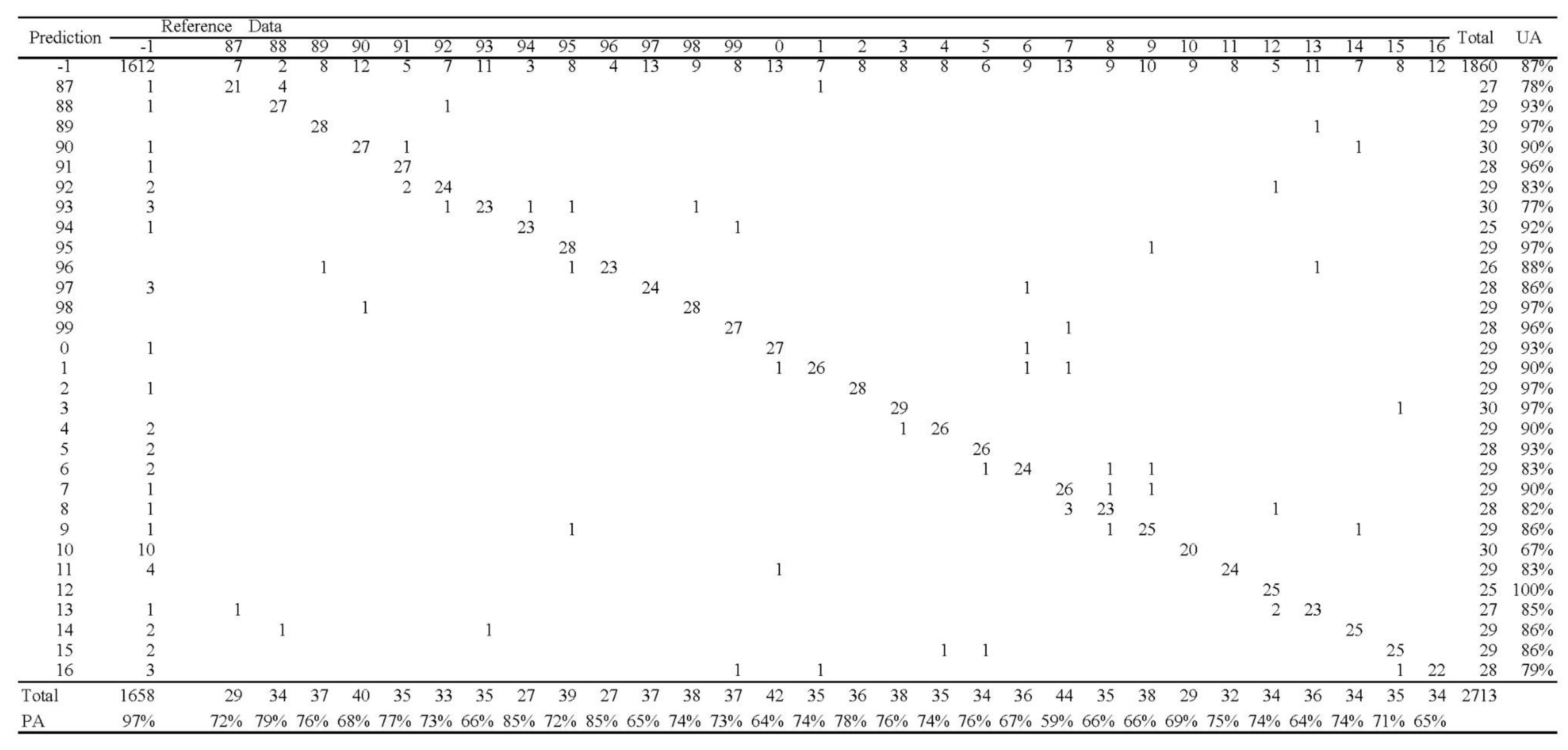
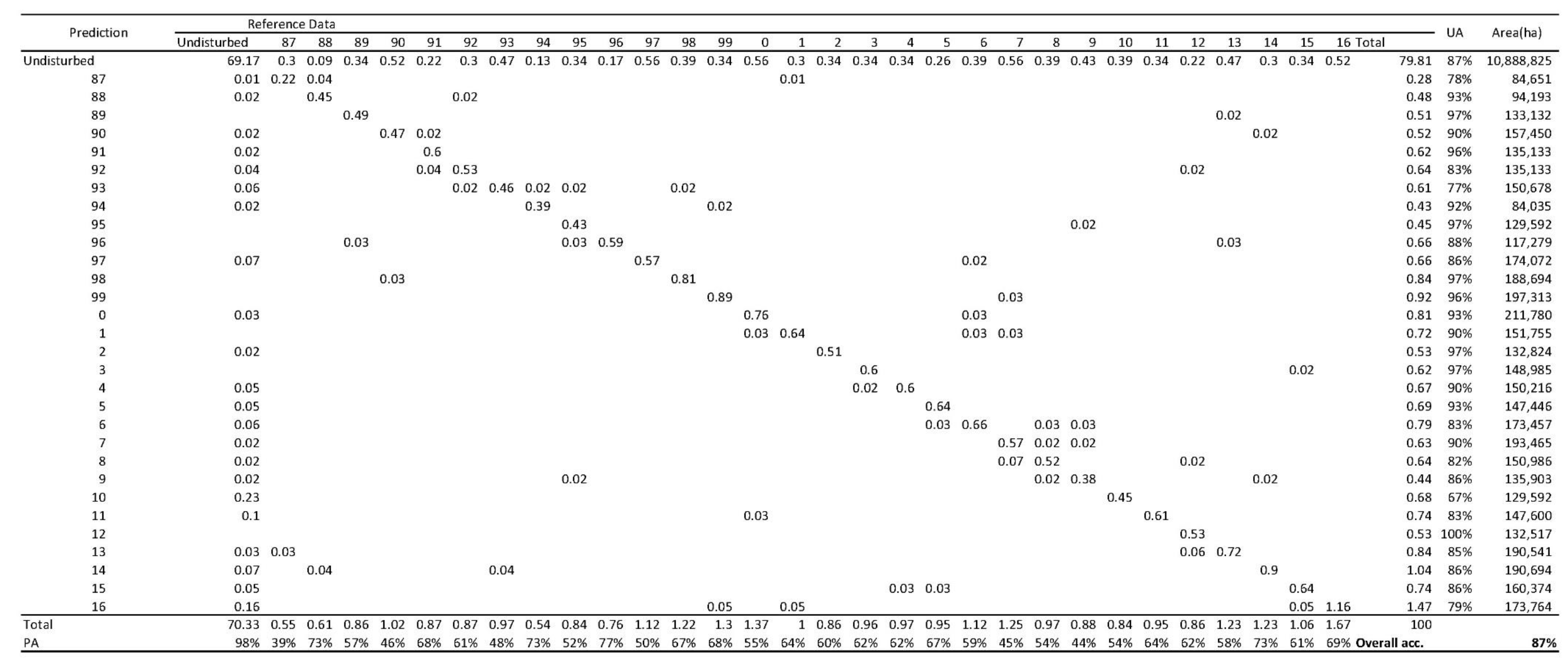
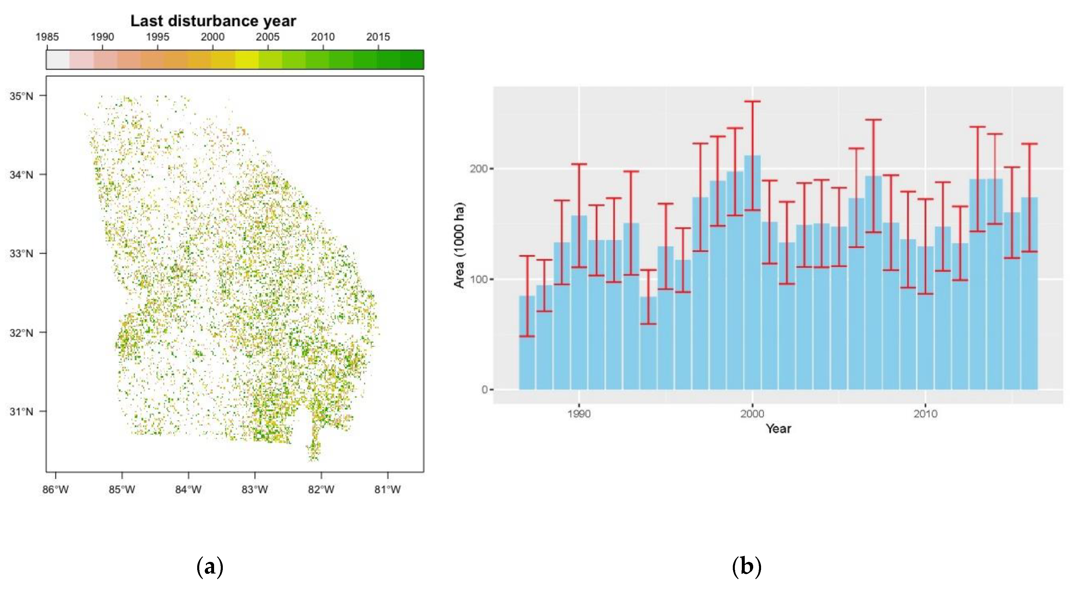
A 30-m spatial resolution raster database, in which each pixel was assigned a value that represents the last disturbance year of the forest (Figure 3a), was created as a result of applying the GEE to a time series of Landsat data. As is explained in Section 2.4, a count-based confusion matrix was developed to gauge the accuracy assessment (Figure A1). An area-adjusted confusion matrix was also developed to inform the accuracy assessment (Figure A2). Using the area-adjusted method, the overall accuracy was 87%. As was shown in Figure A1, when using the area-adjusted method, the commission rate was lower than the omission rate for most of the disturbed classes. Conversely, the commission rate was higher than the omission rate for the undisturbed classes. The high omission rate indicates that the disturbance detection algorithm tends to underestimate the area of disturbance.
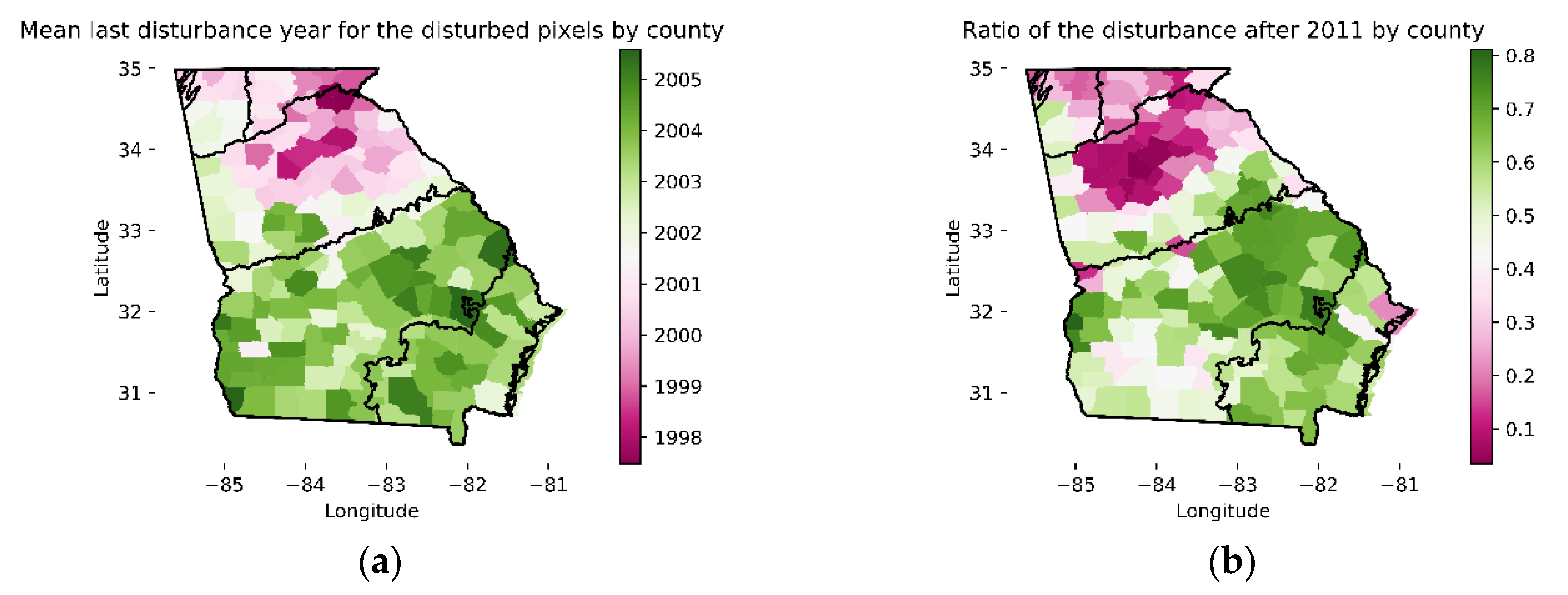
The estimated amount of disturbed area by disturbance year is plotted in Figure 3b. The estimate indicated that 4,503,253 ha of the forest land in Georgia, which occupies approximately 29.2% of the total forest land, was disturbed at least once between 1987 and 2016. The annual amount of disturbance area ranged between 84,651 ha (±36,354 ha) and 211,780 ha (±49,504 ha) for the entire state. It is worth mentioning that the annual last disturbance area tends to be lower in the early period of the time horizon of this research. Conversely, the annual last disturbance area tends to be larger for more recent years. This is because the recent disturbances overwrite the older disturbance record. To examine the regional variations in forest disturbances, we aggregated the pixel values of the temporal trajectory raster data to county-scale. The mean last disturbance year was then computed for each county, using pixels that have a disturbance record (Figure 4a). Subsequently, county-scale data was further aggregated at the ecoregion-scale (Table 3) to illustrate the mean last disturbance year for the 159 counties in the state. The mean last disturbance year was approximately 2003.69 for Southern Coastal Plain, while that of Blue Ridge ecoregion was 2000.11. This result indicates that the forest was disturbed more frequently in the areas where intensive management of plantations occupies more land.
To further examine the types of disturbances, the ratio of the recent disturbance subclass to the disturbed non-forest class (Figure 4b) was mapped. Figure 4b indicates that the majority of non-forest pixels with a disturbance record in the Southern Coastal Plain were disturbed after 2011. In these 19 counties located in the Southern Coastal Plain, more than 70% of the non-forest land was disturbed since 2011. On the other hand, about 67% of the non-forest land in Piedmont was disturbed during this time period. This result coincides with previous research, which revealed that the growth of the Atlanta metropolitan area over the last four decades has led to changes in land-use and the fragmentation of forests for urbanization purposes [52].

4. Discussion

In this research, we examined the recent forest disturbance history of the state of Georgia. In comparison to the change detection research that employed the VCT algorithm in North Carolina [53], our results have almost the same overall accuracy (88.6% vs. 87%), although the accuracy assessment methods between two research models are not identical. The most significant difference between the model in [53] and our model is the number of Landsat time series scenes used to conduct the analysis. As a result, our model less frequently misclassifies the disturbance year, plus or minus one year. This may be because we used all available imagery with less than 50% cloud cover. Due to the improved data availability, it was possible to detect forest disturbances approximately every 30 days, unlike the previous research that used a single set of imagery or mosaic imagery captured only during the growing season.
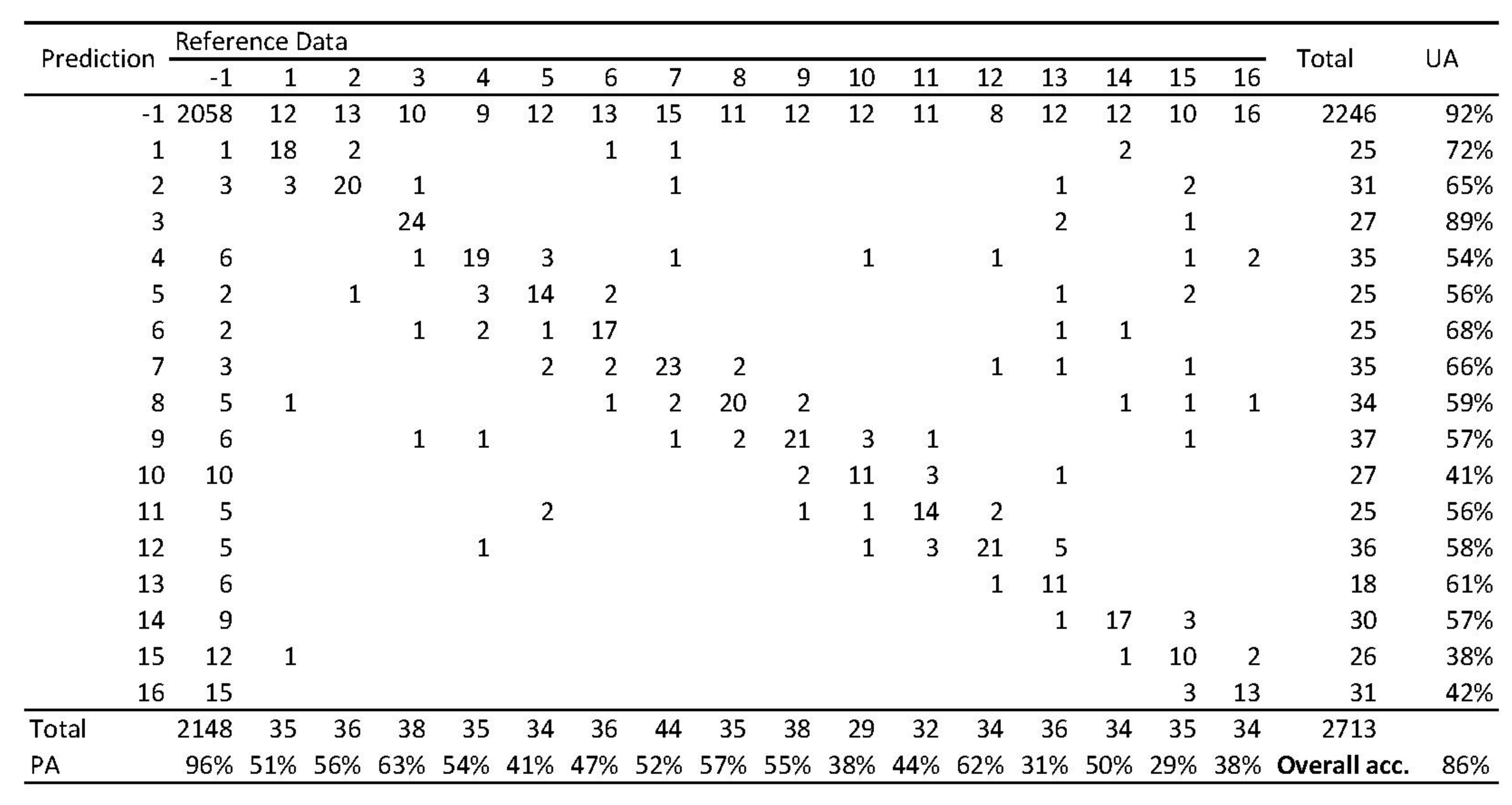
We attempted to compare our result with the two existing disturbance detection datasets: the North American Forest Dynamics data set [28] and the Global Forest Change dataset [19,54]. The North American Forest Dynamics dataset does not match the spatio-temporal range of our study, as it covered only two out of 14 WRS-2 scenes used in our research. Additionally, the North American Forest Dynamic dataset was limited to detecting change from 1986–2010. On the other hand, the Global Forest Change dataset includes the entire state of Georgia, although its temporal coverage initiates only after the year 2001. Thus, we selected the Global Forest Change dataset as the basis of the comparison. Version 1.4 of the Global Forest Change dataset was selected among the several available versions, as it covers the years extending between 2000 and 2016. If an accuracy assessment point was assigned a value smaller than that found in 2001, we reclassified it to the undisturbed class. Following this, the pixel values of the band that represents the year of gross forest cover loss event in the Global Forest Change dataset were extracted to the accuracy assessment points. Finally, a confusion matrix was constructed (Figure A3). The overall accuracy of Global Forest Change was 85.9%, which is lower than our result. Most of the user’s and producer’s accuracies for the disturbance class in Figure A3 were lower than our result, except for the undisturbed class.
The four conditions described in our new algorithm served different roles in detecting forest disturbances. Among these conditions, two of them, namely the backward and forward-moving average of IFZ, are based on the threshold method, while a third is based on the statistical boundary method. The backward moving average is a condition that quantifies the likelihood of a pixel being forest three years before the target date. The forward-moving average, on the other hand, quantifies the likelihood of a pixel being forest three years after the target date. These two moving averages describe the state of the landscape within a time frame. As is shown in the various research conducted concerning change detection models, it is possible to detect the occurrence of the land-use change by using only the backward and forward-moving averages [55,56,57]. However, if only these two conditions are employed, our algorithm suggests that disturbances are detected before they actually occur. This is because the forward-moving average exceeds the threshold when most of the observations come from the post-disturbance period. The final condition, which sets the statistical boundary for the five post-disturbance observations, helps to detect disturbances at the correct time. Therefore, combining the threshold method and the statistical boundary method alleviates the limitations of each method individually.
Although the results of the accuracy assessment suggest that this new method is better than our previous analysis, which attempted to detect the disturbance history of seven counties in Coastal Georgia [20], our new method still contained several areas of concern. For instance, on the commission error side of the analysis, we found that some forest thinnings could have been misclassified as a final harvest disturbance. One possible reason for the confusion is that the change in IFZ, when mediated through a high intensity thinning and through a final disturbance, could be similar due to the amount of forest canopy removed, the amount of forest floor exposed, and the size of Landsat pixels. Often, a forest thinning in plantation forests in Georgia removes up to 50% of the basal area, and the residual live tree canopy may require three years or more to close the gaps that are created. Conversely, on the omission error side, omission error rates for the disturbance classes were between 23% to 67% in the area-adjusted confusion matrix. These errors are often physically located at the edges of the disturbed stands. The omission error rate could be reduced by changing the threshold values set for our disturbance detection algorithm. However, a more relaxed set of threshold values for the disturbance detection process might result in a higher commission error rate by confusing thinnings with final harvest disturbances. Thus, a delicate balance must be achieved if the parameters are to be adjusted in an effort to reduce omission or commission errors. One plausible way of acquiring better overall accuracy may be to develop a system that would optimize the threshold values in the conditions we set in our algorithm.
Future research related to the methods described here might focus on detecting more recent disturbances. To achieve this goal, it is necessary to remove the third and fourth conditions in our model, which observe the IFZ values after the disturbance. A second focus may be to combine the regeneration history data with disturbance year, as the timing of regeneration processes (site preparation, planting, etc.) can range from nearly instantaneous after harvest, to 2–3 years after harvest. In our regional-scale disturbance analysis, we did not directly examine the timing of forest regeneration. By applying a method for detecting the forest regeneration, it is expected that one may more closely comprehend dynamic changes in forests across broad areas of a landscape.
Finally, the disturbance year map created in this research can be used to conduct an analysis related to the forest inventory in Georgia. Once the disturbance year is combined with a broad-scale forest inventory, the data can be used to estimate the above-ground biomass and perhaps other forest product-related metrics of interest to both society and industry. Previous research has demonstrated the use of these types of methods in estimating biomass in various regions by incorporating environmental data to improve the accuracy of the estimation [58,59,60,61]. Although these research efforts have succeeded in creating databases that estimate above-ground biomass, there is a known issue in which spectral reflectance values of Landsat imagery are insensitive to changes in biomass among dense and multilayered canopy forests, regardless of their age. Consequently, the biomass estimation results in low accuracy for high biomass stands [62,63]. By incorporating the disturbance year data created in this research, it is expected that the old forest and young forest can be discriminated more easily among dense and multilayered canopy forests.

5. Conclusions

In this research, we established a high-resolution, spatially explicit inventory of Georgia’s forest disturbance history that will serve as a baseline for stand-level forest management and conservation. The raster database we created presents the last disturbance year of forests. Then, Google Earth Engine was used to process all available images from the time series of Landsat TM/ETM+ imagery. Finally, we combined the VCT algorithm, a threshold method, and the statistical boundary method to create our algorithm, which detects forest disturbances. The overall accuracy of the disturbance year data was 87%. The data suggests that 29.2% of the land area in Georgia was disturbed between 1987 and 2016. The estimated annual last disturbance area ranged between 84,651 ± 36,354 ha and 211,780 ± 49,504 ha. As the process records only the final disturbance for each pixel, the annual area of disturbance tends to increase towards the more recent years. The use of all available time-series Landsat imagery contributed to the achievement of less frequent misclassification of the disturbance year, plus or minus one year. Combining the threshold method and the statistical boundary method made it possible to detect disturbances with a relatively accurate temporal specification. Furthermore, by using the NLCD 2016 dataset and the disturbance map we created, we were able to further examine regional variations in the disturbance history. The subsequent analysis confirmed common insight on land-use patterns: namely, that disturbed forests near urban areas were more likely to be converted to other land-uses than disturbed forests in rural areas. Meanwhile, in the Southern Coastal Plain, where intensive plantation forest management is widely practiced, forests experienced the greatest intensity of disturbance and regenerated at a higher rate relative to other regions.

Author Contributions

Conceptualization, P.B. and C.J.C.; methodology, S.O. and C.J.C.; programming, S.O. and R.C.L.III; validation, S.O.; formal analysis, S.O.; investigation, S.O.; resources, S.O.; data curation, S.O.; writing—original draft preparation, S.O.; writing—review and editing, P.B., C.J.C. and R.C.L.III; visualization, S.O.; supervision, P.B. and C.J.C.; project administration, P.B. and R.C.L.III; funding acquisition, S.O. All authors have read and agreed to the published version of the manuscript.

Funding

We are indebted to the Japan Student Service Organization Student Exchange Support Program (Graduate Scholarship for Degree Seeking Students) for funding this research. This work was also supported by the United States Department of Agriculture, National Institute of Food and Agriculture, McIntire-Stennis project (1012166), administered by the Warnell School of Forestry and Natural Resources at the University of Georgia.

Acknowledgments

We would also like to mention our appreciation for the support and assistance of the Google Earth Engine Development team.

Conflicts of Interest

The authors declare no conflict of interest.

Appendix A

Figure A1. Count-based confusion matrix. Reference data and prediction class values represent the last disturbance year (e.g., 89 = year 1989). The −1 class represents the undisturbed class. UA = user’s accuracy. PA = producer’s accuracy.
Forests 11 00335 g0a1
Figure A2. Area-adjusted confusion matrix. Reference data and prediction class values represent the last disturbance year (e.g., 89 = year 1989). The −1 class represents the undisturbed class. UA = user’s accuracy. PA = producer’s accuracy.
Forests 11 00335 g0a2
Figure A3. Count-based confusion matrix for Global Forest Change Version 1.4 data set. Reference data and prediction class values represent the last disturbance year (e.g., 01 = year 2001). The −1 class represents the undisturbed class. UA = user’s accuracy. PA = producer’s accuracy.
Forests 11 00335 g0a3

References

  1. Pflugmacher, D.; Cohen, W.B.; Kennedy, R.E. Using Landsat-derived disturbance history (1972–2010) to predict current forest structure. Remote Sens. Environ. 2012, 122, 146–165. [Google Scholar] [CrossRef]
  2. Edwards, D.P.; Tobias, J.A.; Sheil, D.; Meijaard, E.; Laurance, W.F. Maintaining ecosystem function and services in logged tropical forests. Trends Ecol. Evol. 2014, 29, 511–520. [Google Scholar] [CrossRef] [Green Version]
  3. Zhu, Z.; Zhang, J.; Yang, Z.; Aljaddani, A.H.; Cohen, W.B.; Qiu, S.; Zhou, C. Continuous monitoring of land disturbance based on Landsat time series. Remote Sens. Environ. 2019, 238, 111116. [Google Scholar] [CrossRef]
  4. Goldenberg, S.B.; Landsea, C.W.; Mestas-Nuñez, A.M.; Gray, W.M. The recent increase in Atlantic hurricane activity: Causes and implications. Science 2001, 293, 474–479. [Google Scholar] [CrossRef] [Green Version]
  5. Zampieri, N.E.; Pau, S.; Okamoto, D.K. The impact of Hurricane Michael on longleaf pine habitats in Florida. bioRxiv 2019. [Google Scholar] [CrossRef] [Green Version]
  6. Williams, C.A.; Gu, H.; MacLean, R.; Masek, J.G.; Collatz, G.J. Disturbance and the carbon balance of US forests: A quantitative review of impacts from harvests, fires, insects, and droughts. Glob. Planet. Chang. 2016, 143, 66–80. [Google Scholar] [CrossRef]
  7. Westerling, A.L.; Hidalgo, H.G.; Cayan, D.R.; Swetnam, T.W. Warming and earlier spring increase western U.S. forest wildfire activity. Science 2006, 313, 940–943. [Google Scholar] [CrossRef] [PubMed] [Green Version]
  8. Seidl, R.; Schelhaas, M.-J.; Rammer, W.; Verkerk, P.J. Increasing forest disturbances in Europe and their impact on carbon storage. Nat. Clim. Chang. 2014, 4, 806–810. [Google Scholar] [CrossRef] [PubMed] [Green Version]
  9. Grogan, K.; Pflugmacher, D.; Hostert, P.; Kennedy, R.; Fensholt, R. Cross-border forest disturbance and the role of natural rubber in mainland southeast Asia using annual Landsat time series. Remote Sens. Environ. 2015, 169, 438–453. [Google Scholar] [CrossRef]
  10. Cohen, W.B.; Yang, Z.; Stehman, S.V.; Schroeder, T.A.; Bell, D.M.; Masek, J.G.; Huang, C.; Meigs, G.W. Forest disturbance across the conterminous United States from 1985–2012: The emerging dominance of forest decline. For. Ecol. Manag. 2016, 360, 242–252. [Google Scholar] [CrossRef]
  11. Oswalt, S.N.; Smith, W.B.; Miles, P.D.; Pugh, S.A. Forest Resources of the United States, 2017; General Technical Report WO-97; United States Department of Agriculture, Forest Service: Washington, DC, USA, 2018.
  12. Nilsson, U.; Allen, H.L. Short- and long-term effects of site preparation, fertilization and vegetation control on growth and stand development of planted loblolly pine. For. Ecol. Manag. 2003, 175, 367–377. [Google Scholar] [CrossRef]
  13. D’Amato, A.W.; Jokela, E.J.; O’Hara, K.L.; Long, J.N. Silviculture in the United States: An amazing period of change over the past 30 years. J. For. 2017, 116, 55–67. [Google Scholar] [CrossRef] [Green Version]
  14. Fox, T.R.; Jokela, E.J.; Allen, H.L. The development of pine plantation silviculture in the Southern United States. J. For. 2007, 105, 337–347. [Google Scholar]
  15. Hairston-Strang, A.B.; Adams, P.W.; Ice, G.G. The Oregon Forest Practices Act and Forest research. In Hydrological and Biological Responses to Forest Practices; Stednick, J.D., Ed.; Springer: New York, NY, USA, 2008; Volume 199, pp. 95–113. ISBN 978-0-387-94385-5. [Google Scholar]
  16. Prud’homme, B.A.; Greis, J.G. Best Management Practices in the South. In Southern Forest Resource Assessment; General Technical Report SRS-53; Department of Agriculture, Forest Service, Southern Research Station: Asheville, NC, USA, 2002; pp. 519–536. [Google Scholar]
  17. Cieszewski, C.J.; Zasada, M.; Borders, B.E.; Lowe, R.C.; Zawadzki, J.; Clutter, M.L.; Daniels, R.F. Spatially explicit sustainability analysis of long-term fiber supply in Georgia, USA. For. Ecol. Manag. 2004, 187, 349–359. [Google Scholar] [CrossRef]
  18. Liu, S.; Cieszewski, C.J. Impacts of management intensity and harvesting practices on long-term forest resource sustainability in Georgia. Math. Comput. For. Nat.-Resour. Sci. 2009, 1, 52–66. [Google Scholar]
  19. Hansen, M.C.; Potapov, P.V.; Moore, R.; Hancher, M.; Turubanova, S.A.; Tyukavina, A.; Thau, D.; Stehman, S.V.; Goetz, S.J.; Loveland, T.R.; et al. High-resolution global maps of 21st-Century forest cover change. Science 2013, 342, 850–853. [Google Scholar] [CrossRef] [PubMed] [Green Version]
  20. Obata, S.; Cieszewski, C.J.; Bettinger, P.; Lowe, R.C., III; Bernardes, S. Preliminary analysis of forest stand disturbances in Coastal Georgia (USA) using Landsat time series stacked imagery. Formath 2019, 18, 1–11. [Google Scholar] [CrossRef]
  21. Zhu, Z.; Woodcock, C.E.; Olofsson, P. Continuous monitoring of forest disturbance using all available Landsat imagery. Remote Sens. Environ. 2012, 122, 75–91. [Google Scholar] [CrossRef]
  22. Huang, C.; Goward, S.N.; Masek, J.G.; Thomas, N.; Zhu, Z.; Vogelmann, J.E. An automated approach for reconstructing recent forest disturbance history using dense Landsat time series stacks. Remote Sens. Environ. 2010, 114, 183–198. [Google Scholar] [CrossRef]
  23. Kennedy, R.E.; Andréfouët, S.; Cohen, W.B.; Gómez, C.; Griffiths, P.; Hais, M.; Healey, S.P.; Helmer, E.H.; Hostert, P.; Lyons, M.B.; et al. Bringing an ecological view of change to Landsat-based remote sensing. Front. Ecol. Environ. 2014, 12, 339–346. [Google Scholar] [CrossRef]
  24. Woodcock, C.E.; Allen, R.; Anderson, M.; Belward, A.; Bindschadler, R.; Cohen, W.; Gao, F.; Goward, S.N.; Helder, D.; Helmer, E.; et al. Free access to Landsat imagery. Science 2008, 320, 1011. [Google Scholar] [CrossRef] [PubMed]
  25. Wulder, M.A.; Masek, J.G.; Cohen, W.B.; Loveland, T.R.; Woodcock, C.E. Opening the archive: How free data has enabled the science and monitoring promise of Landsat. Remote Sens. Environ. 2012, 122, 2–10. [Google Scholar] [CrossRef]
  26. Loveland, T.R.; Dwyer, J.L. Landsat: Building a strong future. Remote Sens. Environ. 2012, 122, 22–29. [Google Scholar] [CrossRef]
  27. Wulder, M.A.; White, J.C.; Loveland, T.R.; Woodcock, C.E.; Belward, A.S.; Cohen, W.B.; Fosnight, E.A.; Shaw, J.; Masek, J.G.; Roy, D.P. The global Landsat archive: Status, consolidation, and direction. Remote Sens. Environ. 2016, 185, 271–283. [Google Scholar] [CrossRef] [Green Version]
  28. Masek, J.G.; Goward, S.N.; Kennedy, R.E.; Cohen, W.B.; Moisen, G.G.; Schleeweis, K.; Huang, C. United States forest disturbance trends observed using Landsat time series. Ecosystems 2013, 16, 1087–1104. [Google Scholar] [CrossRef] [Green Version]
  29. Kennedy, R.E.; Yang, Z.; Cohen, W.B. Detecting trends in forest disturbance and recovery using yearly Landsat time series: 1. LandTrendr — Temporal segmentation algorithms. Remote Sens. Environ. 2010, 114, 2897–2910. [Google Scholar] [CrossRef]
  30. Li, M.; Huang, C.; Zhu, Z.; Wen, W.; Xu, D.; Liu, A. Use of remote sensing coupled with a vegetation change tracker model to assess rates of forest change and fragmentation in Mississippi, USA. Int. J. Remote Sens. 2009, 30, 6559–6574. [Google Scholar] [CrossRef]
  31. Zhu, Z. Change detection using Landsat time series: A review of frequencies, preprocessing, algorithms, and applications. ISPRS J. Photogramm. Remote Sens. 2017, 130, 370–384. [Google Scholar] [CrossRef]
  32. Brooks, E.B.; Wynne, R.H.; Thomas, V.A.; Blinn, C.E.; Coulston, J.W. On-the-fly massively multitemporal change detection using statistical quality control charts and Landsat data. IEEE Trans. Geosci. Remote Sens. 2014, 52, 3316–3332. [Google Scholar] [CrossRef]
  33. DeVries, B.; Decuyper, M.; Verbesselt, J.; Zeileis, A.; Herold, M.; Joseph, S. Tracking disturbance-regrowth dynamics in tropical forests using structural change detection and Landsat time series. Remote Sens. Environ. 2015, 169, 320–334. [Google Scholar] [CrossRef]
  34. Zhu, Z.; Fu, Y.; Woodcock, C.E.; Olofsson, P.; Vogelmann, J.E.; Holden, C.; Wang, M.; Dai, S.; Yu, Y. Including land cover change in analysis of greenness trends using all available Landsat 5, 7, and 8 images: A case study from Guangzhou, China (2000–2014). Remote Sens. Environ. 2016, 185, 243–257. [Google Scholar] [CrossRef] [Green Version]
  35. Gorelick, N.; Hancher, M.; Dixon, M.; Ilyushchenko, S.; Thau, D.; Moore, R. Google Earth Engine: Planetary-scale geospatial analysis for everyone. Remote Sens. Environ. 2017, 202, 18–27. [Google Scholar] [CrossRef]
  36. Shelestov, A.; Lavreniuk, M.; Kussul, N.; Novikov, A.; Skakun, S. Exploring Google Earth Engine platform for big data processing: Classification of multi-temporal satellite imagery for crop mapping. Front. Earth Sci. 2017, 5. [Google Scholar] [CrossRef] [Green Version]
  37. Huang, H.; Chen, Y.; Clinton, N.; Wang, J.; Wang, X.; Liu, C.; Gong, P.; Yang, J.; Bai, Y.; Zheng, Y.; et al. Mapping major land cover dynamics in Beijing using all Landsat images in Google Earth Engine. Remote Sens. Environ. 2017, 202, 166–176. [Google Scholar] [CrossRef]
  38. Johansen, K.; Phinn, S.; Taylor, M. Mapping woody vegetation clearing in Queensland, Australia from Landsat imagery using the Google Earth Engine. Remote Sens. Appl. Soc. Environ. 2015, 1, 36–49. [Google Scholar] [CrossRef]
  39. Lambert, S.; Brandeis, T. Forests of Georgia, 2016. Resource Update FS–176; United States Department of Agriculture, Forest Service, Southern Research Station: Asheville, NC, USA, 2018.
  40. Omernik, J.M.; Griffith, G.E. Ecoregions of the conterminous United States: Evolution of a hierarchical spatial framework. Environ. Manag. 2014, 54, 1249–1266. [Google Scholar] [CrossRef]
  41. US Census Bureau. Metropolitan and Micropolitan Statistical Areas Totals: 2010–2018. Available online: https://www.census.gov/data/tables/time-series/demo/popest/2010s-total-metro-and-micro-statistical-areas.html (accessed on 19 August 2019).
  42. Edwards, L.; Ambrose, J.; Kirkman, L.K. The Natural Communities of Georgia; University of Georgia Press: Athens, GA, USA, 2013; ISBN 978-0-8203-3021-1. [Google Scholar]
  43. Roy, D.P.; Wulder, M.A.; Loveland, T.R.; Woodcock, C.E.; Allen, R.G.; Anderson, M.C.; Helder, D.; Irons, J.R.; Johnson, D.M.; Kennedy, R.; et al. Landsat-8: Science and product vision for terrestrial global change research. Remote Sens. Environ. 2014, 145, 154–172. [Google Scholar] [CrossRef] [Green Version]
  44. Foga, S.; Scaramuzza, P.L.; Guo, S.; Zhu, Z.; Dilley, R.D.; Beckmann, T.; Schmidt, G.L.; Dwyer, J.L.; Hughes, M.J.; Laue, B. Cloud detection algorithm comparison and validation for operational Landsat data products. Remote Sens. Environ. 2017, 194, 379–390. [Google Scholar] [CrossRef] [Green Version]
  45. Zhu, Z.; Wang, S.; Woodcock, C.E. Improvement and expansion of the Fmask algorithm: Cloud, cloud shadow, and snow detection for Landsats 4–7, 8, and Sentinel 2 images. Remote Sens. Environ. 2015, 159, 269–277. [Google Scholar] [CrossRef]
  46. Zhu, Z.; Woodcock, C.E. Object-based cloud and cloud shadow detection in Landsat imagery. Remote Sens. Environ. 2012, 118, 83–94. [Google Scholar] [CrossRef]
  47. Zhu, Z.; Woodcock, C.E. Continuous change detection and classification of land cover using all available Landsat data. Remote Sens. Environ. 2014, 144, 152–171. [Google Scholar] [CrossRef] [Green Version]
  48. Card, D.H. Using known map category marginal frequencies to improve estimates of thematic map accuracy. Photogramm. Eng. Remote Sens. 1982, 48, 431–439. [Google Scholar]
  49. Olofsson, P.; Foody, G.M.; Stehman, S.V.; Woodcock, C.E. Making better use of accuracy data in land change studies: Estimating accuracy and area and quantifying uncertainty using stratified estimation. Remote Sens. Environ. 2013, 129, 122–131. [Google Scholar] [CrossRef]
  50. Yang, L.; Jin, S.; Danielson, P.; Homer, C.; Gass, L.; Bender, S.M.; Case, A.; Costello, C.; Dewitz, J.; Fry, J.; et al. A new generation of the United States National Land Cover Database: Requirements, research priorities, design, and implementation strategies. ISPRS J. Photogramm. Remote Sens. 2018, 146, 108–123. [Google Scholar] [CrossRef]
  51. Multi-Resolution Land Characteristics Consortium. NLCD 2016 Land Cover. Available online: https://www.mrlc.gov/data/nlcd-2016-land-cover-conus (accessed on 30 September 2019).
  52. Miller, M.D. The impacts of Atlanta’s urban sprawl on forest cover and fragmentation. Appl. Geogr. 2012, 34, 171–179. [Google Scholar] [CrossRef]
  53. Huang, C.; Ling, P.-Y.; Zhu, Z. North Carolina’s forest disturbance and timber production assessed using time series Landsat observations. Int. J. Digit. Earth 2015, 8, 947–969. [Google Scholar] [CrossRef] [Green Version]
  54. Hansen, M.C.; Stehman, S.V.; Potapov, P.V. Quantification of global gross forest cover loss. Proc. Natl. Acad. Sci. USA 2010, 107, 8650–8655. [Google Scholar] [CrossRef] [Green Version]
  55. Pickell, P.D.; Hermosilla, T.; Coops, N.C.; Masek, J.G.; Franks, S.; Huang, C. Monitoring anthropogenic disturbance trends in an industrialized boreal forest with Landsat time series. Remote Sens. Lett. 2014, 5, 783–792. [Google Scholar] [CrossRef]
  56. Li, J.; Zipper, C.E.; Donovan, P.F.; Wynne, R.H.; Oliphant, A.J. Reconstructing disturbance history for an intensively mined region by time-series analysis of Landsat imagery. Environ. Monit. Assess. 2015, 187, 557. [Google Scholar] [CrossRef]
  57. Kayastha, N.; Thomas, V.; Galbraith, J.; Banskota, A. Monitoring wetland change using inter-annual Landsat time-series data. Wetlands 2012, 32, 1149–1162. [Google Scholar] [CrossRef]
  58. Tanaka, S.; Takahashi, T.; Nishizono, T.; Kitahara, F.; Saito, H.; Iehara, T.; Kodani, E.; Awaya, Y. Stand volume estimation using the k-NN technique combined with forest inventory data, satellite image data and additional feature variables. Remote Sens. 2014, 7, 378–394. [Google Scholar] [CrossRef] [Green Version]
  59. McRoberts, R.E. Estimating forest attribute parameters for small areas using nearest neighbors techniques. For. Ecol. Manag. 2012, 272, 3–12. [Google Scholar] [CrossRef]
  60. Tomppo, E.; Olsson, H.; Ståhl, G.; Nilsson, M.; Hagner, O.; Katila, M. Combining national forest inventory field plots and remote sensing data for forest databases. Remote Sens. Environ. 2008, 112, 1982–1999. [Google Scholar] [CrossRef]
  61. Maselli, F.; Chirici, G.; Bottai, L.; Corona, P.; Marchetti, M. Estimation of Mediterranean forest attributes by the application of k-NN procedures to multitemporal Landsat ETM+ images. Int. J. Remote Sens. 2005, 26, 3781–3796. [Google Scholar] [CrossRef] [Green Version]
  62. Lu, D.; Chen, Q.; Wang, G.; Liu, L.; Li, G.; Moran, E. A survey of remote sensing-based aboveground biomass estimation methods in forest ecosystems. Int. J. Digit. Earth 2016, 9, 63–105. [Google Scholar] [CrossRef]
  63. Zhao, P.; Lu, D.; Wang, G.; Wu, C.; Huang, Y.; Yu, S. Examining spectral reflectance saturation in Landsat imagery and corresponding solutions to improve forest aboveground biomass estimation. Remote Sens. 2016, 8, 469. [Google Scholar] [CrossRef] [Green Version]
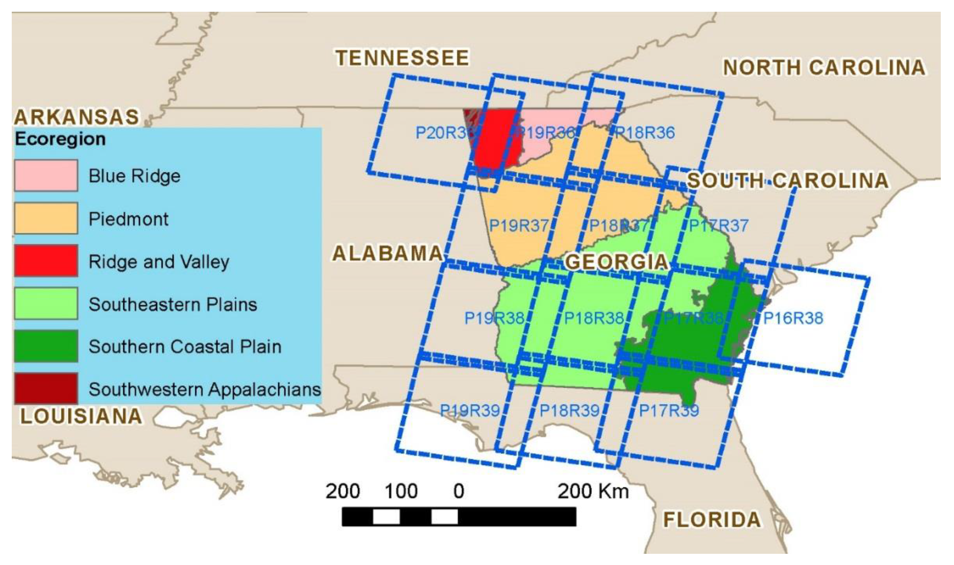
Figure 1. Study area. The combination of letter and number in the figure represents the path and row number of World Reference System-2 (WRS-2).
Forests 11 00335 g001
Figure 2. Change in time series Integrated Forest z-score (IFZ) values (Lat: 32.097°, Lon: −84.844°).
Forests 11 00335 g002
Figure 3. (a) The last disturbance year map. (b) Estimated area distribution of the last disturbance year.
Forests 11 00335 g003
Figure 4. Disturbance pattern classification maps by county. (a) Mean last disturbance year for the disturbed pixels (b) Ratio of the disturbance after 2011 to all of the disturbances detected between 1987–2016.
Forests 11 00335 g004
Table 1. Dense Landsat time-series data summary by scenes. Four-digit numbers at the header represent the WRS-2 row/path combination of the scene. The first two digits represent the path number and the following two digits represent the row number (e.g., “1638” refers to path 16 and row 38). The “number (#) of images” row represents the total number of available images for each scene captured between April 1984 and December 2016. The “Days/Image” row represents the average length of time from the acquisition of an image to the acquisition of the next image in Google Earth Engine (GEE).
Values/Scene1638173717381739183618371838183919361937193819392036Mean
Mean Cloud %15.012.614.017.214.313.214.214.915.413.614.714.414.714.5
# of images446419440453440429442436412429449446373431.9
Days/Image27.028.827.426.627.428.127.327.629.328.126.827.032.328.0
Table 2. Disturbance history classification class.
Class NameNLCD ClassDisturbanceArea (ha)Description
1Disturbed forestForestBetween 1987–20162,347,978Disturbed at least once, currently forested
2Persistent forestForestNo disturbance7,330,405 Persistent forest
3Recent disturbanceNon-Forest2011–2016370,208Disturbed after 2011, currently non-forest
4Persistent non-forestNon-ForestNo disturbance4,944,445 Persistent non-forest
5DeforestationNon-Forest1987–2010398,663Disturbed before 2011, currently non-forest
Table 3. Land-use pattern classification in Georgia.
EcoregionDistForPerForRecDistPerNonDeforAvgYear
Blue Ridge3.5176.470.3618.361.312000.11
Piedmont11.8350.231.5233.183.232000.93
Ridge and Valley9.0752.701.0235.301.922001.12
Southeastern Plains15.4842.732.8037.211.792003.68
Southern Coastal Plain23.2745.184.5523.963.062003.69
DistFor: Disturbed forest (%); PerFor: Persistent forest (%); RecDist: Recent disturbance (%); PerNon: Persistent non-forest (%); DeFor: Deforestation (%); AvgYear: Mean last disturbance year.