Abstract
Accurate estimation of tree biomass is required for accounting for and monitoring forest carbon stocking. Allometric biomass equations constructed by classical statistical methods are widely used to predict tree biomass in forest ecosystems. In this study, a Bayesian approach was proposed and applied to develop two additive biomass model systems: one with tree diameter at breast height as the only predictor and the other with both tree diameter and total height as the predictors for planted Korean larch (Larix olgensis Henry) in the Northeast, P.R. China. The seemingly unrelated regression (SUR) was used to fit the simultaneous equations of four tree components (i.e., stem, branch, foliage, and root). The model parameters were estimated by feasible generalized least squares (FGLS) and Bayesian methods using either non-informative priors or informative priors. The results showed that adding tree height to the model systems improved the model fitting and performance for the stem, branch, and foliage biomass models, but much less for the root biomass models. The Bayesian methods on the SUR models produced narrower 95% prediction intervals than did the classical FGLS method, indicating higher computing efficiency and more stable model predictions, especially for small sample sizes. Furthermore, the Bayesian methods with informative priors performed better (smaller values of deviance information criterion (DIC)) than those with the non-informative priors. Therefore, our results demonstrated the advantages of applying the Bayesian methods on the SUR biomass models, not only obtaining better model fitting and predictions, but also offering the assessment and evaluation of the uncertainties for constructing and updating tree biomass models.
1. Introduction
In the practice of sustainable forest management, tree biomass is primarily used to calculate the carbon storage and sequestration of forests and further to comprehend climate change and forest health, productivity, and nutrient cycling [1,2]. It is well known that the most appropriate method for estimating tree biomass is to use biomass models developed using the direct measurements of tree biomass (response variable) and predictor variables [3,4]. Over the past decades, hundreds of biomass equations have been developed for different tree species around the world [5,6,7]. Tree diameter at breast height (DBH) is the commonly used predictor variable, which is considered the readily attainable and most reliable sole predictor [8]. Tree height (H) is also used for developing biomass models to improve the model performance and explain the potential limitations of intra-species divergence [9,10]. The biomass models with both DBH and H are recognized more stable and reliable for predicting tree biomass [11,12]. Furthermore, various modeling approaches have been explored and applied for developing tree biomass models [13,14].
To date, the biomass of different tree components (i.e., stem, branch, foliage, and root) are usually estimated jointly in order to account for the inherent correlations among those tree components because they are measured within the same sample trees [11]. The additive model systems of either linear or nonlinear functions are used to deal with the correlations between the biomass components from the same tree, which are commonly known as seemingly unrelated regression (SUR) models [15]. Over the past decades, there are different parameter estimation methods proposed for the additive model systems from the perspective of traditional statistics, such as two-step feasible generalized least squares (FGLS), iterative FGLS (IFGLS), maximum likelihood (ML), etc. [16,17]. FGLS has been widely used for parameter estimation of the SUR models [18] and has been considered more favorable in recent years because of its simplicity and flexibility in practical applications [19]. However, it is recognized that those classical methods are not able to access and evaluate the uncertainty of parameter estimates and the reliability of model predictions.
Zellner [20] proposed the usage of Bayesian analyses in modeling practices to take advantage of Bayesian’s capability of estimating model parameters using probability statements and, consequently, fulfilling the purposes of uncertainty assessment [21]. In the past, however, the applications of the Bayesian approaches were limited due to the lack of numerical optimization theory and computing power. In addition, Bayesian methods can be readily applied to linear models, but many allometric relationships are nonlinear in nature. Following the widespread applications of the Markov Chain Monte Carlo (MCMC) method and rapid development of computing technology, Griffiths [22] finally implemented Bayesian methods for SUR models in the field of econometrics.
For many years, Bayesian theorem was not accepted and well recognized among researchers, even though it was proposed by Thomas Bayes in the mid-18th century [23]. Scientists began to accept and deepen their understanding of Bayesian modeling philosophy because it has unique benefits in solving some practical problems, which are highly supported by the remarkable escalation in computing power. The fundamental enhancement of applying Bayesian methods lies within their ability to create the full posterior distributions of model parameters; hence, several statistics (e.g., mean, median, quantiles, etc.) can be easily computed from the samples generated during the model fitting processes [24]. In addition, Bayesian methods consider the model parameters as random variables and assume that each parameter has a prior distribution, which then is naturally integrated with the sample information to obtain the posterior probability distribution for the parameter [25]. To date, Bayesian analysis is considered an essential and important element in modeling practices across many scientific fields, such as biology [26], engineering [27], finance [25], genetics [28], etc. In general, Bayesian analysis can be divided into two major categories, namely objective and subjective Bayesian methods, due to the types of prior distributions. The objective Bayesian method often uses a non-informative prior (e.g., Jeffreys prior), while the subjective Bayesian method utilizes humans’ perspective or other available information as an informative prior for estimating the model parameters [29]. However, questions still arise among researchers regarding the appropriate determination and selection of the prior distribution in Bayesian methods. In fact, this is one of the most debated issues by researchers, because it influences the computation and results of the posterior distribution [30]. In recent years, the MCMC method has initiated broad prospects for the promotion and application of Bayesian methods so that it has become a reliable tool for handling complex problems in statistics and modeling practices [31].
Bayesian methods have been widely applied in forestry research in recent years, including the studies of tree diameter and height growth, mortality, tree biomass, etc. [1,13,21,24]. Zapata-Cuartas [13] established the aboveground biomass model for the Colombian tropical forest using Bayesian approaches incorporating 132 biomass equations from 72 published articles as the prior information. Zhang et al. [32] utilized Bayesian approaches to estimate stem, branch, foliage, root, and total tree biomass models with both non-informative and informative priors. They proved that the Bayesian methods with informative priors produced better performances than those with non-informative priors and classical methods. In this sense, Bayesian statistics have the advantage of model performance in the case of fitting individual models. However, the biomass of different tree components is usually estimated jointly, while other studies found in published research were only based on a single biomass model, ignoring the inherent correlations among the biomass of tree components. Although the additive model systems with linear or nonlinear functions have been widely used and become a standard for developing individual tree biomass models [2,8], to the best of our knowledge, there has been no publication in the literature on the applications of Bayesian methods with SUR to jointly estimate the additive biomass model systems of tree components.
Korean larch is one of the most important fast-growing conifer species for timber production in the Northeast, P.R. China. The larch plantations encompass a wide range of geographical coverage, from the northeastern to the northern subalpine areas of China [33]. It is desirable and needed to maximize and maintain the ecological and economic benefits of the Korean larch plantations. Therefore, reliable biomass models with the capability of uncertainty assessment are necessary for estimating, accounting, and monitoring tree biomass and forest carbon stocking. In this study, we used data consisting of 174 destructively sampled Korean larch (Larix olgensis Henry) to develop the additive biomass model systems of tree components (i.e., stem, branch, foliage, and root) for planted Korean larch. Two additive model systems were constructed to facilitate the application of different data types; the first one used tree DBH as the only predictor, and the second one used both tree DBH and H as the predictors. For each model system, we compared two parameter estimation methods: classical FGLS (as the benchmark) and Bayesian methods. A comprehensive sample of allometric biomass equations for Larix spp. in different locations gathered from published literatures provided sufficient prior information of model parameters.
The objective of this study was to explore the advantages of Bayesian approaches on the SUR models of individual tree biomass. We expected that the SUR model systems using Bayesian methods would produce superior model fitting and predictions, and the Bayesian methods with the informative priors would perform better than non-informative priors. We investigated the impacts of five priors of model parameters on the model fitting and validation results: (1) direct Monte Carlo simulation with Jeffreys invariant prior (DMC); (2) Gibbs sampler using Jeffreys invariant prior (Gs-J); and (3) Gibbs sampler using three priors of multivariate normal distribution, i.e., artificial setting (Gs-MN), self-sampling estimate (Gs-MN1), and other research results on biomass models (Gs-MN2), respectively.
2. Materials and Methods
2.1. Study Sites and Data Collection
The data used in this study were collected from 9 sites of Korean larch plantations of different ages in Heilongjiang Province, northeast China (Figure 1). A total of 38 plots (20 × 30 m or 30 × 30 m in size) were established in July and August of 2007–2016. Different classes of sample trees (dominant, codominant, medium, and suppressed) were felled from each plot (5–7 trees/plot). In the fieldwork, tree variables such as DBH and H were measured and recorded first. Then all live branches in each tree were cut and weighed; the subsamples of branch and foliage were from an average-sized branch in each pseudo-whorl. After that, the stems were each cut into 1 m sections and weighed. A thick disc of about 3 cm was cut at the end of each 1 m section, weighed, and taken to a laboratory for further sampling. The green weight of roots included large (diameter more than 5 cm), medium (diameter between 2 cm to 5 cm), and small (diameter less than 2 cm) roots, and the fine root (diameter less than 5 mm) was not considered. The subsamples of roots were taken from large, medium, and small roots, respectively. In total, 174 sample trees were selected for both above- and below-ground biomass. All subsamples of each component were oven-dried at 80 °C using a blast drying oven, until a constant weight was reached, and then weighed in the lab. The dry biomass of each tree component was calculated by the product of the green weight and dry/fresh ratio of the corresponding tree component. The tree DBH, H, and dry weight of each tree component are summarized in Table 1.
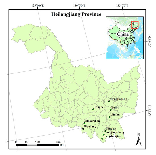
Figure 1.
The distribution of the sampling plots in this study across Heilongjiang province, Northeast China.

Table 1.
Summary statistics of the sample trees in this study.
2.2. Biomass Model
The power function of allometric equations has been commonly used for biomass modeling [10], in which tree biomass is the dependent variable and tree attributes (i.e., DBH and/or H) are the independent or predictor variables [34]. In this study, we applied a likelihood analysis to determine which of the two error structures (additive and multiplicative) was more appropriate to the biomass data of Korean larch [2,35]. It was found that the multiplicative error structure was preferred so that the logarithmic transformation was applied to linearize the power function to construct the linear seemingly unrelated regression (SUR) models. Two additive model systems were constructed in this study as follows:
where , , , and are the biomass of stem, branch, foliage and root, respectively; DBH is the tree diameter at the breast height; H is the tree total height; ln is the natural logarithm; are the model coefficients to be estimated from the data, where the subscript corresponds to the four tree components, and ; and ε is the model error term.
A general expression of linear SUR models (in matrix notation) is
where is a vector of the response variable; is a vector of the error terms; is a matrix of the predictors, including for SURM1, and and for SUMR2; is a vector of the model coefficients; and where is an identity matrix, is the variance–covariance matrix of error term, and is the tensor product, such that:
2.3. Classical Approach of SUR
Generalized least squares (GLS) is an efficient technique for parameter estimation when the error terms between regression models are correlated [2,36]. However, if the covariance of the model errors is unknown, one can get a consistent estimate of using an implementable version of GLS known as the feasible generalized least squares (FGLS). The package systemfit in R software 3.5.3 [37,38] was used to obtain the classical estimations of model coefficients and the covariance matrix in this study.
2.4. Bayesian Approaches of SUR
In Bayesian inference, both model coefficients and covariance are considered random variables with probability distributions that can be calculated using the data D such that
where and are the posterior- and prior-probabilities, respectively, is the likelihood, and the denominator of Equation (5) is the marginal probability of the data D [13]. Based on Equation (5), algorithms of Bayesian approaches were proposed on the SUR models [39]. To implement the Bayesian estimation, we fit the SUR models using both the Gibbs sampler and direct Monte Carlo (DMC) sampling along with different priors [39] (the detailed calculation processes of the Gibbs sampler and DMC are attached in Appendix A).
We proposed five estimations of the SUR models as follows:
- (1)
- Direct Monte Carlo simulation approach using Jeffreys invariant prior (namely DMC).
- (2)
- Gibbs sampler using Jeffreys invariant prior (namely Gs-J).
- (3)
- Gibbs sampler using a multivariate normal distribution with mean vector and variance defined as 0 and 1000 (the covariance is 0) as priors of model parameters, and a default inverted Wishart distribution [25] as the priors of variance–covariance matrix errors (namely Gs-MN), respectively, which was considered as a non-informative prior.
- (4)
- Gibbs sampler using a multivariate normal distribution prior, which consisted of parameters estimated by the FGLS method with subsamples (namely Gs-MN1). The percentages of the subsamples were 10%, 20%, 30%, …, and 90% of the 174 independent trees data, which were sampled without conducting any replacement. Each simulation was repeated 10,000 times.
- (5)
- Gibbs sampler using a prior of multivariate normal distribution, which consisted of the parameters estimated by using logarithmic functions of different biomass components for Larix spp. (namely Gs-MN2). The previous biomass model parameters in the same forms for Larix spp. were collected from a normalized tree biomass equation dataset in Luo et al. [10]. A default inverted Wishart distribution proposed by Rossi and Allenby was used as the prior of variance–covariance matrix errors [25]. Even though the biomass functions were sampled from different areas in China, the model parameters were well represented by a multivariate normal distribution with mean vector and variance–covariance matrix after a multivariate normal test (p > 0.05).
In this study, the FGLS estimates of the model parameters were used as the starting values for the Gs-J method to reach faster convergence and save computational time. For the Gs-MN, Gs-MN1, and Gs-MN2 methods, the starting values were automatically generated in the R package bayesm when the prior distributions were given [40]. On the setting of options for the Gibbs sampler, the size of the posterior samples was set to 33,000, including 3000 burn-in periods and thinning length of 3 to ensure the performance’s stability along with the relatively small autocorrelation of Markov chains constructed. The thinning length of 3 means that we took 1 sample for every 3 samples from the remaining 30,000 samples obtained and subsequently received 10,000 posterior samples. This set of the thinning length is beneficial to reduce the autocorrelations between samples. The convergence of the Gibbs posterior samples was assessed using the Geweke’s and the Heidelberger and Welch’s convergence diagnostic [41,42,43]. For the DMC approach, the process was repeated 10,000 times, corresponding to the Gibbs posterior samples. We used the R package bayesm to implement a Gibbs sampler with a prior multivariate normal distribution [40] and package Coda [43] to conduct the convergence diagnostic. However, there were no published packages that could implement Bayesian analysis with Jeffreys’s prior, and thus we used custom R code to implement the Bayesian estimation of DMC and Gs-J.
2.5. Model Evaluation and Validation
In this study, the deviance information criterion (DIC) was used to evaluate and compare the model fitting of the Bayesian estimations with different priors [28]. In addition, the coefficient of determination () and root mean square error (RMSE) were calculated for the description of model performance [44]. The models with higher and lower DIC and RMSE were preferred.
Model validation is necessary to assess the applicability of the models, because better model fitting does not necessarily indicate better model prediction quality. In this study, we used the leave-one-out cross-validation to test the model prediction performance [45]. Mean absolute error (MAE) and mean absolute percent error (MAE%) were calculated to validate the model prediction performance [2]. The mathematical formula of the DIC, , RMSE, MAE, and MAE% can be expressed as follows:
where is the posterior mean of the deviance (−2 × Log likelihood of the given data and parameters); is the model complexity, which is summarized by the effective number of parameters; and are the observations and predictions, respectively; are the predictions obtained by using leave-one-out cross-validation; and is the sample size.
2.6. Anti-Logarithm Correction Factors
When the logarithmic transformation is applied to the power function, the correction factors (CFs) are commonly used to correct the bias produced by the anti-log transformation. Several CFs from previous studies were compared in this study [2,46,47]:
where is the mean square error and calculated as ; is the sample size; is the number of model parameters; and and are the observations and predictions, respectively, taken from Equations (1) and (2). To compare the effectiveness of the three CFs, three measures were used [2,48,49] as follows:
where is percent bias, is percent standard error, and is mean percentage difference; and represent anti-log observations and anti-log predictions, respectively, by CFs; and is the sample size.
2.7. Stability Analysis for Classical and Bayesian Approaches
Simulations were performed using the subsamples of all biomass data to compare the classical SUR models (FGLS) against the Bayesian SUR models. Specifically, we compared the characteristics of the model parameters and prediction performance using different sample sizes. In the simulation process, we sampled 10, 15, 20, 30, 40, 60, 80, 110, 140, and 170 individuals without replacement from the entire dataset (174 trees), and then the procedure was repeated 5000 times. Within each subsample, we estimated the model parameters using both FGLS and Bayesian estimations. The distributions of estimated parameters were analyzed, and corresponding predictions were summarized and used to calculate the indices of the efficiency of estimation (MAE and MAE%). All simulations were performed using R software 3.5.3 [38].
3. Results
3.1. Fitting the SUR Models
For the Bayesian methods Gs-MN1 on both SURM1 and SURM2, the prior information consisted of the model parameter values estimated by the FGLS method with subsample sizes of 10%, 20%, 30%, …, and 90% of the 174 trees sampled without replacement. For Gs-MN2, the prior information in the normalized tree biomass equation dataset [10] was used to estimate the SURM1 and SURM2 model parameters. The results of statistical tests showed that these derived parameters values indeed followed a multivariate normal distribution. The specific forms and values were as follows:
Gs-MN1 of SURM2:
Gs-MN1 of SURM2:
Gs-MN2 of SURM1:
Gs-MN2 of SURM2:
where in , is the prior mean, and is the prior precision matrix; in , is the degree of freedom parameter for the inverted Wishart prior, and is the scale parameter for the inverted Wishart prior.
The posterior means, standard deviations, and 95% posterior intervals for the Bayesian methods of both SURM1 and SURM2 are reported in Table 2 and Table 3, respectively, in which the posterior draws from the Gibbs sampler successfully passed the convergence test. Furthermore, the parameter estimates and standard errors of FGLS are also listed in Table 2 and Table 3. The means of the posterior draws from different sampling were relatively equal, but there was a significant discrepancy in their standard deviations. The tables indicated that DMC produced the lowest standard deviation, followed by Gs-MN1, Gs-J, Gs-MN2, and Gs-MN, as did the 95% posterior intervals. In order to simplify the comparison, Figure 2 visualizes the results of the posterior draws in the form of probability density plots for the Bayesian methods. The same trend was clearly shown for each model parameter (Figure 2). Furthermore, we calculated the correlation matrix of the model errors between the four tree components after the model parameters were obtained. However, those correlation matrices were not significantly different for the similar parameter estimates between the six modeling methods. Hence, we only illustrated the correlation matrix for DMC in Table A1 (see Appendix B).
Table 2.
The posterior means, standard deviations (std), and 95% posterior intervals (using the 2.5th and 97.5th percentiles of posterior samples) of the SURM1 (DBH-only) parameter estimates, calculated by using the Bayesian estimation. The parameters means and standard errors (SEs) estimated by FGLS are also listed.
Table 3.
The parameter estimates of SURM2 (DBH-H). The symbols are the same as in Table 2.
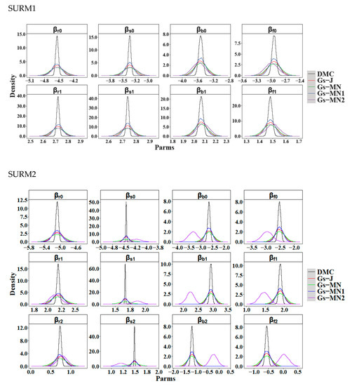
Figure 2.
Posterior distributions of the model parameters estimated by Bayesian statistics. DMC represents the direct Monte Carlo with Jeffreys’ invariant prior; Gs-J is the Gibbs sampler with Jeffreys’ invariant prior; and Gs-MN represents the Gibbs sampler with a prior of multivariate normal distribution by 0 vector, with the corresponding variance of 1000 and the covariance of 0. The Gs-MN1 and Gs-Mn2 is the Gibbs sampler with an informative prior of multivariate normal distribution by different means, variances, and covariances.
3.2. Model Evaluation and Validation
Table 4 presents the , RMSE, and DIC of the six modeling methods for the four tree components (i.e., stem, branch, foliage, and root). According to the DICs, Gs-MN1 performed better than other methods either for SURM1 (DBH as the only predictor) or SURM2 (DBH and H as the predictors). For the non-informative prior Bayesian methods, there was not much difference of DIC between DMC and Gs-J, but there was a significant reduction in DIC for Gs-MN. For the informative priors, only Gs-MN1 produced a relatively better performance in most tree components, while Gs-MN2 performed similarly with other non-informative priors. The results also indicated that all models fitted the larch biomass data well, given all higher than 0.75 in the model (Table 4). The stem biomass models obtained the highest , while the foliage biomass models obtained the smallest . Incorporating H as the second predictor (SUM2) improved the model fitting for the stem, branch, and foliage biomass models, while unexpectedly it resulted in a slight reduction in the model for the root biomass models. In general, the Gs-MN1 method for both SURM1 and SURM2 yielded smaller DIC and relatively similar and RMSE compared with other modeling methods.
Table 4.
The model fitting statistics of the six modeling methods for the four tree biomass components.
The averages and 95% prediction intervals (PIs) for the DBH-only classical method (FGLS), non-informative (DMC, Gs-J, and Gs-MN), and informative priors (Gs-MN1 and Gs-MN2) Bayesian prediction curves are showed in Figure 3. It is clear that the 95% PIs of the five Bayesian methods were much narrower than the FGLS models across all tree components. The results indicate the Bayesian models are more reliable and stable than FGLS. Overall, DMC evidently produced the narrowest 95% PI among the five Bayesian methods, followed by Gs-MN1. On the other hand, the differences between the other three Bayesian methods (i.e., Gs-J, Gs-MN, Gs-MN2) were indistinguishable.
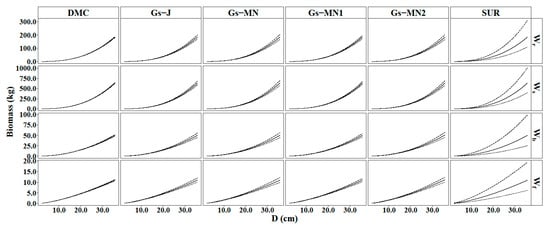
Figure 3.
The 95% prediction interval of Wr, Ws, Wb, and Wf predictions from the six approaches.
Leave-one-out cross-validation was used to validate the log-transformed SUR models for the six methods (Table 5). According to MAE and MAE%, the model prediction bias varied across different tree components. The stem and branch models consistently produced the smallest and the largest MAE%, respectively, across all methods for both SURM1 and SURM2, while Gs-MN1 yielded the best prediction for both SUM1 and SUM2 for most tree components (Table 5).
Table 5.
The model validation statistics of six modeling methods for the four tree biomass components.
3.3. Comparison of Correction Factors on Anti-Log Transformation
In order to further analyze the effects of applying different correction factors, the percent bias (B, %) and percent standard error (G, %) of three correction factors (CF1, CF2, and CF3) for both SURM1 and SURM2 were calculated using the Gs-MN1 method (Table 5). In addition, the mean percentage difference (MPD, %) of CF0, CF1, CF2, and CF3 was also listed in Table 6 (CF0 = 1, without applying any correction factor). Surprisingly, SURM2 always had smaller values of correction factors (B, G, and MPD) across the four tree components than those of SURM1, indicating that adding H into the biomass equations indeed improved the model fitting and performance. However, the values of the correction factors, B, and G were relatively similar for the CF1, CF2, and CF3, revealing that the three correction factors were indistinguishable for either SURM1 or SURM2 in this study. Further, the mean percentage difference of the uncorrected prediction (MPD0) was the lowest value (Table 6), so that the correction factor might not be necessary for the anti-log transformation in this study.
Table 6.
The percent bias (B, %) and percent standard error (G, %) of the three correction factors (CF1, CF2, and CF3) with the mean percentage difference (MPD, %) of the CF0, CF1, CF2, and CF3 calculated by the error terms obtained using the Gs-MN1. MPD0 was calculated without using any correction factor (CF0), in which CF0 = 1.
3.4. Stability Analysis in Repeated Trials between Various Sizes of Data and Methods
In this study, the parameter estimates obtained by FGLS and Bayesian methods were similar using the entire biomass data (Table 2 and Table 3). However, the two methods produced the parameter estimates with different ranges when the sample size decreased, in which the FGLS models had a wider range of the parameter estimates than those of the Bayesian models on SURM1 (Figure 4), in which the five models (except Gs-J) were selected to illustrate the stability of the parameter estimation methods. Figure A1 (see Appendix B) shows the trend of SURM2, which is similar to that of SURM1. It was evident that the ranges of the parameter estimates decreased as the subsample size increased. The distributions of the parameter estimates were relatively identical for each subsample size in DMC and FGLS, in which both methods estimated the parameters outside the confidence intervals obtained with the entire data (174 trees). For the other non-informative priors, the simulation results of Gs-MN were slightly different from both DMC and FGLS. The Bayesian methods with the informative priors produced less variation or fluctuation for the parameter estimates with narrower ranges than those with the non-informative priors (Figure 4 and Figure 5). For the small subsamples of Gs-MN2, the means of the parameter estimates clearly deviated from the means of the parameter estimates obtained with the entire data, while Gs-MN1 performed well in each subsample size. The results indicated that using an inaccurate informative prior will produce incorrect results.
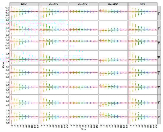
Figure 4.
Simulation results for the parameters estimation of SURM1 using the DMC, Gs-MN, Gs-MN1, Gs-MN2, and FGLS. The dashed and solid horizontal lines represent the 95% confidence intervals and means of the simulation using the entire dataset (174 trees), respectively.
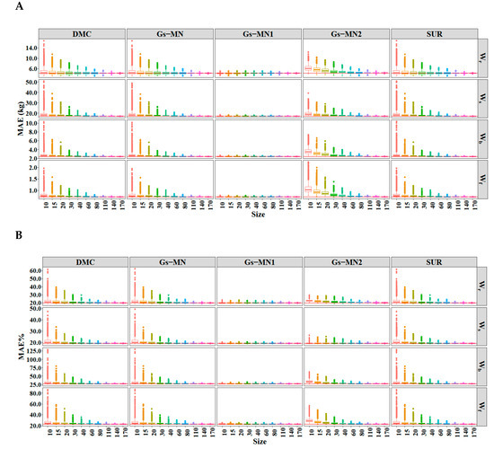
Figure 5.
The (A) and (B) of the SURM1 using different sample sizes. Solid horizontal line represents the value of MAE and MAE% calculated using the entire dataset (174 trees).
The MAEs and MAE%s were calculated using SURM1 produced in the simulations and reapplied to the entire data (Figure 5); the simulation result of SURM2 was highly similar to that of SURM1, as shown in Figure A2 (see Appendix B). The summary of MAEs and MAE%s for all methods and tree components across ten different sample sizes are given in Table A2 (see Appendix B). SURM2 had a higher prediction efficiency than SURM1 from the values of the MAEs and MAE%s. Further, the prediction bias of Gs-MN1 was most stable, indicating that a good informative prior has the advantages of using a small number of data. For Gs-MN2, the prediction bias calculated using the parameter estimates obtained from the small samples deviated significantly from those calculated using all data, although the ranges of MAE and MAE% were smaller than both Bayesian models with non-informative priors and FGLS.
4. Discussion
4.1. Biomass SUR Models
Tree biomass is the basis for estimating net primary production and carbon of forest ecosystems, especially when the global carbon emissions and carbon sinks have gradually become the emergent topics [50,51]. Usually, allometric equations are used to develop tree biomass models for specific species and areas [8,14]. In our research, two additive model systems (i.e., SURM1 and SURM2) were constructed to estimate tree biomass of planted Korean larch by both classical and Bayesian approaches. The main objective of this study was to explore the advantages of Bayesian approaches on the SUR biomass models of the four tree components (i.e., stem, branch, foliage, and root). As we expected, our results demonstrated that applying the Bayesian methods on the SUR model systems not only obtained better model fitting and predictions, but also provided the assessment and evaluation of the uncertainties for constructing and updating tree biomass models.
For computational efficiency, we compared the computing time for both FGLS and Bayesian approaches on the SURM1 estimations by a computer of a 3.2 GHz Intel (R) Core (TM) i7—8700 CPU and RAM of 32.0 GB. The result showed that it took about 0.46 s to obtain the posterior samples of parameters for the Bayesian approaches (i.e., Gs-MN, Gs-MN1 and Gs-MN2) when the sample size was 33,000 (including 3000 burn-in periods and 3 thinning length) using the R package bayesm, while the classical FGLS took only 0.03 s to get the parameter estimates using the R package systemfit. It was clear that the computing time of both approaches was small enough to be ignored. However, the DMC and Gs-J took more time (about 15 min) to estimate the models of the same setup described above, which may be caused by the limitation of our customized R codes, and the computation would have been faster if the codes had been optimized.
The published research revealed that the model parameters of biomass equations can be described by a multivariate normal distribution. In other words, the variability in these model parameters represented different biotic and abiotic factors influencing its own allometric biomass relationships for specific species and locations [13]. With the Bayesian approaches, the model parameters of new locations can be estimated and updated from the prior information, which was different from the calibration of the random-effect parameters in mixed-effect models [14], because the random-effect parameters were fixed for a specific level. Compared to the classical approaches, the Bayesian approaches produced narrower 95% prediction intervals so that the Bayesian statistics have the advantages of reducing uncertainty and obtaining more stable predictions (Figure 3) [13,32], and the good prior information improved the accuracy of biomass predictions (Table 5). However, the Bayesian approaches sometimes performed worse if the prior information was not good, like Gs-MN2.
Our results of stability analysis showed the evidence, as we expected, that the Bayesian approaches with informative priors provided more stable parameter estimates and reduced the uncertainty of parameters for small sample sizes, similar to the findings of Zapatacuartas et al. [13] (also see more discussion in the Section 4.2). The smaller fluctuations of both MAE and MAE% for the Bayesian methods with the informative priors indicated that the Bayesian methods had higher estimation efficiency than the classical method, especially for small sample sizes (N = 10, 20, 30). However, the difference in the estimation efficiency between FGLS and Bayesian methods decreased as the sample size increased. Overall, the sample size reflected the amount of the prior data information, of which the values of the posterior parameters mainly depended [28,30]. Increasing sample size continuously corrected the prior distribution until it significantly improved the posterior distribution. This phenomenon can be considered as one of the reasons that the estimations of non-informative Bayesian and FGLS were identical.
Considering the inherent correlations between tree components (additivity or compatibility) in developing biomass equations has been recognized as an essential characteristic of the biomass model systems [2,4]. Numerous SUR models in the literature commonly used one or even more constraints in the simultaneous model fitting process [18,52]. Zhao et al. [53], Dong et al. [14], and Widagdo et al. [54] conducted a comprehensive simulation and comparison of applying zero, one, and three restriction(s) in the SUR model systems. All of these researches confirmed that applying SUR without using any constraint, as proposed by Affleck and Diéguez-Aranda [55], gave slightly better model predictions than those using one or more constraints. Therefore, we decided to use no constraint to account for the correlations between tree components. Our results indicated that the correlation coefficients ranged from 0.1062 to 0.5836 across the tree components for SURM1, while they were slightly smaller (from 0.0026 to 0.5432) for SURM2. Therefore, it was appropriate to jointly fit the simultaneous biomass equations.
The sole DBH predictor of the SUR model (SURM1) produced relatively large variations for the tree components, and the inclusion of H as the second predictor variable in stem, branch, and foliage biomass models (SURM2) yielded a relatively greater enhancement on the model performance for both model fitting and validation. Our results were compatible with previous publications [8,56]. Further analyses showed that the root biomass model’s performance using DBH as the sole predictor was better than those of two predictors (DBH and H), although the parameter estimates of H were statistically significant. These findings indicated that the benefit of adding H as the additional predictor on root biomass models was relatively small [56,57]. Overall, SURM2 apparently produced better parameter estimation and model prediction than SURM1 for three of the four tree components biomass.
4.2. Non-Informative vs. Informative Priors in Bayesian Methods
Both DMC and Gs-J used the Jeffreys non-informative priors but obtained slightly different results for model fitting. The DIC values indicated that DMC was better than Gs-J, with smaller standard deviations (Table 2 and Table 3, and Figure 2). The Gs-J method needed to check on the posterior samples’ convergence, while DMC did not. Zellner [39] reported one of the advantages of DMC, in which DMC might generate independent samples within a weak autocorrelation. Hence, we also evaluated the posterior samples’ autocorrelation of the parameter βr0 (Table A3 in Appendix B). The autocorrelation of various methods at every non-zero lag was very small, indicating that the autocorrelation in the posterior samples rarely existed. Thus, it may not be apparent that the DMC’s autocorrelation was less than those of other methods based on the Gibbs sampler, which was slightly different from Zellner’s inference [39]. As described in Section 2.4, the thinning length used in the Gibbs sampler’s posterior samples was set to 3 in order to weaken the autocorrelation, but this step was absent in Zellner [39].
The DMC method seemed to be more efficient in the computation process according to the real size of the generated posterior samples (DMC method was 10,000 and Gibbs was 33,000), similar to the inferences in other studies [58]. However, the computational efficiency may not become the future’s primary indicator in evaluating the quality of the estimation method, since computing capacity has been exponentially increased over the years. Furthermore, the Gs-MN method also used a non-informative prior of multivariate normal distribution with mean vector 0 and variance 1000 (covariance is 0), in which its standard deviations of the model parameters were larger than Gs-J. This phenomenon may be caused by the variances of model parameters in the priors being set to 1000. When the variances were limited, there was still an upper and lower limit, although the distribution range of the prior’s parameters was relatively wide. Thus, this can be categorized as a pseudo-non-informative prior with remarkably insufficient information.
In our study, we determined two types of informative priors according to the samples’ sources to further implement the Gibbs sampler-based Bayesian analysis. The first type was derived from the results of our data’s repeated self-sampling (Gs-MN1), while the other was acquired from the literature (Gs-MN2). The self-sampling informative prior gave a more accurate value of not only parameters’ means and variances, but also fitting and validation performance compared with the one based on the literature’s informative prior. These findings confirmed that accurate informative priors would bring a greater improvement in the model performances. Overall, the Gs-MN1 method produced the smallest DIC value, followed sequentially by DMC, Gs-J, Gs-MN, and Gs-MN2. However, our results also suggested that, at least by using the data obtained from this research, the literature’s informative priors may not be suitable for biomass modeling in the study area. In future research, further research on the determination of prior information is still needed to improve biomass model performance.
4.3. Anti-Logarithm Correction Factor
Logarithmic transformation in biomass modeling is used to simply linearize the nonlinear relationships between biomass and predictors [59,60]. It is important to make a decision on whether or not a bias correction is needed. Usually, it is determined by the size of the error term [61]. In this study, three evaluated correction factors (CFs) were all small (ranging from 1.0058 to 1.0604). For the statistics of CFs, the B and G were relatively similar, suggesting that the difference between the CFs was not significant. Furthermore, we also compared the mean percentage difference (MPD) of the four types of CFs (CF0, CF1, CF2, and CF3). The results showed that MPD0 (calculated by CF0) was the smallest among others, indicating that the anti-log correction may not be necessary for our biomass data. In general, the CFs’ inferences obtained in this study were consistent with previous research [61,62].
5. Conclusions
In this study, we applied Bayesian methods to construct two sets of the seemingly unrelated regression models (i.e., SURM1 and SURM2) with no constraint to take account of the inherent correlations between four tree components (i.e., stem, branch, foliage, and root) collected from the same tree. The classical method FGLS was also used to estimate the model parameters of the SUR models as comparison. The Bayesian methods with the informative priors not only produced better model fitting, but also higher prediction accuracy and computing efficiency. In addition, the Bayesian methods had more stable predictions for small sample sizes, which could be used to estimate new model parameters in new locations, as we suggested. However, finding good informative priors for the model parameters was crucial and necessary to improve the model fitting and prediction accuracy and efficiency. On the other hand, the anti-logarithm correction factors on the model predictions may not be necessary for our developed models, as the model error terms were relatively small.
Overall, applying the Bayesian methods on the SUR models of tree biomass showed good benefits compared to the classical modeling method, especially when the amount of available data was relatively small. These newly-developed SUR models based on Bayesian methods can be used to accurately estimate the tree biomass of planted Korean larch in northeast China and to estimate carbon storage and further understand the energy matter distribution of larch plantations.
Author Contributions
L.D. and F.L. provided the data, conceived the ideas, and designed methodology; L.X. analyzed the data and wrote the manuscript. F.R.A.W. and L.Z. helped in analyzing the data and writing the paper. All authors contributed critically to the data collection and manuscript preparation. All authors have read and agreed to the published version of the manuscript.
Funding
This research was financially supported by the National Natural Science Foundation of China (No. 31971649), the National Key R&D Program of China (No. 2017YFD0600402), Provincial Funding for National Key R&D Program of China in Heilongjiang Province (No. GX18B041), the Fundamental Research Funds for the Central Universities (No. 2572019CP08) and the Heilongjiang Touyan Innovation Team Program (Technology Development Team for High-Efficient Silviculture of Forest Resources).
Acknowledgments
The authors would like to thank the faculty and students of the Department of Forest Management, Northeast Forestry University (NEFU), China, who provided and collected the data for this study. And the authors also thank two anonymous reviewers for suggestions and comments that improved the contents and quality of the manuscript.
Conflicts of Interest
The authors declare no conflict of interest.
Appendix A
Classical Approach of SUR
A m-dimensional linear SUR model system can be expressed as follows:
where , and are . A general expression of linear SUR models (in matrix notation) is
FGLS for estimating SUR model system:
Step 1. Fit the m linear functions of the SUR models individually and calculate the error terms for each function, where ;
Step 2. Compute the variance–covariance matrix of obtained in step 1 by Equation (A3):
Step 3. Estimate the model coefficients by GLS as follows:
where upper right T is a transpose of the matrix, and is the variance–covariance matrix.
Bayesian approaches of SUR
Based on Equation (A2), the likelihood function by giving the data D is
Gibbs Sampler on SUR models
- A simple prior of and was expressed as follows:where denotes the multivariate normal distribution, where is the prior mean vector of , and is the number of parameters in the single model of Equation (A1); is the prior precision matrix of ; and denotes the inverse Wishart distribution, where both and are the degree of freedom and prior precision matrix for the inverse Wishart prior. The normal prior of is conjugated with the conditional likelihood of Equation (A5), and the posterior of by giving is normal:where and . Meanwhile, the inverted Wishart prior is a conditional conjugate and is used to obtain the posterior distribution with the following prior:where is the matrix of , and in Equation (A1).
- A non-informative prior that is widely used, namely Jeffreys invariant prior is expressed as follows:The conditional posteriors are [39]where , and .
According to the conditional posteriors on Equations (A7), (A8), (A10), and (A11), a Markov Chain Monte Carlo (MCMC) method with a Gibbs sampler can be used to obtain posterior samples of the SUR model parameters. The steps of the Gibbs sampler on SUR models are summarized as follows:
- Step 1.
- Give the starting values of , namely , the starting values were obtained from prior distributions generally;
- Step 2.
- Draw from Equation (A7) or (A10);
- Step 3.
- Draw from Equation (A8) or (A11);
- Step 4.
- Repeat both step 2 and step 3 to draw and for N times, ,
where N is the sample size that could be manually set.
DMC for estimating SUR model system
The SUR models (Equation (A1)) are reformulated as follows:
with , , and . There is no correlation detected between the error terms and of Equation (A12). The is the design matrix that including predictors, and is the vector of model parameters, where =1, 2, 3 and 4. Thus, the likelihood function of the data D becomes
Herein, we set the Jeffreys invariant prior as the prior:
then the conditional normal inverse-gamma posterior is
The sampling procedure of m-dimensional SUR models can be determined using the following steps:
- Step 1. Set to generate (), where N is the samples size. Draw from the Equation (A15).
- Step 2. is set as the increment, and then is drawn by using Equation (A16) to generate the in Equation (A15).
- Step 3. Repeat the step 2 sequentially until is reached.
- Step 4. Transform into to .
The more detailed information of DMC approach could be found in the Zellner’s inference [39].
Predicting with Bayesian method
Given the posterior samples of model parameters, the predictive density of model’s dependent variables can be approximated as follows:
Appendix B

Figure A1.
Simulation results for the parameter estimations of SURM2 using the DMC, Gs-MN, Gs-MN1, Gs-MN2, and FGLS. The dashed and solid horizontal lines represent the 95% confidence intervals and means of the simulation using the entire dataset (174 trees), respectively.

Figure A2.
The (A) and (B) of the SURM2 using different sample sizes. The solid line represents the value of MAE and MAE% calculated by all dataset (174 trees).
Table A1.
The correlation matrices of SURM1 and SURM2 fitted by DMC method.
Table A1.
The correlation matrices of SURM1 and SURM2 fitted by DMC method.
| Model | Correlation Matrix | ||||
|---|---|---|---|---|---|
| SURM1 | |||||
| 1.0000 | −0.4292 | −0.2428 | 0.4487 | ||
| −0.4292 | 1.0000 | 0.5836 | −0.2208 | ||
| −0.2428 | 0.5836 | 1.0000 | −0.1062 | ||
| 0.4487 | −0.2208 | −0.1062 | 1.0000 | ||
| SUMR2 | |||||
| 1.0000 | 0.0026 | 0.0084 | 0.2311 | ||
| 0.0026 | 1.0000 | 0.5342 | −0.0362 | ||
| 0.0084 | 0.5342 | 1.0000 | 0.0042 | ||
| 0.2311 | −0.0362 | 0.0042 | 1.0000 | ||
Table A2.
The average of the mean absolute error (, kg) and average of the mean absolute percent error ( ) of the six modeling methods with different sample sizes in the simulations for the four tree biomass components.
Table A2.
The average of the mean absolute error (, kg) and average of the mean absolute percent error ( ) of the six modeling methods with different sample sizes in the simulations for the four tree biomass components.
| Methods | Components | Indices | Sample Sizes | |||||||||
|---|---|---|---|---|---|---|---|---|---|---|---|---|
| 10 | 15 | 20 | 30 | 40 | 60 | 80 | 110 | 140 | 170 | |||
| SUM1 | ||||||||||||
| DMC | Wr | 4.89 | 4.62 | 4.50 | 4.42 | 4.38 | 4.37 | 4.37 | 4.36 | 4.36 | 4.37 | |
| 22.08 | 21.23 | 20.86 | 20.50 | 20.32 | 20.16 | 20.07 | 20.01 | 19.98 | 19.97 | |||
| Ws | 19.36 | 18.48 | 18.14 | 17.80 | 17.63 | 17.47 | 17.39 | 17.31 | 17.28 | 17.27 | ||
| 21.16 | 20.41 | 20.09 | 19.79 | 19.64 | 19.50 | 19.43 | 19.38 | 19.36 | 19.34 | |||
| Wb | 2.80 | 2.66 | 2.59 | 2.53 | 2.49 | 2.46 | 2.45 | 2.43 | 2.43 | 2.42 | ||
| 31.94 | 30.16 | 29.35 | 28.59 | 28.25 | 27.90 | 27.74 | 27.60 | 27.51 | 27.47 | |||
| Wf | . | 0.81 | 0.77 | 0.76 | 0.75 | 0.74 | 0.73 | 0.73 | 0.73 | 0.72 | 0.72 | |
| 26.62 | 25.12 | 24.50 | 23.91 | 23.64 | 23.35 | 23.23 | 23.13 | 23.06 | 23.02 | |||
| Gs-MN | Wr | 4.90 | 4.63 | 4.51 | 4.42 | 4.39 | 4.37 | 4.37 | 4.36 | 4.36 | 4.36 | |
| 22.09 | 21.24 | 20.87 | 20.50 | 20.33 | 20.15 | 20.08 | 20.02 | 19.98 | 19.97 | |||
| Ws | 19.33 | 18.47 | 18.14 | 17.80 | 17.63 | 17.47 | 17.39 | 17.32 | 17.28 | 17.27 | ||
| 21.14 | 20.41 | 20.09 | 19.79 | 19.64 | 19.50 | 19.43 | 19.38 | 19.35 | 19.34 | |||
| Wb | 2.80 | 2.66 | 2.59 | 2.53 | 2.49 | 2.46 | 2.45 | 2.43 | 2.43 | 2.42 | ||
| 31.97 | 30.18 | 29.36 | 28.59 | 28.25 | 27.89 | 27.73 | 27.59 | 27.52 | 27.47 | |||
| Wf | 0.81 | 0.77 | 0.76 | 0.75 | 0.74 | 0.73 | 0.73 | 0.73 | 0.72 | 0.72 | ||
| 26.63 | 25.13 | 24.51 | 23.92 | 23.64 | 23.37 | 23.24 | 23.13 | 23.06 | 23.02 | |||
| Gs-MN1 | Wr | 4.30 | 4.31 | 4.32 | 4.33 | 4.33 | 4.34 | 4.35 | 4.35 | 4.35 | 4.36 | |
| 19.89 | 19.92 | 19.95 | 19.97 | 19.98 | 19.97 | 19.96 | 19.95 | 19.95 | 19.95 | |||
| Ws | 17.28 | 17.28 | 17.28 | 17.29 | 17.29 | 17.28 | 17.28 | 17.27 | 17.27 | 17.26 | ||
| 19.37 | 19.37 | 19.38 | 19.38 | 19.37 | 19.36 | 19.36 | 19.35 | 19.34 | 19.34 | |||
| Wb | 2.43 | 2.43 | 2.43 | 2.43 | 2.43 | 2.43 | 2.43 | 2.42 | 2.42 | 2.42 | ||
| 27.65 | 27.65 | 27.65 | 27.62 | 27.61 | 27.59 | 27.57 | 27.53 | 27.49 | 27.47 | |||
| Wf | 0.72 | 0.72 | 0.72 | 0.72 | 0.72 | 0.72 | 0.72 | 0.72 | 0.72 | 0.72 | ||
| 23.17 | 23.17 | 23.17 | 23.15 | 23.14 | 23.12 | 23.10 | 23.07 | 23.04 | 23.02 | |||
| Gs-MN2 | Wr | 6.28 | 5.73 | 5.37 | 4.98 | 4.78 | 4.60 | 4.53 | 4.47 | 4.44 | 4.43 | |
| 22.72 | 22.10 | 21.66 | 21.10 | 20.79 | 20.46 | 20.29 | 20.17 | 20.10 | 20.07 | |||
| Ws | 19.76 | 18.91 | 18.45 | 17.99 | 17.78 | 17.57 | 17.47 | 17.37 | 17.33 | 17.30 | ||
| 19.54 | 19.51 | 19.51 | 19.49 | 19.48 | 19.42 | 19.39 | 19.36 | 19.34 | 19.33 | |||
| Wb | 3.60 | 3.19 | 2.96 | 2.73 | 2.62 | 2.53 | 2.49 | 2.46 | 2.45 | 2.44 | ||
| 34.22 | 31.79 | 30.50 | 29.18 | 28.58 | 28.05 | 27.82 | 27.64 | 27.53 | 27.48 | |||
| Wf | 1.08 | 0.96 | 0.89 | 0.81 | 0.78 | 0.75 | 0.74 | 0.73 | 0.73 | 0.73 | ||
| 29.76 | 27.16 | 25.62 | 24.23 | 23.69 | 23.32 | 23.19 | 23.10 | 23.03 | 22.99 | |||
| FGLS | Wr | 4.89 | 4.62 | 4.50 | 4.42 | 4.38 | 4.36 | 4.37 | 4.36 | 4.36 | 4.36 | |
| 22.08 | 21.23 | 20.86 | 20.50 | 20.32 | 20.15 | 20.08 | 20.02 | 19.98 | 19.97 | |||
| Ws | 19.36 | 18.48 | 18.14 | 17.80 | 17.63 | 17.47 | 17.39 | 17.32 | 17.28 | 17.27 | ||
| 21.16 | 20.41 | 20.09 | 19.79 | 19.64 | 19.50 | 19.43 | 19.38 | 19.35 | 19.34 | |||
| Wb | 2.80 | 2.66 | 2.59 | 2.53 | 2.49 | 2.46 | 2.45 | 2.43 | 2.43 | 2.42 | ||
| 31.94 | 30.16 | 29.35 | 28.59 | 28.25 | 27.89 | 27.73 | 27.59 | 27.52 | 27.47 | |||
| Wf | 0.81 | 0.77 | 0.76 | 0.75 | 0.74 | 0.73 | 0.73 | 0.73 | 0.72 | 0.72 | ||
| 26.61 | 25.12 | 24.50 | 23.91 | 23.64 | 23.37 | 23.24 | 23.13 | 23.06 | 23.02 | |||
| SURM2 | ||||||||||||
| DMC | Wr | 5.18 | 4.76 | 4.61 | 4.46 | 4.40 | 4.34 | 4.31 | 4.28 | 4.27 | 4.27 | |
| 21.67 | 20.14 | 19.55 | 18.97 | 18.71 | 18.41 | 18.26 | 18.15 | 18.09 | 18.04 | |||
| Ws | 9.49 | 8.88 | 8.60 | 8.33 | 8.20 | 8.08 | 8.02 | 7.96 | 7.93 | 7.91 | ||
| 10.05 | 9.39 | 9.10 | 8.83 | 8.70 | 8.57 | 8.50 | 8.45 | 8.41 | 8.38 | |||
| Wb | 2.72 | 2.53 | 2.45 | 2.37 | 2.33 | 2.29 | 2.27 | 2.26 | 2.26 | 2.25 | ||
| 29.39 | 27.21 | 26.34 | 25.38 | 24.97 | 24.56 | 24.38 | 24.23 | 24.11 | 24.05 | |||
| Wf | 0.86 | 0.80 | 0.78 | 0.76 | 0.75 | 0.74 | 0.74 | 0.73 | 0.73 | 0.73 | ||
| 27.61 | 25.49 | 24.63 | 23.80 | 23.47 | 23.15 | 23.02 | 22.94 | 22.88 | 22.86 | |||
| Gs-MN | Wr | 5.16 | 4.76 | 4.61 | 4.46 | 4.40 | 4.34 | 4.31 | 4.28 | 4.27 | 4.27 | |
| 21.62 | 20.13 | 19.55 | 18.97 | 18.71 | 18.41 | 18.26 | 18.15 | 18.09 | 18.04 | |||
| Ws | 9.49 | 8.88 | 8.60 | 8.33 | 8.20 | 8.08 | 8.02 | 7.96 | 7.93 | 7.91 | ||
| 10.05 | 9.39 | 9.11 | 8.83 | 8.70 | 8.57 | 8.51 | 8.45 | 8.41 | 8.38 | |||
| Wb | 2.70 | 2.53 | 2.45 | 2.37 | 2.33 | 2.29 | 2.27 | 2.26 | 2.26 | 2.25 | ||
| 29.34 | 27.21 | 26.34 | 25.38 | 24.97 | 24.56 | 24.38 | 24.23 | 24.11 | 24.05 | |||
| Wf | 0.85 | 0.80 | 0.78 | 0.76 | 0.75 | 0.74 | 0.74 | 0.73 | 0.73 | 0.73 | ||
| 27.57 | 25.49 | 24.63 | 23.80 | 23.47 | 23.15 | 23.02 | 22.94 | 22.88 | 22.86 | |||
| Gs-MN1 | Wr | 4.24 | 4.25 | 4.25 | 4.26 | 4.26 | 4.26 | 4.26 | 4.26 | 4.26 | 4.26 | |
| 18.07 | 18.09 | 18.11 | 18.12 | 18.13 | 18.11 | 18.09 | 18.07 | 18.05 | 18.02 | |||
| Ws | 7.96 | 7.96 | 7.96 | 7.96 | 7.96 | 7.95 | 7.94 | 7.93 | 7.92 | 7.91 | ||
| 8.44 | 8.45 | 8.45 | 8.45 | 8.45 | 8.44 | 8.43 | 8.41 | 8.40 | 8.38 | |||
| Wb | 2.26 | 2.26 | 2.26 | 2.26 | 2.26 | 2.26 | 2.26 | 2.26 | 2.25 | 2.25 | ||
| 24.30 | 24.30 | 24.31 | 24.28 | 24.26 | 24.22 | 24.19 | 24.14 | 24.08 | 24.05 | |||
| Wf | 0.73 | 0.73 | 0.73 | 0.73 | 0.73 | 0.73 | 0.73 | 0.73 | 0.73 | 0.73 | ||
| 22.98 | 22.98 | 22.98 | 22.97 | 22.96 | 22.94 | 22.92 | 22.90 | 22.88 | 22.87 | |||
| Gs-MN2 | Wr | 6.45 | 6.04 | 5.67 | 5.18 | 4.92 | 4.67 | 4.55 | 4.47 | 4.41 | 4.38 | |
| 24.50 | 22.72 | 21.52 | 20.10 | 19.41 | 18.82 | 18.57 | 18.39 | 18.29 | 18.21 | |||
| Ws | 13.68 | 12.59 | 11.71 | 10.59 | 10.02 | 9.48 | 9.17 | 8.85 | 8.62 | 8.46 | ||
| 14.08 | 12.97 | 12.14 | 11.15 | 10.69 | 10.25 | 9.98 | 9.65 | 9.38 | 9.17 | |||
| Wb | 3.47 | 3.30 | 3.19 | 3.05 | 2.95 | 2.78 | 2.65 | 2.49 | 2.38 | 2.32 | ||
| 36.87 | 35.73 | 35.04 | 33.87 | 32.94 | 31.31 | 29.94 | 28.24 | 26.97 | 26.11 | |||
| Wf | 1.08 | 0.97 | 0.91 | 0.85 | 0.82 | 0.78 | 0.76 | 0.75 | 0.73 | 0.72 | ||
| 30.93 | 28.73 | 27.60 | 26.49 | 25.86 | 25.04 | 24.47 | 23.84 | 23.40 | 23.10 | |||
| FGLS | Wr | 5.18 | 4.76 | 4.61 | 4.46 | 4.40 | 4.34 | 4.31 | 4.28 | 4.27 | 4.27 | |
| 21.67 | 20.14 | 19.55 | 18.97 | 18.71 | 18.41 | 18.26 | 18.15 | 18.09 | 18.04 | |||
| Ws | 9.49 | 8.88 | 8.60 | 8.33 | 8.20 | 8.08 | 8.02 | 7.96 | 7.93 | 7.91 | ||
| 10.05 | 9.39 | 9.10 | 8.83 | 8.70 | 8.57 | 8.50 | 8.45 | 8.41 | 8.38 | |||
| Wb | 2.72 | 2.53 | 2.45 | 2.37 | 2.33 | 2.29 | 2.27 | 2.26 | 2.26 | 2.25 | ||
| 29.39 | 27.21 | 26.34 | 25.38 | 24.97 | 24.56 | 24.38 | 24.23 | 24.11 | 24.05 | |||
| Wf | 0.86 | 0.80 | 0.78 | 0.76 | 0.75 | 0.74 | 0.74 | 0.73 | 0.73 | 0.73 | ||
| 27.61 | 25.49 | 24.63 | 23.80 | 23.47 | 23.15 | 23.02 | 22.94 | 22.88 | 22.86 | |||
Table A3.
The autocorrelation function of the posterior samples for the parameter βr0 of the Bayesian methods calculated using 10,000 samples. The max lag was set to 50.
Table A3.
The autocorrelation function of the posterior samples for the parameter βr0 of the Bayesian methods calculated using 10,000 samples. The max lag was set to 50.
| Lag | DMC | Gs-J | Gs-MN | Gs-MN1 | Gs-MN2 |
|---|---|---|---|---|---|
| SURM1 | |||||
| 0 | 1.0000 | 1.0000 | 1.0000 | 1.0000 | 1.0000 |
| 1 | −0.0005 | 0.0120 | −0.0060 | 0.0033 | 0.0062 |
| 5 | −0.0108 | 0.0059 | 0.0296 | 0.0078 | 0.0002 |
| 10 | 0.0149 | −0.0011 | −0.0043 | −0.0180 | −0.0011 |
| 50 | −0.0020 | −0.0011 | 0.0075 | 0.0015 | 0.0160 |
| SURM2 | |||||
| 0 | 1.0000 | 1.0000 | 1.0000 | 1.0000 | 1.0000 |
| 1 | 0.0022 | −0.0039 | 0.0051 | 0.0007 | −0.0040 |
| 5 | −0.0104 | 0.0001 | 0.0037 | −0.0048 | −0.0181 |
| 10 | 0.0033 | −0.0087 | −0.0048 | 0.0021 | −0.0057 |
| 50 | −0.0018 | 0.0014 | 0.0043 | −0.0108 | −0.0129 |
where the subscript means the new data that need to be predicted, and is the matrix of new independent variables; and are the parameters and variance–covariance matrix of errors, respectively; and is the size of the posterior samples.
References
- Clark, J.; Murphy, G. Estimating forest biomass components with hemispherical photography for Douglas-fir stands in northwest Oregon. Can. J. For. Res. 2011, 41, 1060–1074. [Google Scholar] [CrossRef]
- Dong, L.; Zhang, L.; Li, F. A compatible system of biomass equations for three conifer species in Northeast, China. For. Ecol. Manag. 2014, 329, 306–317. [Google Scholar] [CrossRef]
- Weiskittel, A.R.; MacFarlane, D.W.; Radtke, P.J.; Affleck, D.L.; Hailemariam, T.; Woodall, C.W.; Westfall, J.A.; Coulston, J.W. A call to improve methods for estimating tree biomass for regional and national assessments. J. For. 2015, 113, 414–424. [Google Scholar] [CrossRef]
- Zhao, D.; Kane, M.; Markewitz, D.; Teskey, R.; Clutter, M. Additive tree biomass equations for midrotation Loblolly pine plantations. For. Sci. 2015, 61, 613–623. [Google Scholar] [CrossRef]
- Ter-Mikaelian, M.T.; Korzukhin, M.D. Biomass equations for sixty-five north American tree species. For. Ecol. Manag. 1997, 97, 1–24. [Google Scholar] [CrossRef]
- Jenkins, J.C.; Chojnacky, D.C.; Heath, L.S.; Birdsey, R.A. National-scale biomass estimators for united states tree species. For. Sci. 2003, 49, 12–35. [Google Scholar]
- Zianis, D.; Muukkonen, P.; Makipaa, R.; Mencuccini, M. Biomass and stem volume equations for tree species in Europe. Silva Fenn. Monogr. 2005, 4, 63. [Google Scholar]
- Wang, C. Biomass allometric equations for 10 co-occurring tree species in Chinese temperate forests. For. Ecol. Manag. 2006, 222, 9–16. [Google Scholar] [CrossRef]
- Chave, J.; Rejoumechain, M.; Burquez, A.; Chidumayo, E.N.; Colgan, M.S.; Delitti, W.B.C.; Duque, A.; Eid, T.; Fearnside, P.M.; Goodman, R.C. Improved allometric models to estimate the aboveground biomass of tropical trees. Glob. Chang. Biol. 2014, 20, 3177–3190. [Google Scholar] [CrossRef]
- Luo, Y.; Wang, X.; Ouyang, Z.; Lu, F.; Feng, L.; Tao, J. A review of biomass equations for China’s tree species. Earth Syst. Sci. Data 2020, 12, 21–40. [Google Scholar] [CrossRef]
- Bi, H.; Murphy, S.; Volkova, L.; Weston, C.J.; Fairman, T.A.; Li, Y.; Law, R.; Norris, J.; Lei, X.; Caccamo, G. Additive biomass equations based on complete weighing of sample trees for open eucalypt forest species in south-eastern Australia. For. Ecol. Manag. 2015, 349, 106–121. [Google Scholar] [CrossRef]
- Kralicek, K.; Huy, B.; Poudel, K.P.; Temesgen, H.; Salas, C. Simultaneous estimation of above- and below-ground biomass in tropical forests of Viet Nam. For. Ecol. Manag. 2017, 390, 147–156. [Google Scholar] [CrossRef]
- Zapatacuartas, M.; Sierra, C.A.; Alleman, L. Probability distribution of allometric coefficients and Bayesian estimation of aboveground tree biomass. For. Ecol. Manag. 2012, 277, 173–179. [Google Scholar] [CrossRef]
- Dong, L.; Zhang, Y.; Xie, L.; Li, F. Comparison of tree biomass modeling approaches for larch (Larix olgensis Henry) trees in Northeast China. Forests 2020, 11, 202. [Google Scholar] [CrossRef]
- Parresol, B.R. Assessing tree and stand biomass: A review with examples and critical comparisons. For. Sci. 1999, 45, 573–593. [Google Scholar]
- Zellner, A. An efficient method of estimating seemingly unrelated regressions and tests for aggregation bias. J. Am. Stat. Assoc. 1962, 57, 348–368. [Google Scholar] [CrossRef]
- Mehtätalo, L.; Lappi, J. Biometry for Forestry and Environmental Data: With Examples in R; Chapman and Hall; CRC Press: New York, NY, USA, 2020; p. 426. [Google Scholar]
- Dong, L.; Zhang, L.; Li, F. Additive biomass equations based on different dendrometric variables for two dominant species (Larix gmelini Rupr. and Betula platyphylla Suk.) in natural forests in the Eastern Daxing’an Mountains, Northeast China. Forests 2018, 9, 261. [Google Scholar] [CrossRef]
- Parresol, B.R. Additivity of nonlinear biomass equations. Can. J. For. Res. 2001, 31, 865–878. [Google Scholar] [CrossRef]
- Zellner, A. An Introduction to Bayesian Inference in Econometrics; Wiley: New York, NY, USA, 1971; p. 448. [Google Scholar]
- Lu, L.; Wang, H.; Chhin, S.; Duan, A.; Zhang, J.; Zhang, X. A Bayesian model averaging approach for modelling tree mortality in relation to site, competition and climatic factors for Chinese fir plantations. For. Ecol. Manag. 2019, 440, 169–177. [Google Scholar] [CrossRef]
- Griffiffiths, W.E. Bayesian Inference in the Seemingly Unrelated Regressions Model; Department of Economics, The University of Melbourne: Melbourne, Australia, 2003; p. 520. [Google Scholar]
- Bayes, T. An essay towards solving a problem in the doctrine of chances. M.D. Comput. 1991, 8, 157. [Google Scholar] [CrossRef]
- Li, R.; Stewart, B.; Weiskittel, A.R. A Bayesian approach for modelling non-linear longitudinal/hierarchical data with random effects in forestry. Forestry 2012, 85, 17–25. [Google Scholar] [CrossRef]
- Rossi, P.E.; Allenby, G.M. Bayesian Statistics and Marketing; John Wiley & Sons, Ltd.: Chichester, UK, 2005; p. 368. [Google Scholar]
- Huelsenbeck, J.P.; Ronquist, F.; Nielsen, R.; Bollback, J.P. Bayesian inference of phylogeny and its impact on evolutionary biology. Science 2001, 294, 2310–2314. [Google Scholar] [CrossRef] [PubMed]
- Portinale, L.; Raiteri, D.C.; Montani, S. Supporting reliability engineers in exploiting the power of dynamic Bayesian networks. Int. J. Approx. Reason. 2010, 51, 179–195. [Google Scholar] [CrossRef]
- Reich, B.J.; Ghosh, S.K. Bayesian Statistical Methods; CRC Press: Boca Raton, FL, USA, 2019; p. 275. [Google Scholar]
- Berger, J.O. Bayesian analysis: A look at today and thoughts of tomorrow. J. Am. Stat. Assoc. 2000, 95, 1269–1276. [Google Scholar] [CrossRef]
- Samuel, K.; Wu, X. Modern Bayesian Statistics; China Statistics Press: Beijing, China, 2000; p. 244.
- Van Ravenzwaaij, D.; Cassey, P.; Brown, S.D. A simple introduction to Markov Chain Monte–Carlo sampling. Psychon. Bull. Rev. 2018, 25, 143–154. [Google Scholar] [CrossRef]
- Zhang, X.; Duan, A.; Zhang, J. Tree biomass estimation of Chinese fir (Cunninghamia lanceolata) based on Bayesian method. PLoS ONE 2013, 8, e79868. [Google Scholar] [CrossRef]
- State Forestry and Grassland Administration The Ninth Forest Resource Survey Report (2014–2018); China Forestry Press: Beijing, China, 2018; p. 451.
- Zeng, W.; Duo, H.; Lei, X.; Chen, X.; Wang, X.; Pu, Y.; Zou, W. Individual tree biomass equations and growth models sensitive to climate variables for Larix spp. in China. Eur. J. For. Res. 2017, 136, 233–249. [Google Scholar] [CrossRef]
- Xiao, X.; White, E.P.; Hooten, M.B.; Durham, S.L. On the use of log-transformation vs. nonlinear regression for analyzing biological power laws. Ecology 2011, 92, 1887–1894. [Google Scholar] [CrossRef]
- SAS Institute Inc. SAS/ETS® 14.1 User’s Guide; SAS Institute Inc.: Cary, NC, USA, 2015; p. 4100. [Google Scholar]
- Henningsen, A.; Hamann, J.D. Systemfit: A package for estimating systems of simultaneous equations in R. J. Stat. Softw. 2007, 23, 1–40. [Google Scholar] [CrossRef]
- R Core Team. R: A Language and Environment for Statistical Computing; R Foundation for Statistical Computing: Vienna, Austria, 2019. [Google Scholar]
- Zellner, A.; Ando, T. A direct Monte Carlo approach for Bayesian analysis of the seemingly unrelated regression model. J. Econom. 2010, 159, 33–45. [Google Scholar] [CrossRef]
- Rossi, P. Bayesm: Bayesian Inference for Marketing/Micro-Econometrics; R package version 3.1-4. 2019. Available online: https://CRAN.R-project.org/package=bayesm (accessed on 20 April 2020).
- Heidelberger, P.; Welch, P.D. Simulation run length control in the presence of an initial transient. Oper. Res. 1983, 31, 1109–1144. [Google Scholar] [CrossRef]
- Gewke, J. Evaluating the accuracy of sampling-based approaches to calculating posterior moments. In Bayesian Statistics 4; Bernado, J.M., Berger, J.O., Dawid, A.P., Smith, A.F.M., Eds.; Clarendon Press: Oxford, UK, 1992; pp. 169–193. [Google Scholar]
- Plummer, M.; Best, N.; Cowles, K.; Vines, K. Coda: Convergence diagnosis and output analysis for MCMC. R News 2006, 6, 7–11. [Google Scholar]
- Fu, L.; Sharma, R.P.; Hao, K.; Tang, S. A generalized interregional nonlinear mixed-effects crown width model for prince rupprecht larch in northern China. For. Ecol. Manag. 2017, 389, 364–373. [Google Scholar] [CrossRef]
- Cawley, G.C.; Talbot, N.L.C. Efficient leave-one-out cross-validation of kernel fisher discriminant classifiers. Pattern Recognit. 2003, 36, 2585–2592. [Google Scholar] [CrossRef]
- Finney, D.J. On the distribution of a variate whose logarithm is normally distributed. J. R. Statist. Soc. B 1941, 7, 155–161. [Google Scholar] [CrossRef]
- Baskerville, G.L. Use of logarithmic regression in the estimation of plant biomass. Can. J. For. Res. 1972, 4, 149. [Google Scholar] [CrossRef]
- Wiant, H.V.; Harner, E.J. Percent bias and standard error in logarithmic regression. For. Sci. 1979, 25, 167–168. [Google Scholar]
- Yandle, D.O.; Wiant, H.V. Estimation of plant biomass based on the allometric equation. Can. J. For. Res. 1981, 11, 833–834. [Google Scholar] [CrossRef]
- Bond-Lamberty, B.; Wang, C.; Gower, S.T. Net primary production and net ecosystem production of a boreal black spruce wildfire chronosequence. Glob. Chang. Biol. 2004, 10, 473–487. [Google Scholar] [CrossRef]
- Pregitzer, K.S.; Euskirchen, E.S. Carbon cycling and storage in world forests: Biome patterns related to forest age. Glob. Chang. Biol. 2004, 10, 2052–2077. [Google Scholar] [CrossRef]
- Wang, X.; Zhao, D.; Liu, G.; Yang, C.; Teskey, R.O. Additive tree biomass equations for Betula platyphylla Suk. plantations in Northeast China. Ann. For. Sci. 2018, 75, 60. [Google Scholar] [CrossRef]
- Zhao, D.; Westfall, J.A.; Coulston, J.W.; Lynch, T.B.; Bullock, B.P.; Montes, C.R. Additive biomass equations for slash pine trees: Comparing three modeling approaches. Can. J. For. Res. 2019, 49, 27–40. [Google Scholar] [CrossRef]
- Widagdo, F.R.A.; Li, F.; Zhang, L.; Dong, L. Aggregated biomass model systems and carbon concentration variations for tree carbon quantification of natural Mongolian Oak in Northeast China. Forests 2020, 11, 397. [Google Scholar] [CrossRef]
- Affleck, D.L.R.; Dieguez-Aranda, U. Additive nonlinear biomass equations: A likelihood-based approach. For. Sci. 2016, 62, 129–140. [Google Scholar] [CrossRef]
- Dong, L.; Zhang, L.; Li, F. Developing additive systems of biomass equations for nine hardwood species in Northeast China. Trees-Struct. Funct. 2015, 29, 1149–1163. [Google Scholar] [CrossRef]
- Kusmana, C.; Hidayat, T.; Tiryana, T.; Rusdiana, O. Istomo Allometric models for above- and below-ground biomass of Sonneratia spp. Glob. Ecol. Conserv. 2018, 15, 10. [Google Scholar]
- Ando, T. Bayesian variable selection for the seemingly unrelated regression models with a large number of predictors. J. Jpn. Stat. Soc. 2012, 41, 187–203. [Google Scholar] [CrossRef]
- Tang, S. Bias correction in logarithmic regression and comparison with weighted regression for non-linear models. For. Res. 2011, 24, 137–143. [Google Scholar]
- Mascaro, J.; Litton, C.M.; Hughes, R.F.; Uowolo, A.; Schnitzer, S.A. Is logarithmic transformation necessary in allometry? Ten, one--hundred, one--thousand--times yes. Biol. J. Linn. Soc. 2014, 111, 230–233. [Google Scholar] [CrossRef]
- Madgwick, H.A.I.; Satoo, T. On estimating the aboveground weights of tree stands. Ecology 1975, 56, 1446–1450. [Google Scholar] [CrossRef]
- Zianis, D.; Xanthopoulos, G.; Kalabokidis, K.; Kazakis, G.; Ghosn, D.; Roussou, O. Allometric equations for aboveground biomass estimation by size class for Pinus brutia Ten. trees growing in North and South Aegean Islands, Greece. Eur. J. For. Res. 2011, 130, 145–160. [Google Scholar] [CrossRef]
Publisher’s Note: MDPI stays neutral with regard to jurisdictional claims in published maps and institutional affiliations. |
© 2020 by the authors. Licensee MDPI, Basel, Switzerland. This article is an open access article distributed under the terms and conditions of the Creative Commons Attribution (CC BY) license (http://creativecommons.org/licenses/by/4.0/).