Allometric Equations for Shrub and Short-Stature Tree Aboveground Biomass within Boreal Ecosystems of Northwestern Canada

Abstract

Aboveground biomass (AGB) of short-stature shrubs and trees contain a substantial part of the total carbon pool within boreal ecosystems. These ecosystems, however, are changing rapidly due to climate-mediated atmospheric changes, with overall observed decline in woody plant AGB in boreal northwestern Canada. Allometric equations provide a means to quantify woody plant AGB and are useful to understand aboveground carbon stocks as well as changes through time in unmanaged boreal ecosystems. In this paper, we provide allometric equations, regression coefficients, and error statistics to quantify total AGB of shrubs and short-stature trees. We provide species- and genus-specific as well as multispecies allometric models for shrub and tree species commonly found in northwestern boreal forest and peatland ecosystems. We found that the three-dimensional field variable (volume) provided the most accurate prediction of shrub multispecies AGB (R² = 0.79, p < 0.001), as opposed to the commonly used one-dimensional variable (basal diameter) measured on the longest and thickest stem (R² = 0.23, p < 0.001). Short-stature tree AGB was most accurately predicted by stem diameter measured at 0.3 m along the stem length (R² = 0.99, p < 0.001) rather than stem length (R² = 0.29, p < 0.001). Via the two-dimensional variable cross-sectional area, small-stature shrub AGB was combined with small-stature tree AGB within one single allometric model (R² = 0.78, p < 0.001). The AGB models provided in this paper will improve our understanding of shrub and tree AGB within rapidly changing boreal environments.

1. Introduction

Ecosystems in northwestern Canada are changing rapidly due to a warming climate, drier conditions, extended growing season, and climate-mediated increases in frequency and intensity of disturbances, such as wildfire, permafrost thaw, insect and pathogen outbreaks, and anthropogenic natural resource extraction (e.g., [1,2,3]). One of the significant outcomes of climate-mediated change in these environments is the increased abundance of short-stature vegetation, such as shrubs [4,5] and low productive and juvenile trees, in particular where wildfire disturbance sets back ecosystems to an early successional stage post fire [4] or in the rapidly changing transition zones between elevated forests and adjacent peatlands due to permafrost thaw [6]. Increased shrub cover influences important ecosystem functions, such as energy balance and hydrology [6] at local to regional scales and greenhouse gas/carbon–climate cycle feedbacks at national to global scales [6,7], which could ultimately exacerbate these changes [8,9]. Shrubs and short-stature trees contain a substantial part of the total aboveground carbon of unmanaged boreal forest and peatland ecosystems, although specific numbers remain uncertain [10]. For quantification of the complete carbon balance of Canada, aboveground biomass (AGB) of shrubs and short-stature trees need to be integrated into carbon accounting strategies in the future.

Although shrubification in permafrost environments has been reported [5,8,11,12,13], spatially explicit quantities of shrub and short-stature tree AGB remain largely unknown for boreal northwestern Canada for three reasons: (a) Existing allometric models for plant species were developed for larger tree individuals harvested in managed forests for merchantable volume [14,15]. As such, these models are not appropriate for quantification of the AGB of short-stature shrubs and trees growing in unmanaged ecosystems. (b) There is a lack of regionally applicable allometric models for shrub and short-stature tree species for unmanaged forests in boreal northwestern Canada. He et al. [16] provide regression coefficients for allometric equations developed for three common shrub species and genera. However, these local models were developed for shrubs growing in two different peatland sites located in a different ecozone and as such may be less accurate when applied in a different study region within the discontinuous to sporadic permafrost zone and a different ecosystem type, such as transition zones between forest and peatlands. (c) The best predictor variable to model AGB of small-stature shrubs and trees remains unknown. Existing boreal shrub allometric equations typically use a 1D field variable, e.g., basal stem diameter [11,16,17,18], to predict the mass of a 3D object (the shrub). However, the applicability of these models for scaling from a 1D variable to a 3D quantity has not been evaluated for shrubs and short-stature trees.

Here, we test the applicability of 1D, 2D, and 3D field measurements within allometric models to understand and improve the scaling relationships across shrub and short-stature tree species up to 4.5 m in height (herein “tree species”) in northern boreal regions. 1D field measurements describe shrub and tree structures based on a single-length observation, such as diameter or stem length. 2D field measurements, such as cross-sectional area, represent two directions, while 3D measurements describe plant structures in three different directions (x, y, and z), such as volume.

The objectives of this study were as follows: (a) develop regional allometric models using 1D, 2D, and 3D field measurements to predict aboveground biomass of shrubs and short-stature trees (herein “trees”); (b) compare the utility of scaling using 1D, 2D, and 3D field-based models for all shrubs and all tree species combined (a general equation, which may be of utility for active remote sensing applications, such as lidar, in the future); (c) provide allometric models for total AGB for each shrub and each tree species and genus examined as well as for the pooled data; and (d) recommend optimal methods of field data collection for prediction of shrub and small-stature tree AGB. We hypothesized that 3D field variables would be best suited to predict shrub AGB because a 3D measurement considers the 3D properties of the plant structure. We also hypothesized that, by pooling data, the results would be less accurate; however, doing so would allow us to include these measures within a remote sensing-based structural model of biomass (e.g., using airborne lidar).

2. Materials and Methods

2.1. Study Area

Shrub and tree species examined in this study were destructively sampled across the southern margin of the sporadic to discontinuous permafrost zone of the Taiga Plains and Taiga Shield ecozones (Figure 1). The mean annual air temperature varies from −2.5 (Fort Simpson, Taiga Plains) to between −3 and −4 (Yellowknife, Taiga Shield) °C, while cumulative annual precipitation is 390 (Fort Simpson) and 360 (Yellowknife) mm, respectively [19,20].

The geology is dominated by lacustrine plains overlain by peatlands with fine- to coarse-textured lacustrine and till in the mid-boreal Taiga Plains, which transitions towards the high boreal Taiga Shield into nearly level to rolling and hilly bedrock [19,20]. In the Taiga Plains, approximately 25%–50% of the land surface area is covered by peatlands, consisting of peat plateaus underlain by permafrost, bogs, and fens [21]. While shrubs dominantly grow in the transition zones between peat plateaus and bogs or fens, short-stature trees grow within upland forests or on elevated peat plateaus. In the high-boreal Taiga Shield, peatlands cover an area of less than 5% and occupy hollows within and between bedrock exposures [20]. The dominant vegetation in the mid-boreal Taiga Plains consists of black spruce (Picea mariana) and mixed hardwood and softwood forests containing similar species as found in the Taiga Shield ecozone. Taiga Shield ecosystems are dominated by black spruce and jack pine (Pinus banksiana) with abundance of paper birch (Betula papyrifera) and trembling aspen (Populus tremuloides) [19,20].

2.2. Shrub Measurements, Destructive Sampling, and Processing

To determine AGB of small-stature shrubs and trees growing in the mid-boreal Taiga Plains and high-boreal Taiga Shield ecoregions, we derived allometric models for five common shrub genera and species (Alnus spp., Betula spp., Dasiphora fruticosa, Salix spp., and Shepherdia canadensis) and four common tree genera and species (Betula papyrifera, Picea spp., Populus balsamifera, and Populus tremuloides). Plant individuals were measured and destructively sampled within 65 peatlands and upland forest ecosystems distributed across the two ecoregions in late July/early August 2018 and 2019. Field sample locations were situated in late successional sites and in sites disturbed by wildland fire within the last 50 years (Figure 1,

Table 1. Overview of aboveground biomass (AGB) of shrub and tree samples harvested per ecoregion.

Ecozone	Transects (Samples)
Shrub Samples
Taiga Plains	31 (127)
Taiga Shield	15 (79)
Tree Samples
Taiga Plains	20 (105)
Total	66 (311)

) in order to represent the high variability of boreal ecosystem disturbance by wildfire and permafrost thaw in our allometric models.

Harvested plants were located within <10 m of field transects (Figure 2a), which were set up randomly within each site. Between one to three transects were installed per site. Field transects were 25 m in length, starting in upland forests and traversing into peatlands and crossing the forest–peatland transition zone perpendicularly. This setup was chosen in order to capture the shrub abundance within the transition zones between peat plateaus and bogs/fens, where the largest and fastest ecosystem changes have been observed [6]. Shrubs were located along the transect with distance from the start of the transect. Shrubs were selected per transect within standing height ranges of 0.5 up to 3.5 m. A shrub individual was selected when it was alive and mostly free of leaf or stem disturbances. Up to five shrub individuals were sampled per transect.

Measured 1D variables for each individual shrub sample included maximum height (herein “max height” (m)), average maximum height (m), number of individual stems, and basal diameter of each stem (cm). Heights were measured using a tape measure, and diameters were measured with a caliper. Previous studies have examined the relationship between the AGB of a single stem and the 1D independent variable measurement of the same stem [11,16]. However, boreal shrubs are commonly multi-stemmed. In order to analyze how accurately 1D field-measured variables from a single stem can predict the AGB of the entire plant, we tested the basal diameter of the stem with the widest diameter (herein “max basal diameter” (cm)) and the length of the longest stem (herein “max stem length” (m)) within allometric relationships. To test a 2D variable, we transformed each basal diameter to cross-sectional area (cm²) and summed this to total cross-sectional area per shrub individual. For the 3D variable, we measured the extent of the uppermost foliage layer perpendicular to the transect (herein “width” (m)) and parallel to the transect (herein “line-intercept cover” (m)) using a tape measure. The 3D shrub volume (m³) (1) was then calculated as follows:

Volume (m³) = max height (m) × line-intercept cover (m) × width (m).

(1)

Following measurements in situ, shrubs were clipped directly above the soil surface (Figure 2c) and stored in paper bags for further processing. Dead stems were not harvested. In the laboratory, harvested samples were air dried for up to four months, separated into stem and leaf parts, and oven dried at 60 °C for 48 h [22]. Twigs and fruits were included as leaf parts. The total AGB was determined as dry weight (g) by weighing each shrub part (woody and leafy) and summing the dry weight of all parts per shrub individual.

2.3. Tree Measurements, Sampling, and Processing

Small-stature tree AGB was collected in late July 2019 along 20 random transects adjacent to the permanent sample plots set up by the Canadian Forest Service, located near Fort Liard, Northwest Territories (NWT), Canada. Live trees were chosen from the understory and open areas across different height ranges determined in intervals of 0.5 m up to ≤4.5 m. In all cases, samples were mostly free of foliage disturbance/mortality and stem blemishes. In situ 1D tree measurements included stem length (m), and stem diameter (cm) measured at 0.03, 0.15, 0.30, and 1.3 m along the stem length starting from the average ground surface surrounding the tree. Stem diameters were transformed to cross-sectional area (cm²) per tree individual to provide a 2D variable analogous to that for shrubs and thus offer the potential for a joint shrub and juvenile/low productive tree allometric equation. 3D volume was not measured for trees because tree AGB can best be predicted with diameter, stem length, or both variables combined (e.g., [14]). Following measurements in situ, trees were cut as close to the ground surface as possible and packed into large paper bags to be transported back to the University of Lethbridge. In the laboratory, trees were separated into stem, branch, and leaf components after air drying of up to four months. Branches were cut off directly at the stem. Twigs and fruits were included as leaf parts, while bark was included as part of the stem. Dead branches were not included in the analysis. Oven drying and biomass derivation was completed using the methods described above for shrubs.

2.4. Derivation of Aboveground Biomass Allometric Equations

In situ structural measurements of harvested shrubs and trees were used to determine the most accurate 1D, 2D, or 3D independent variables to predict AGB. Three different forms of single variable regression analysis, which are most commonly used in biomass allometry [11,16,17,23,24,25] were tested for each 1D, 2D, and 3D independent variable per shrub and tree genus and species and for the pooled data. These were used to determine the most descriptive regression model of AGB for genus/species, multispecies shrubs, and multispecies trees as well as in general for all trees and shrubs combined. The first allometric biomass model (2) uses linear regression of the log-transformed dependent $\left(y\right)$ and independent in situ $\left(x\right)$ variables (herein “linear logarithmic regression (LLR)”):

$$\ln \left(y\right)=\ln \left(\beta \right)+\alpha \ast \ln \left(x\right)$$

(2)

where $\alpha$ and $\beta$ are the regression coefficients. The back-transformation to an arithmetic scale was achieved using Equation (3):

$$y =\beta x^{\alpha }$$

(3)

However, the back-transformation resulted in a skewed distribution of $\widehat{y}$ [23]. Baskerville [23] reported a general underestimation of 10%–20% when back-transforming the logarithmic regression estimates of AGB without correcting for skewness. To set this into context, we compared the results of LLR with the results of linear logarithmic regression with correction (herein “LLRC”) (4–6):

$$\mathit{ln}\left(y\right) = \mathit{ln}\left(\beta \right)+\alpha \ast \mathit{ln}\left(x\right)+\mathit{ln}\left(\epsilon \right)$$

(4)

$$y =\beta x^{\alpha }\ast \epsilon$$

(5)

$$\epsilon =e^{\left(\frac{\mathrm{MSE}}{2}\right)}$$

(6)

where $\epsilon$ represents a multiplicative correction factor of the back-transformation with $\mathrm{MSE}$ as the mean square error of the regression [23,25]. This correction removes the bias in Equation (3), which occurs following the back-transformation from a normal distribution of $\ln \left(\widehat{y}\right)$ for a given $\ln \left(x\right)$. LLR results are presented only to set LLRC model results into context, and usage is not recommended without the provided correction factor.

To avoid the problem of skewness, a majority of the research on biomass allometry have used the untransformed nonlinear relationship between dependent and independent variables to predict tree [17] and shrub [11,16,17] AGB. These models use iterative nonlinear least squares regression via a power function (herein “nonlinear least squares regression (NLS)”) with an additive error term $\epsilon$:

$$y =\beta x^{\alpha }$$

(7)

The NLS function for biomass prediction is available in statistical software packages (e.g., “nls” function in the “stats” package in R [26]). The default nonlinear equation that is implemented in R assumes a homogeneous variance of regression residuals [25]. However, trees and shrubs can be inherently heteroscedastic, such that the assumption of homogeneous residual variance across the range of the independent variable could lead to biased model predictions [25]. Although weights can be specified in NLS functions, these should be applied when both arithmetic and logarithmic variances do not show uniformity [23]. Our AGB data showed uniform variances on arithmetic scales for most species and on logarithmic scales for all species. To understand the performance of using a non-weighted nonlinear model that does not address potential heteroscedasticity within the data, we compared NLS (7) with the results of the logarithmic-based models LLR (2–3) and LLRC (4–6).

The modeled biomass results of these three allometric models were evaluated using root mean square error (RMSE), coefficient of determination (R²), and regression residual analysis. Residual analysis was performed using visual inspection of the relationships between dependent and independent variables as well as the total percentage error (%) derived via (8):

$$Total percentage error = \frac{{{\displaystyle \sum }}^{}Modeled AGB-{{\displaystyle \sum }}^{}Measured AGB}{{{\displaystyle \sum }}^{}Measured AGB}\ast 100$$

(8)

Significance of the differences between the genus/species-specific AGB model means and the multispecies model means were evaluated with the t-test for equal variances and Welch’s t-test for unequal variances. Equality of variances was tested with the F-test.

2.5. Biomass Allometric Models

In total, we used 1D, 2D, and 3D input variables and three different forms of regression (LLR, LLRC, and NLS) to predict shrub AGB. Regression coefficients and standard errors were calculated for (a) total shrub AGB per genus/species; (b) all shrubs combined per ecoregion; and (c) all shrubs within both ecoregions combined. Here, (c) represents a multispecies shrub allometric equation that can be applied to all shrubs across the southern half of the study region (NWT, Canada; Figure 1). For short-stature trees, we examined 1D and 2D predictor variables (3D tree volume predictors were not measured) and the three different regression equations described above (LLR, LLRC, and NLS). Similar to shrubs, we have provided the allometric models that most accurately predict (a) total AGB for each tree species; (b) all tree species combined per ecoregion; and (c) for all trees within the two ecoregions combined (herein “multispecies trees”). In addition to individual “shrub” and “tree” models, we have provided a 2D input variable allometric model for total AGB prediction for small-stature shrubs and trees combined (herein “general shrubs and trees”). With the “general shrub and tree” model, we explored the utility of a single 1D (stem length) or 2D (cross-sectional area) variable for combined shrub and tree AGB prediction to understand whether these variables scale uniformly between shrubs and trees. Such combined approaches may have utility for rapid assessment in the field or using less invasive observation techniques (e.g., unmanned airborne vehicles or laser scanning) where vegetation species and type may be indeterminate.

3. Results and Discussion

The ranges and averages (± standard deviation) of the predictor variables for 205 shrubs and 106 trees are provided in Supplementary Material 1, Tables S1 and S2, respectively. Regression coefficients, correction factors, and standard errors are presented in Supplementary Material 2, Tables S3–S5, and can be input into Equations (2)–(7). For all allometric models, regression coefficients were positive, indicating increasing biomass with increasing predictor variable for total AGB, as was found by Lambert et al. [14].

The applicability of multispecies models to predict total AGB for single genus and species has been shown for shrubs by He et al. [16]. Similarly, the differences between our modeled means of total AGB via the multispecies equations and the genus/species-specific modeled means were not significant (p > 0.05). Furthermore, the difference between the modeled means of shrub and tree biomass in previously burned sites and the unburned sites was not significant (p > 0.05). Species-specific coefficients for input into the allometric Equations (2)–(7) are provided in Supplementary Material 2, Table S3, using volume as the predictor and Supplementary Material 2, Table S4, using cross-sectional area as the predictor.

3.1. Comparison of 1D, 2D, and 3D Variables for Shrub Total AGB Prediction

For the genus/species-specific 1D-based models using max stem length or max basal diameter as input into each of the three allometric models (LLR, LLRC, and NLS), Betula spp., Dasiphora fruticosa, and Salix spp. had lower R² (0.005 ≤ R² ≤ 0.325) compared to Shepherdia canadensis (0.433 ≤ R² ≤ 0.809, Table S6). 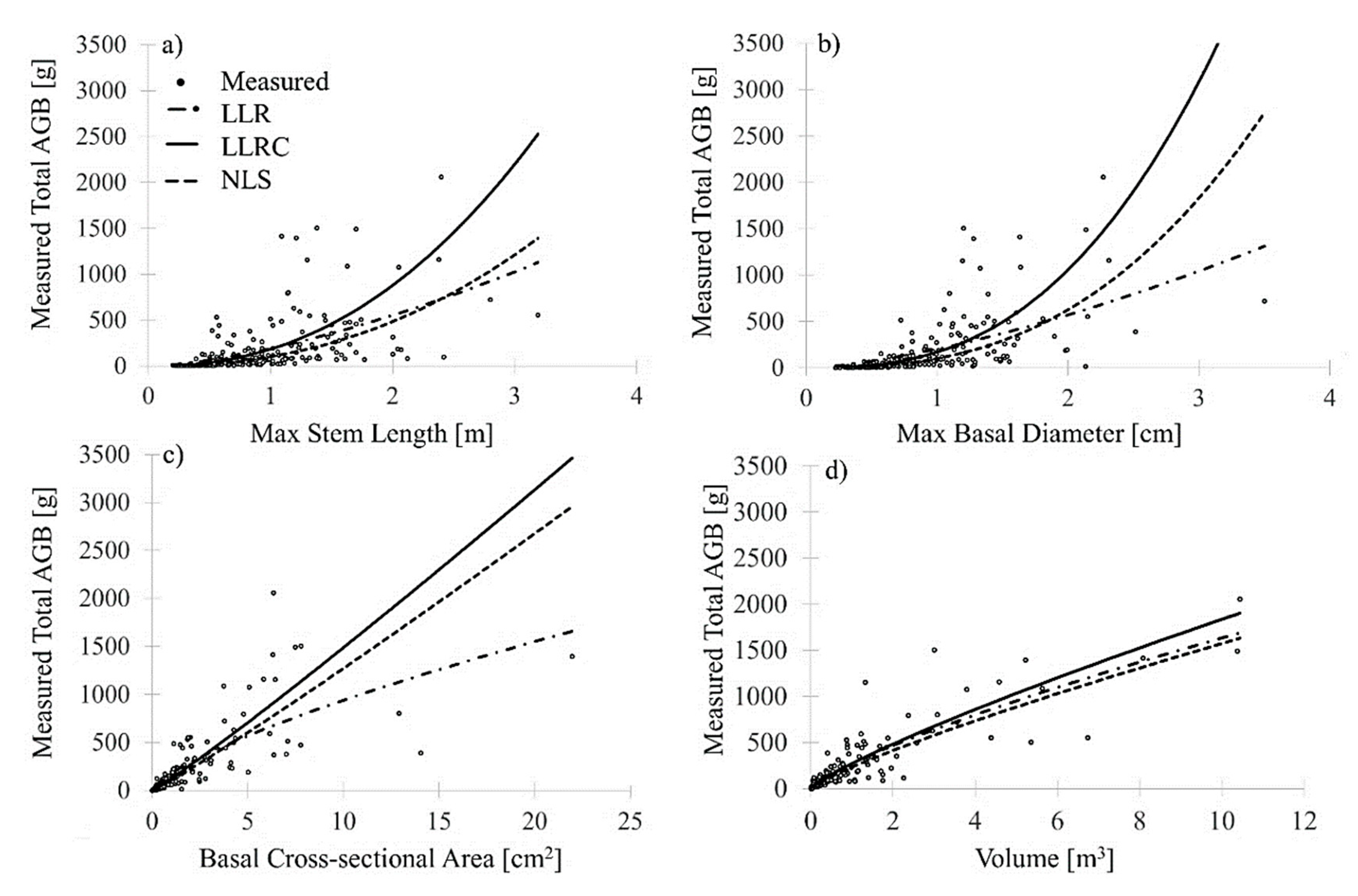In addition, Dasiphora fruticosa was the only species where stem length was not significantly related (p > 0.05) to the dependent variable of measured total AGB. For the multispecies shrub models (pooled for all shrub genera and species), the use of 1D predictor variables yielded the lowest model fits (RMSE) ranging from 262 (NLS) to 318 (LLRC) g for max stem length and 252 (NLS) to 388 (LRC) g for max basal diameter (

Table 2. Model performances for multispecies shrub total ABG prediction (all p values < 0.001).

Model	Dimension	Input Variable	Total Percentage Error (%)	RMSE (g)	R2
Linear logarithmic regression (LLR)	1D	Max stem length	−32	276.12	0.237
	1D	Max basal Diameter	−26	293.20	0.228
	2D	Cross-sectional Area basal	−4	233.46	0.534
	3D	Volume	−11	144.08	0.788
Linear logarithmic regression with correction (LLRC)	1D	Max stem length	23	317.95	0.237
	1D	Max basal Diameter	24	388.00	0.228
	2D	Cross-sectional Area basal	13	263.55	0.534
	3D	Volume	4	144.12	0.788
Nonlinear least squares regression (NLS)	1D	Max stem length	4	262.22	0.273
	1D	Max basal Diameter	8	251.68	0.335
	2D	Cross-sectional Area basal	10	190.75	0.621
	3D	Volume	1	141.04	0.790

). These results are in contrast with previous allometric models for boreal [11,16,17] or subtropical [27] shrubs, where the 1D variable basal diameter of the longest stem had provided the most accurate prediction of total AGB. However, 1D field variables, although related to the dependent variable (p < 0.001) (with the exception of max stem length of Dasiphora fruticosa), did not explain total AGB variability when considering all stems of the entire plant (0.228 ≤R² ≤ 0.335, Table 2, Figure 3a,b). This was true for each genus/species model as well as the multispecies equation, with the exception of Sheperdia canadensis. For this species, max basal diameter was a similarly good predictor variable (R² = 0.809) to cross-sectional area (R² = 0.738) and volume (R² = 0.765, Table S6). The performance of total AGB models increased for all other genera and species as well as for all genera and species combined using the 3D predictor variable of volume, with R² ranging between 0.684 (Betula spp. and Dasiphora fruticosa) and 0.882 (Alnus spp.). The RMSEs for the multispecies models ranged from 141 (NLS) to 144 (LLR and LLRC) g with R² of ~0.790 using any of the three models (LLR, LLRC, and NLS; Table 2). Figure 3a–d shows the relationship between the three models for 1D, 2D, and 3D variables for the multispecies shrub AGB.

Of the three model forms tested, the 3D volume predictor produced the most consistent shrub AGB results (Figure 3,

Table 3. Regression coefficients for each 1D, 2D, and 3D model to predict total AGB for multispecies shrubs with LLRC and NLS.

	Variable	LLRC β	NLS β	LLRC α	NLS α
Multispecies shrubs	Max stem length	100.988	192.186	2.262	1.530
	Max basal diameter	100.484	203.796	2.642	1.486
	Cross-sectional area	106.911	177.614	1.075	0.723
	Volume	233.224	272.116	0.829	0.778

), suggesting the choice of model form is less critical when using a 3D predictor. As expected, the exponent $\alpha$ was greater for 1D models and close to unity for the 3D models. This suggests that a simple linear model would result in similar model fits compared to the LLRC or NLS models when using a 3D predictor. However, after testing this (results not shown), the model results achieved slightly less goodness of fit (R² = 0.769, RMSE 148.6 g) compared to LLRC or NLS (Table 2). Decreasing exponents (holding all else equal) can be explained by the nature of allometric scaling between 1D, 2D, and 3D measurements of a plant to its mass (a 3D attribute) via a power function. Assuming no change in the multiplier (β) (which might be considered analogous to a density attribute), scaling from a 1D measurement to a 3D property requires a higher exponent (α) compared to scaling from a 2D or 3D measurement (Table 3). Therefore, predictions that are extrapolated from lower to higher dimensions contain more inherent model-based uncertainty than predictions requiring no dimensional extrapolation. However, field volume observations consisted of three single measurements and therefore might contain a high overall measurement uncertainty compared to a single 1D measurement. The exact quantity of model vs. field measurement error propagation is unknown, but the net outcome of the tests performed shows that 3D volume produced the highest AGB model accuracies, followed by 2D and then 1D models.

Better model performance and linearity via the 3D predictor variable of volume may also be explained by the structural variability of multi-stemmed shrubs. For example, shrub stems can grow comparably long while being simultaneously thinner rather than being shorter but thicker, so the total dry weight of the shrub with the longer stems may be lower than the dry weight of a shrub that has shorter but thicker stems. This variability is represented in the scatterplots of Figure 3a,b and illustrates that shrub structural variability cannot be sufficiently explained using a measurement from one single perspective alone. The structural heterogeneity of shrubs is a function of site conditions, such as nutrient, water, and light availability. To capture structural heterogeneity, a measurement is needed that describes the shrub structure from three different perspectives. For example, a taller shrub with a single stem will be narrower in width and cover than a shrub with many stems extending in multiple directions. If we assume that the shrub with many stems has a larger width, then it is also likely that the shrub with many stems will have more biomass (dry weight). We demonstrated that neither max stem length nor max basal diameter could be used to predict the dry weight of multi-stemmed shrubs. Volume, however, captured the shrub extent and directional growth and therefore predicted total AGB with less total model uncertainty. The exception of better model performance using max basal diameter for Shepherdia canadensis can be explained by the comparably low number of stems for each harvested individual (<12 stems per plant) and the observed uniform growth of this species in the areas sampled.

A second alternative to volume is the measurement of basal diameters for all stems per plant, converted to cross-sectional area and summed. This is because (a) stem count is represented and (b) shrubs with larger stem counts usually have greater extents (width and line-intercept cover) and dry weight compared to shrubs with lower stem counts. To improve the accuracy of AGB predictions for northern boreal shrubs, measurements to determine volume (max height, line-intercept cover, and width) are recommended. These can be measured rapidly in the field. 1D measures may take slightly less time for shrub individuals that have developed a low number of stems. However, 1D measurements result in both over- and underestimation of AGB depending on the regression form used, especially for shrubs with a high number of stems. 2D cross-sectional area provides the second-best predictions of shrub AGB, although it is slightly more time intensive to measure the basal diameter of each stem per shrub individual. Here, the time required increases with number of stems.

3.2. Comparison of Regression Models for Shrub Total AGB Prediction

With regard to model comparisons (LLR, LLRC, and NLS), NLS produced the best model fits for each shrub genus and species (Supplementary Material 3, Table S6) as well as for the multispecies data (Table 2). Here, we found significant differences using 1D vs. 3D models. RMSE varied between 251.68 (NLS, using max basal diameter) and 317.95 (LLRC, using max stem length) g and were greatly reduced with volume as the input variable (RMSE between 141.04 (NLS) and 144.12 (LLRC) g). For the multispecies data, NLS and LLRC overestimated total AGB for all 1D, 2D, and 3D models, while LLR continuously underestimated total AGB (Table 2). NLS produced the best model fit, independent of the variable used, while the 3D models of all regression forms resulted in the best AGB predictions (RMSE = 141.04 g, R² = 0.790 (NLS), RMSE 144.08 g, R² = 0.788 (LLR), RMSE = 144.12 g, R² = 0.788 (LLRC); Table 2). However, although NLS produces slightly better model fits, nonlinear models require an even variance of errors across the domain of the predictor variable in order to perform valid comparisons of model uncertainties and regression coefficients amongst datasets (e.g., [23]). Residual analysis of our models showed that errors were free of heteroscedasticity. However, when models are transferred to different areas and data, we recommend using the LLRC-based models. This is because biomass data can contain natural heteroscedastic variation. Heteroscedasticity needs to be accounted for in the model development to ensure that model results do not contain bias [25]. For example, Mascaro et al. [25] reported a bias of ~100% overestimation when extending predicted small tree (diameter at breast height (DBH) range 2–12 cm) aboveground biomass to stand level biomass using NLS. For model transfer purposes, we have provided regression coefficients and error statistics not only for our best models based on NLS but also for our LLRC models (Supplementary Material 2, Table S3).

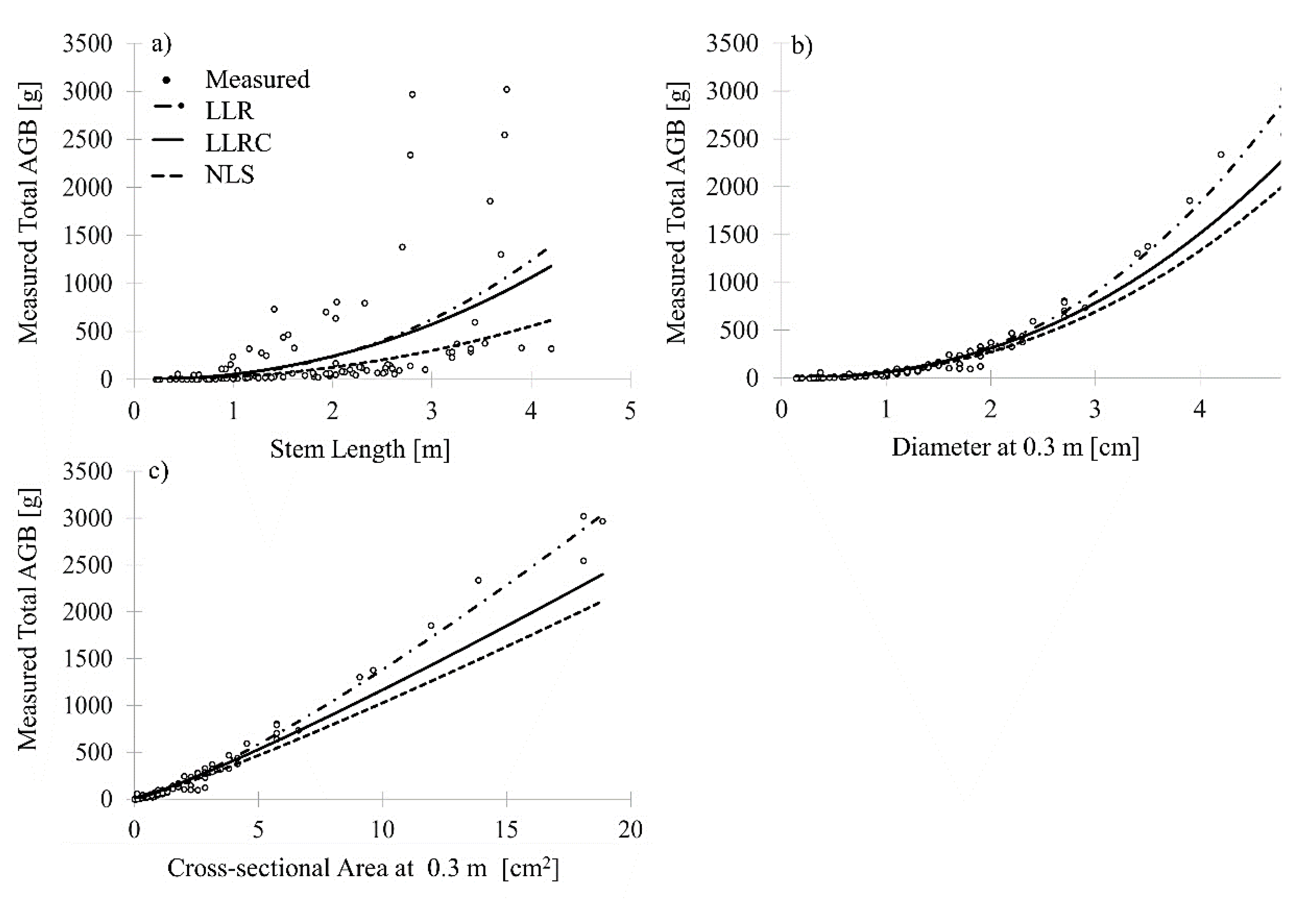
3.3. Comparison of 1D and 2D Variables for Tree Total AGB Prediction

For the short-stature tree AGB equations, diameter measured at 0.3 m stem length resulted in better model fits compared to stem length for each genus and species (Supplementary Material 3, Table S7). For the multispecies data, total AGB prediction using stem length (1D variable) provided the lowest goodness of fit (highest RMSE and lowest R²,

Table 4. Model performance for multispecies tree total AGB prediction using 1D and 2D input parameters (all p values < 0.001).

Model	Dimension	Input Variable	Total Percentage Error (%)	RMSE (g)	R2
LLR	1D	Stem length	−51	529.08	0.285
	1D	Diameter at 0.3 m	−20	188.71	0.987
	2D	Cross-sectional area at 0.3 m	−20	188.41	0.987
LLRC	1D	Stem length	−6	484.83	0.285
	1D	Diameter at 0.3 m	−10	134.00	0.987
	2D	Cross-sectional area at 0.3 m	−9	133.68	0.987
NLS	1D	Stem length	−1	482.77	0.286
	1D	Diameter at 0.3 m	2	62.25	0.988
	2D	Cross-sectional area at 0.3 m	2	62.25	0.988

, Figure 4), while inclusion of stem diameter at 0.3 m, alternatively cross-sectional area at 0.3 m, improved predictions by 87% using LLRC or NLS (Table 4).

For multispecies tree total AGB prediction, the exponent $\alpha$ was greater for the 1D model based on stem length and close to unity for the 1D model diameter at 0.3 m, alternatively 2D model cross-sectional area at 0.3 m (

Table 5. Regression coefficients to predict total AGB for multispecies trees with LLRC and NLS.

	Variable	LLRC β	NLS β	LLRC α	NLS α
Multispecies trees	Stem length	28.962	45.8224	2.132	2.380
	Diameter at 0.3 m	57.111	59.0721	2.272	2.479
	Cross-sectional area at 0.3 m	75.189	79.6818	1.136	1.240

). The 2D cross-sectional area model produced equivalent results compared to the 1D diameter model but allowed to effectively reconcile tree with shrub AGB predictions. The combined prediction of shrub and tree AGB has not been developed for this study region yet, but would allow the prediction of AGB for boreal short-stature shrubs and trees (<4.5 m) as well as tall-stature trees (>4.5 m) in just a few steps (see Section 3.5). When transferring these allometric models to different areas within the region, we recommend measuring the diameter at 0.3 m stem length.

3.4. Comparison of Regression Models for Tree Total AGB Prediction

For the prediction of tree total AGB per genus/species and all genera/species combined, NLS achieved the lowest RMSE, highest R², and lowest total percentage error compared to measured biomass (<−5%–4%), while the dependent and independent variables were significantly related (p < 0.001, Table 4 and Table S7). LLR predictions resulted in the highest RMSE, similar R², and highest total percentage error relative to the measured biomass compared to LLRC and NLS for each genus/species and for all data combined. The single exception was for predicting total AGB for Picea spp. based on stem length (Table S7). Using LLR, the prediction based on stem length resulted in an underestimation of total AGB of −51% and an underestimation of −20% when using diameter or cross-sectional area, respectively, as input variable for the multispecies models. LLRC had comparably lower RMSE, similar R², and underestimated total multispecies AGB by −6% (stem length) to <−10% (diameter at 0.3 m, cross-sectional area at 0.3 m). In order to address potential heteroscedasticity effects, we have provided the regression coefficients for both NLS and LLRC models with cross-sectional area (measured at 0.3 m stem length) as predictor variable (Supplementary Material 2, Table S4).

3.5. Comparison of Regression Models for General Shrub and Tree Total AGB Prediction

The prediction of total AGB for shrubs and trees combined resulted in similar predictive capability to multispecies shrub and multispecies short-stature trees (R² ≥ 0.770, p < 0.001). This was determined using the 2D independent variable of cross-sectional area, measured at the base for shrubs and at 0.3 m stem length for trees (

Table 6. Model performances for combined general shrub and tree total AGB prediction (all p values < 0.001).

Model	Dimension	Input Variable	Total Percentage Error (%)	RMSE (g)	R2
LLR	1D	Stem length	−44.15	378.72	0.249
	2D	Cross-sectional area	−11.17	202.17	0.770
LLRC	1D	Stem length	0.03	381.27	0.249
	2D	Cross-sectional area	0.02	206.37	0.770
NLS	1D	Stem length	22.53	292.51	0.500
	2D	Cross-sectional area	2.28	94.80	0.776

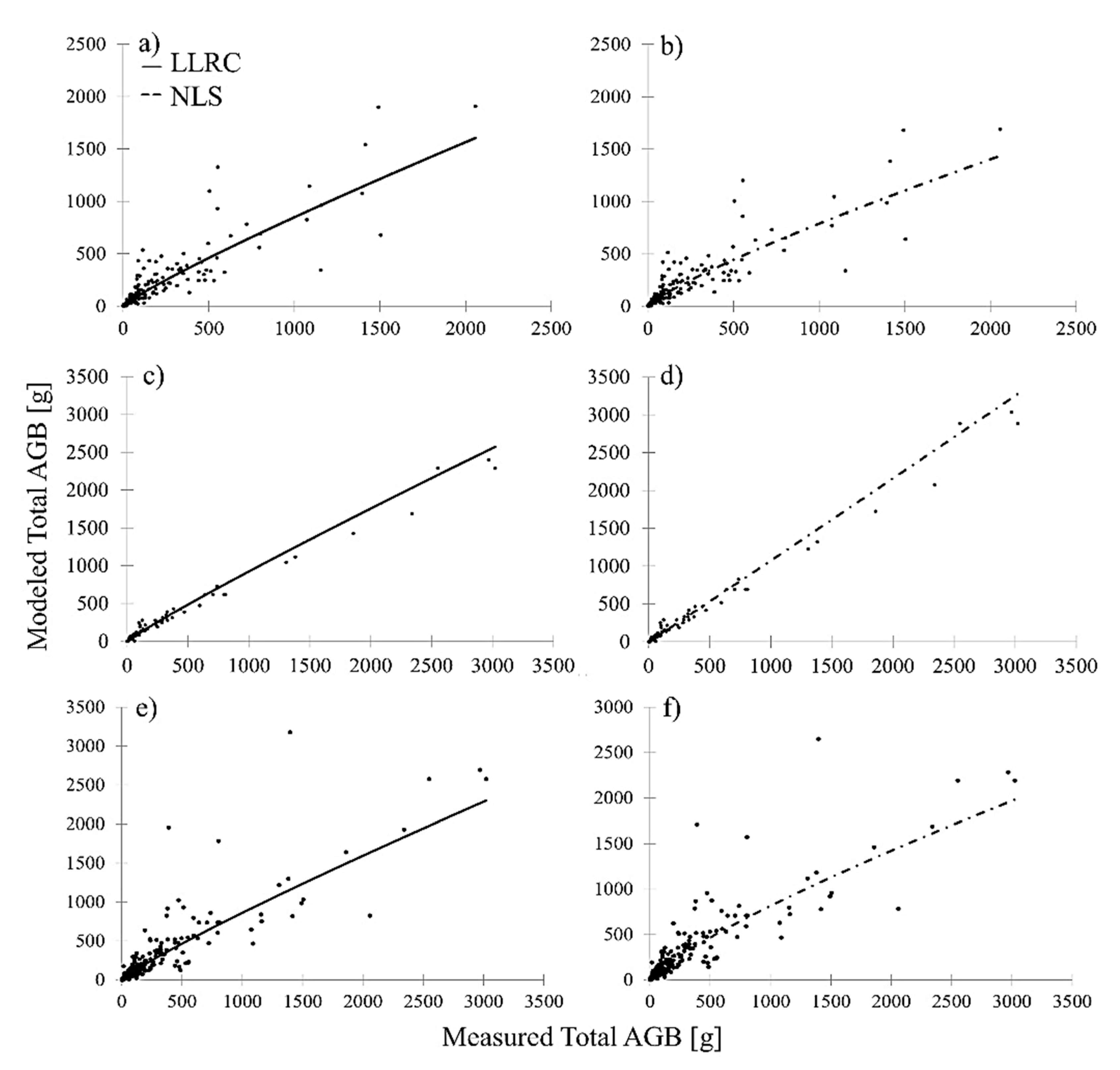
, Figure 5). Relating modeled total AGB to measured total AGB showed no evident bias in the 2D-based prediction of combined shrub and tree AGB in comparison to 3D multispecies shrub and 2D multispecies tree AGB models. This is depicted in Figure 6, which shows modeled AGB in relation to measured AGB of the 2D general shrub and tree AGB model (Figure 6e,f) in comparison to the 3D multispecies shrub (Figure 6a,b) and 2D multispecies tree (Figure 6b,c) AGB models. Similar to the multispecies shrub models, NLS achieved the lowest RMSE and highest R² (RMSE = 94.80 g, R² = 0.776). The RMSE of model LLR increased by 53% (RMSE = 202.17 g, R² = 0.770) and by 54% for the LLRC model (RMSE = 206.37 g, R² = 0.770). Compared to Ali et al. [27], who derived best model fits for combined shrub and tree AGB prediction using diameter of the longest stem and total plant height combined, our model results show that AGB of boreal plants can be predicted with a simpler one-variable model using cross-sectional area. For our AGB models based on cross-sectional area, the exponent $\alpha$ was greater for the 1D model based on stem length and close to unity for the 2D model cross-sectional area at 0.3 m (

Table 7. Regression coefficients to predict total AGB for general shrubs and trees with LLRC and NLS.

	Variable	LLRC β	NLS β	LLRC α	NLS α
General shrubs and trees	Stem length	63.944	142.299	1.816	1.447
	Cross-sectional area	94.917	128.802	1.084	0.979

). However, stem length of shrubs and trees was also weakly related to measured total AGB (p < 0.001, Table 6) and thus represents an alternative to cross-sectional area, which has potential for use in rapid field measurement or non-invasive observation situations (e.g., remote sensing via airborne lidar) where it may be acceptable to trade accuracy at the individual sample-level for greater overall population representation. For model transfer purposes, we recommend the use of LLRC regression coefficients and correction factor in order to address heteroscedasticity.

4. Conclusions

Our analysis has shown that AGB of shrubs can be modeled with higher accuracies when using a 3D field variable, such as volume. Small-stature tree AGB can be most accurately predicted with the stem diameter measured at 0.3 m stem length. In addition, we found that shrub AGB can be reconciled with small-stature tree AGB when using total stem cross-sectional area as the predictor variable. Based on the two best models, we have provided regression coefficients and error statistics for the modeling of short-stature shrub and tree AGB for the region of sporadic to discontinuous permafrost in NWT, Canada. For model uncertainty propagation to total AGB predictions, we have provided the standard error of each model coefficient. We have provided species- and genus-specific as well as multispecies allometric models for shrubs and trees commonly found in boreal forest and peatland ecosystems. These equations are necessary for improving understanding and quantification of biomass change and the potential implications for carbon pools in northern environments, which are highly susceptible to climate change.

References

1. Flannigan, M.D.; Logan, K.A.; Amiro, B.D.; Skinner, W.R.; Stocks, B.J. Future area burned in Canada. Clim. Chang. 2005, 72, 1–16. [Google Scholar] [CrossRef]
2. Gauthier, S.; Bernier, P.; Burton, P.J.; Edwards, J.; Isaac, K.; Isabel, N.; Jayen, K.; Le Goff, H.; Nelson, E.A. Climate change vulnerability and adaptation in the managed Canadian boreal forest. Environ. Rev. 2014, 22, 256–285. [Google Scholar] [CrossRef]
3. IPCC. Contribution of Working Groups I, II and III to the Fifth Assessment Report of the Intergovernmental Panel on Climate Change. In Climate Change 2014. Synthesis Report; Core Writing Team, Pachauriand, R.K., Meyer, L.A., Eds.; IPCC: Geneva, Switzerland, 2014; p. 151. [Google Scholar]
4. Berner, L.T.; Beck, P.S.A.; Bunn, A.G.; Lloyd, A.H.; Goetz, S.J. High-latitude tree growth and satellite vegetation indices: Correlations and trends in Russia and Canada (1982–2008). J. Geophys. Res. 2011, 116, G01015. [Google Scholar] [CrossRef] [Green Version]
5. Myers-Smith, I.H.; Forbes, B.C.; Wilmking, M.; Hallinger, M.; Lantz, T.C.; Blok, D.; Tape, K.D.; Macias-Fauria, M.; Sass-Klaassen, U.; Lévesque, E.; et al. Shrub expansion in tundra ecosystems: Dynamics, impacts and research priorities. Environ. Res. Lett. 2011, 6, 045509. [Google Scholar] [CrossRef] [Green Version]
6. Goetz, S.J.; MacK, M.C.; Gurney, K.R.; Randerson, J.T.; Houghton, R.A. Ecosystem responses to recent climate change and fire disturbance at northern high latitudes: Observations and model results contrasting northern Eurasia and North America. Environ. Res. Lett. 2007, 2, 045031. [Google Scholar] [CrossRef]
7. Goulden, M.L.; Mcmillan, A.M.S.; Winston, G.C.; Rocha, A.V.; Manies, K.L.; Harden, J.W.; Bond-Lamberty, B.P. Patterns of NPP, GPP, respiration, and NEP during boreal forest succession. Glob. Chang. Biol. 2011, 17, 855–871. [Google Scholar] [CrossRef] [Green Version]
8. Chasmer, L.; Hopkinson, C. Threshold loss of discontinuous permafrost and landscape evolution. Glob. Chang. Biol. 2017, 23, 2672–2686. [Google Scholar] [CrossRef] [PubMed]
9. Helbig, M.; Chasmer, L.E.; Kljun, N.C.; Quinton, W.L.; Treat, C.C.; Sonnentag, O. The positive net radiative greenhouse gas forcing of increasing methane emissions from a thawing boreal forest-wetland landscape. Glob. Chang. Biol. 2017, 23, 2413–2427. [Google Scholar] [CrossRef] [Green Version]
10. Kurz, W.; Shaw, C.; Boisvenue, C.; Stinson, G.; Metsaranta, J.; Leckie, D.; Dyk, A.; Smyth, C.; Neilson, E. Carbon in Canada’s boreal forest—A synthesis. Environ. Rev. 2013, 21, 260–292. [Google Scholar] [CrossRef]
11. Berner, L.T.; Alexander, H.D.; Loranty, M.M.; Ganzlin, P.; Mack, M.C.; Davydov, S.P.; Goetz, S.J. Biomass allometry for alder, dwarf birch, and willow in boreal forest and tundra ecosystems of far northeastern Siberia and north-central Alaska. For. Ecol. Manag. 2015, 337, 110–118. [Google Scholar] [CrossRef]
12. Berner, L.T.; Jantz, P.; Tape, K.D.; Goetz, S.J. Tundra plant above-ground biomass and shrub dominance mapped across the North Slope of Alaska. Environ. Res. Lett. 2018, 13, 035002. [Google Scholar] [CrossRef] [Green Version]
13. Myers-Smith, I.H.; Kerby, J.T.; Phoenix, G.K.; Bjerke, J.W.; Epstein, H.E.; Assmann, J.J.; John, C.; Andreu-Hayles, L.; Angers-Blondin, S.; Beck, P.S.; et al. Complexity revealed in the greening of the Arctic. Nat. Clim. Chang. 2020, 10, 106–117. [Google Scholar] [CrossRef] [Green Version]
14. Lambert, M.-C.; Ung, C.-H.; Raulier, F. Canadian national tree aboveground biomass equations. Can. J. For. Res. 2005, 35, 1996–2018. [Google Scholar] [CrossRef]
15. Ung, C.H.; Bernier, P.; Guo, X.J. Canadian national biomass equations: New parameter estimates that include British Columbia data. Can. J. For. Res. 2008, 38, 1123–1132. [Google Scholar] [CrossRef]
16. He, A.; McDermid, G.J.; Rahman, M.M.; Strack, M.; Saraswati, S.; Xu, B. Developing allometric equations for estimating shrub biomass in a boreal fen. Forests 2018, 9, 569. [Google Scholar] [CrossRef] [Green Version]
17. Smith, B.W.; Brand, G.J. Allometric Biomass Equations for 98 Species of Herbs, Shrubs, and Small Trees; Research Note; USDA Forest Service: Washington, DC, USA, 1983; Volume 299, 8p. [Google Scholar]
18. Chojnacky, D.C.; Milton, M. Measuring carbon in shrubs. In Field Measurements for Forest Carbon Monitoring: A Landscape-Scale Approach; Hoover, C.M., Ed.; Springer Science: New York, NY, USA, 2008; pp. 45–72. [Google Scholar]
19. Ecosystem Classification Group. Ecological Regions of the Northwest Territories—Taiga Plains. Department of Environment and Natural Resources; Government of the Northwest Territories: Yellowknife, NT, Canada, 2007. [Google Scholar]
20. Ecosystem Classification Group. Ecological Regions of the Northwest Territories—Taiga Shield. Department of Environment and Natural Resources; Government of the Northwest Territories: Yellowknife, NT, Canada, 2008. [Google Scholar]
21. Ecological Stratification Working Group. A National Ecological Framework for Canada; Agriculture and Agri Food Canada: Ottawa/Hull, ON, Canada, 1995. [Google Scholar]
22. Flanagan, L.B.; Syed, K.H. Stimulation of both photosynthesis and respiration in response to warmer and drier conditions in a boreal peatland ecosystem. Glob. Chang. Biol. 2011, 17, 2271–2287. [Google Scholar] [CrossRef]
23. Baskerville, G.L. Use of logarithmic regression in the examination of plant biomass. Can. J. For. 1972, 2, 49–53. [Google Scholar]
24. Bond-Lamberty, B.; Wang, C.; Gower, S.T. Aboveground and belowground biomass and sapwood area allometric equations for six boreal tree species of northern Manitoba. Can. J. For. Res. 2002, 32, 1441–1450. [Google Scholar] [CrossRef]
25. Mascaro, J.; Labs, P.; Litton, C.M.; Schnitzer, S. Minimizing Bias in Biomass Allometry: Model Selection and Log-Transformation of Data. Biotropica 2011, 43, 649–653. [Google Scholar] [CrossRef] [Green Version]
26. R Core Team. R: A Language and Environment for Statistical Computing; R Foundation for Statistical Computing: Vienna, Austria, 2020. [Google Scholar]
27. Ali, A.; Xu, M.S.; Zhao, Y.T.; Zhang, Q.Q.; Zhou, L.L.; Yang, X.D.; Yan, E.R. Allometric biomass equations for shrub and small tree species in subtropical China. Silva. Fenn. 2015, 49, 1–10. [Google Scholar] [CrossRef] [Green Version]
Figure 1. (a) Field locations of destructive sampling of shrub and short-stature tree AGB in peatlands and upland forest ecosystems. Field locations are distributed across the (b) mid-boreal Taiga Plains and high-boreal Taiga Shield ecoregions of the Northwest Territories, Canada.
Forests 11 01207 g001
Figure 2. (a) Example of a transect traversing a burned upland forest into peatland (fire year 2015); (b,c) illustration of a Betula glandulosa shrub individual growing along the transect before and after destructive sampling, respectively.
Forests 11 01207 g002
Figure 3. LLRC, LLR, and NLS model fits for each 1D (a,b), 2D (c), and 3D (d) predictor variable utilized to model total AGB for multispecies shrubs.
Forests 11 01207 g003
Figure 4. LLRC, LLR, and NLS model fits for each 1D (a,b), and 2D (c) predictor variable utilized to model total AGB for multispecies trees.
Forests 11 01207 g004
Figure 5. LLRC, LLR, and NLS model fits for the 2D predictor variable utilized to model total AGB for general shrubs and trees: (a) stem length and (b) cross-sectional area.
Forests 11 01207 g005
Figure 6. Measured total AGB related to modeled total AGB using LLRC and NLS for the 3D-based equations for multispecies shrubs (a,b) and the 2D-based equations for multispecies trees (c,d) as well as general shrubs and trees (e,f).
Forests 11 01207 g006