Article

Baseline of Carbon Stocks in Pinus radiata and Eucalyptus spp. Plantations of Chile

by
Guillermo F. Olmedo
1,*,
Mario Guevara
2,
Horacio Gilabert
3,4,
Cristián R. Montes
5,
Eduardo C. Arellano
3,4,6,
Beatriz Barría-Knopf
1,
Francisco Gárate
1,
Pablo Mena-Quijada
1,
Eduardo Acuña
7,
Horacio E. Bown
8 and
Michael G. Ryan
9,10
1
Investigaciones Forestales Bioforest S.A., Camino a Coronel, Km. 15, Concepción 4030000, Chile
2
Department of Plant and Soil Sciences, University of Delaware, Newark, DE 19716, USA
3
Centro Interdisciplinario de Cambio Global, Pontificia Universidad Católica de Chile, Av. Vicuña Mackenna 4860, Santiago 7820436, Chile
4
Departamento de Ecosistemas y Medio Ambiente, Pontifica Universidad Católica de Chile, Av. Vicuña Mackenna 4860, Santiago 7820436, Chile
5
Warnell School of Forestry and Natural Resources, The University of Georgia, Athens, GA 30602, USA
6
Center of Applied Ecology and Sustainability (Capes), Pontificia Universidad Católica de Chile, Santiago 9160000, Chile
7
Facultad de Ciencias Forestales, Universidad de Concepción, Victorial 631, Concepción 4030000, Chile
8
Facultad de Ciencias Forestales y de la Conservación de la Naturaleza, Universidad de Chile, Casilla 9206, Santiago 9160000, Chile
9
USDA Forest Service, Rocky Mountain Research Station, Fort Collins, CO 80526, USA
10
Department of Ecosystem Science & Sustainability and Natural Resource Ecology Laboratory, Colorado State University, Fort Collins, CO 80523-1499, USA
*
Author to whom correspondence should be addressed.
Forests 2020, 11(10), 1063; https://doi.org/10.3390/f11101063
Submission received: 2 September 2020 / Revised: 24 September 2020 / Accepted: 29 September 2020 / Published: 30 September 2020
(This article belongs to the Special Issue Forest Silviculture and Carbon Sequestration in a Changing Climate)

Abstract

:
Forest plantations have a large potential for carbon sequestration, playing an important role in the global carbon cycle. However, despite the large amount of research carried out worldwide, the absolute contribution of forest plantations is still incomplete for some parts of the world. To help bridge this gap, we calculated the amount of C stock in three fast growing forest species in Chile. Carbon pools in above-ground and below-ground biomass, forest floor, and soil were considered for this analysis. Across the plantation forests of Chile, carbon accumulated in the above-ground biomass was 181–212 Mg · ha 1 for Pinus radiata, 147–180 Mg · ha 1 for Eucalyptus nitens, and 95–117 Mg · ha 1 for Eucalyptus globulus (age 20–24 years for P. radiata and 10–14 years for Eucalyptus). Total C stocks were for 343 Mg · ha 1 for P. radiata, 352 Mg · ha 1 for E. nitens, and 254 Mg · ha 1 for E. globulus, also at the end of a typical rotation. The carbon pool in the forest floor was found to be significantly lower (less than 4% of the total) when compared to the other pools and showed large spatial variability. Our results agree with other studies showing that 30–50% of the total C stock is stored in the soil. The baseline data will be valuable for modelling C storage changes under different management regimes (changes in species, rotation length and stocking) and for different future climates. Given the contribution of soils to total carbon stocks, special attention should be paid to forest management activities that affect the soil organic carbon pool.

1. Introduction

Global climate is changing: air and subsurface ocean temperatures are rising due to greenhouse gases accumulating at the Earth’s atmosphere [1,2]. These global temperature increases cannot be explained by natural variations alone without considering the observed increase in anthropogenic greenhouse gas concentrations [3]. There is unequivocal evidence that the concentrations of carbon dioxide (CO 2 ), methane, and nitrous oxide have increased over the last few centuries [2,4]. Because CO 2 is the primary anthropogenic greenhouse gas emitted, two strategies can lower the amount of CO2 in the atmosphere: reducing and avoiding emissions, and increasing carbon sequestration and land carbon uptake [5]. Afforestation and reforestation in managed forests worldwide play a key role in regulating the global C cycle and are relevant options for climate change mitigation [6]. In both cases, carbon pools and carbon sequestration are increased, especially in degraded or non-forested areas. Such practices could have a large potential impact on CO 2 sequestration and co-benefits such as increased ecosystem services and biodiversity and improved soil quality [7,8]. Because climate is changing, understanding the role of managed forests across different site conditions, in controlling the fate of land carbon uptake for future climate will be critical for C projections [9,10,11]. Baseline information for C stocks on managed forests is a valuable knowledge tool contributing towards monitoring C stock changes and to identify the effectiveness of forest management strategies, afforestation, and reforestation practices on C storage [12,13,14]. One challenge to generate accurate baselines for forest C stocks is to increase the availability of ground-based forest data and information [15,16]. Increased availability of C datasets would be needed to monitor the current and past efficiency of forest management activities in maintaining primary productivity and high carbon uptake rates. Another challenge is to build institutional alliances to increase the availability of C datasets of managed forest to provide robust C cycle reports with a national perspective.
Carbon pools can be partitioned into four C stock components: (a) above-ground biomass (wood and leaves), (b) below-ground biomass (roots), (c) soil C in mineral soil, and (d) soil organic layer (forest floor, shed vegetative parts existing in various stages of decomposition above the soil surface) [17]. The role of forest plantations in the regional to global C cycle has gaps in spatial and temporal variability, because there are large geographical areas where accurate forest C estimates are not available. Currently, knowledge of C stocks in plantations could be improved by using empirical data generated by forest inventory [17,18] and other management measurements in commercial forests across countries where natural and plantation forests are managed.
In Chile, the industrial forest sector relies on three introduced fast-growing species: Pinus radiata D. Don (PIRA), Eucalyptus globulus Labill (EUGL) and, Eucalyptus nitens (Deane and Maiden) Maiden (EUNI) plantations [19]. In these plantations, standing yields and above-ground biomass stocks are monitored using repeated sampling, a procedure called forest inventory. These inventories capture tree and plot-level information representing a point in time. Attributes commonly evaluated are stand density, mean top height, basal area, total and commercial volume, and log assortments. Forest inventories are done at different stages of stand development: after establishment, before or after thinning or pruning, and before harvest. Although plantation forests are periodically surveyed, forest inventories only yield estimates of above-ground biomass; C stocks in soil, forest floor and below-ground live biomass are generally not measured and estimated with biomass expansion factors (BEFs). Because soil C is often the largest C pool in forests [20], a group of scientists from 39 public and private institutions systematized and made available the Chilean Soil Organic Carbon database [21] to better describe the soil organic carbon pool of forest plantations.
Across the entire world, C cycle-related estimates and datasets have been used to develop hypothesis about forest management practices and the effectiveness of afforestation to mitigate the negative effects of climate change [7,22,23,24,25,26,27,28]. Bastin et al. [29] described the potential impact of reforestation at the global scale to mitigate climate change. Nevertheless, the key hypotheses presented by Bastin et al. [29], that the restoration of trees remains among the most effective strategies for climate change mitigation, have been criticized due to the oversimplification in the role of plant and atmosphere interactions and due to the need for accurate estimates of C stocks on each pool, especially when considering soils, climate and land-use changes [30,31,32,33]. In Chile, a recent study highlighted the impacts of afforestation subsidies in forest cover, carbon sequestration, and biodiversity [34]. As the main conclusions were drawn from the above-ground C densities of the different land-use classes, having a consistent data set is crucial to support their findings. In this sense, the quality of C cycle related datasets for these and future studies is critical to quantify the real feedback between C stocks, land-use changes, and climate change mitigation [35].
Considering the uncertainties in the role of forest plantations on carbon sequestration in Chile the objective of this study was to generate a comprehensive data set of C stocks for managed forests of Chile integrating public and private data. Thereby, we ask the following research questions: (1) How are C stocks distributed among the four C pools? (2) How does C in above-ground biomass vary with species and forest age? (3) What is the capacity of forest plantations to store C across the different forest regions of Chile? and (4) How does the capacity of forests to store C vary with climate and soil type? We aim to answer these questions using a data-driven approach, to establish a 2019 baseline for the C stored in managed forests of Chile by component, and to understand how C storage varies across regions, climate, and soil types.

2. Materials and Methods
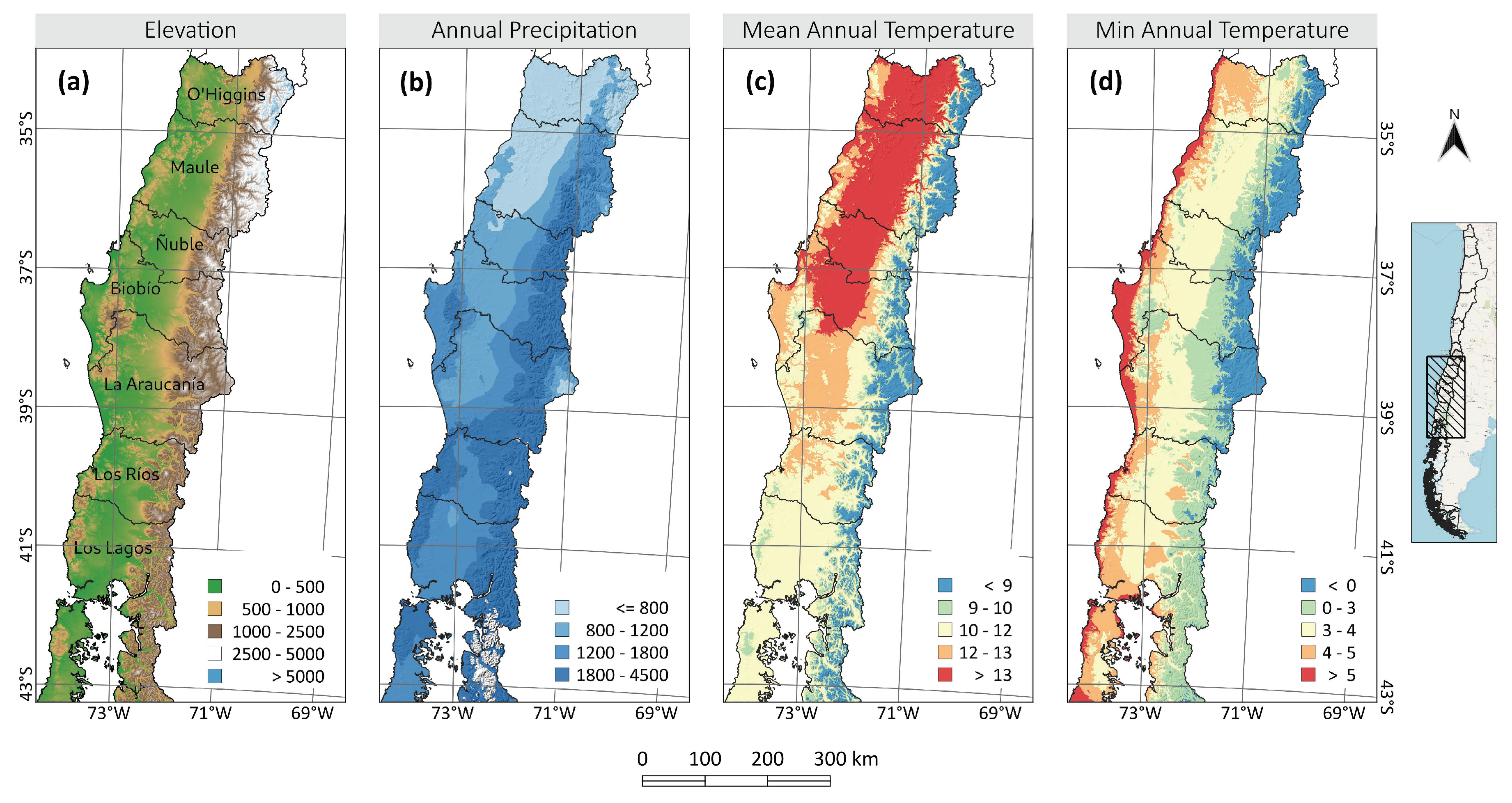
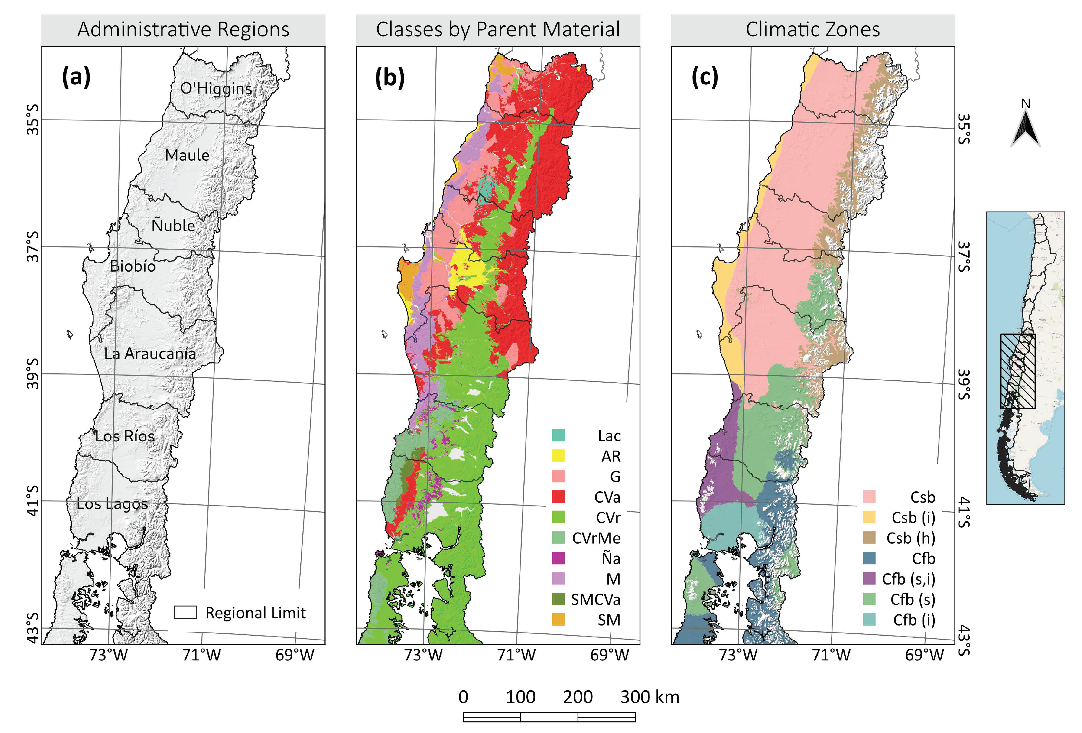
In this section we describe the environmental and soil conditions where forest plantations of PIRA, EUGL and EUNI grow in Chile (Section 2.1) and describe how public and private data are combined to estimate C stocks for the four components (Figure 1). The contribution of above-ground biomass and roots (Section 2.2) to C stocks was estimated using forest simulation models calibrated with forest inventory data. To estimate 0–30 cm mineral soil (Section 2.3) and soil organic layer (forest floor) C stocks (Section 2.4) a digital soil mapping strategy was used to extrapolate sample data.
Based on the compiled data and simulations, we build maps of soil, litter, above- and below-ground C stock for the year 2019, showing the spatial distribution of C stocks across regions, climates, and soils (Section 2.5 and Section 2.6).

2.1. Area of Study

The study area was 493,112 ha of PIRA plantations, 108,640 ha of EUGL and 58,766 ha of EUNI located in central Chile, from the Maule (latitude 35° 14 ) to the Los Ríos (latitude 40° 6 ) administrative regions. This area has large variability in climate, topography and soils (Figure 2).
The northernmost part of this research is situated in the O’Higgins region, where forest plantations are mainly located on granitic soils in the Coastal Andes range. The climate in this area is Mediterranean with a coastal influence. In the Maule region, forest plantations are mostly found in the coastal mountain range and the central plains on soils of metamorphic and granitic origin [36]. The climate is warm temperate, with a sea coast influence during summer. Precipitation occurs mainly in 4 months during the winter season. Forest plantations in the Ñuble region are located mainly in the coastal ranges and in the Andes foothills, over granitic-metamorphic and volcanic ash soils, respectively. These sectors are highly productive, with a warm temperate climate. This region has four to five dry months. In the Biobío region, the forest plantations are mainly in the coastal plains of the Gulf of Arauco on soils of marine sediments and in the coastal range on soils of metamorphic origin. The climate is temperate-rainy, with dry periods during summer and with rain for the rest of the year. A few plantations in this region are located in the central plains, on volcanic sandy soils, not very productive, and where rainfall does not exceed 700 mm per year. From the Araucanía to Los Lagos region, forest plantations are mainly found between the coastal range and the central plains. These plantations are on highly productive volcanic ash soils deposits with a temperate rainy climate.
Management schemes for PIRA can be grouped in 3 classes: (i) Pulp schema with no pruning or thinning; (ii) multipurpose schema including thinning but no pruning and, (iii) intensive schema: with pruning and thinning and different final tree densities. According to Buchner et al. [37], in 2018, 23% of the PIRA area was managed under schema i, 27% under schema ii, and 50% under schema iii. EUGL and EUNI are generally managed without pruning or thinning.

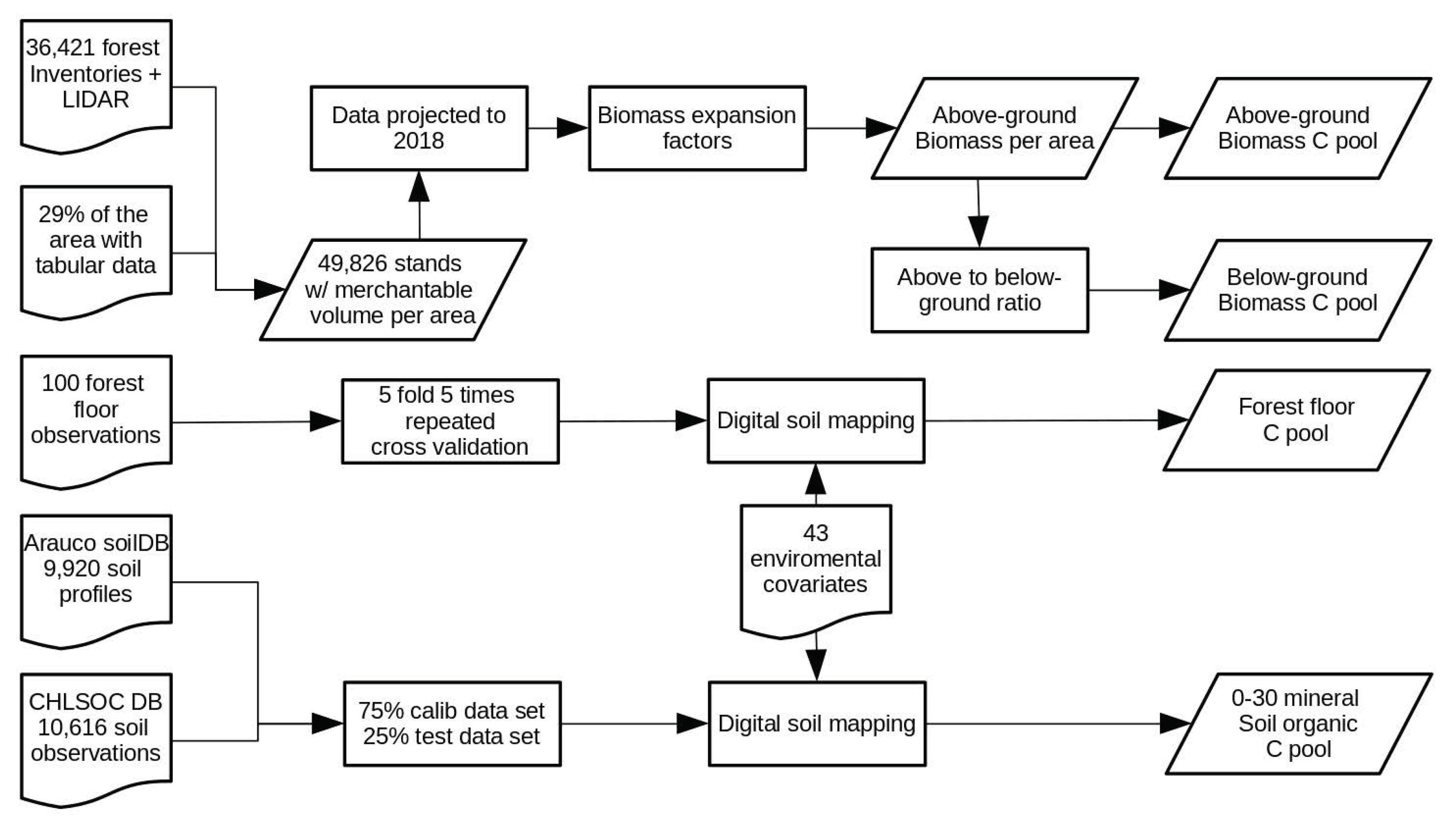
2.2. Above-Ground and Below-Ground Biomass Carbon Pool

Biomass estimates were collected for 49,826 different stands of three species: PIRA (n = 40,363), EUGL (n = 6952) and EUNI (n = 2511) adding up to 659,140 hectares of forest plantations and representing 30% of the forests plantations in the study area. Merchantable volume of growing stock was measured using three methods: direct field measurements, LIDAR measurements and predictions from yield tables. On 63% of the stands, direct field measurements, involving 36,421 survey sites, were taken. These field measurements were then projected to year 2018 using a locally developed forest growth model, ’Modelo Nacional de Simulación’ (MNS) [38]. On 30% of the area of EUGL and EUNI, representing the 7% of the total area, measurements were carried out using LIDAR data (Point density 6 points m 2 ) and a model linking LIDAR-derived-metrics to ground-truth data [39]. On the remaining 29% of the stands, merchantable volume of growing stock was calculated using a yield table, relating yield to the combination of specie, age, number of trees per unit of area, and management schema. For the three methods, the total volume per stand was determined as the sum of the volumes of individual trees within its given area. The volume of each tree was calculated using a taper function integrated between two portions of the stem (tree base and tree top) [40,41]. The equations used were generated by MNS and were adjusted for each species and productivity zone.
Merchantable volume of growing stock was then converted directly to total biomass using biomass conversion and expansion factors (BCEF) following the procedure suggested in [17] (Table 1). Values used were the corresponding for the ’Temperate’ climatic zone, forest type ’hardwoods’ for EUGL and EUNI, and ’pines’ for PIRA. The factors with the growing stock level (m 3 ) (i.e., current biomass) as BCEFs tend to decrease as growing stock density increases, because the ratio of merchantable volume to total volume increases with growing stock level. Carbon stock in above-ground biomass was then estimated by multiplying biomass by the carbon fraction of dry matter (DM). This procedure is summarized using the following equation:
CAGB = Vol · BCEF s · CF
where CAGB is the carbon content of the above-ground biomass [Mg C · ha 1 ]; Vol is the merchantable volume of the growing stock per area [m 3 · ha 1 ]; BCEFs is biomass conversion and expansion factors for expansion of merchantable growing stock level to above-ground biomass [Mg dry matter (DM) · m 3 ]; CF is the carbon fraction of dry matter [Mg DM · m 3 ]. For CF we used 0.48 for PIRA and 0.51 for EUGL and EUNI, as suggested in [17].
Below-ground biomass was estimated as a ratio of above-ground biomass following the approach suggested by [17] (Table 2). Ratio used was selected according to the species planted and its above-ground biomass category for the Domain ’Temperate’. Conversion from biomass volume to carbon content was done using the same approach as in above-ground biomass using the following equation:
CBGB = Vol · R · BCEF s · CF
where CBGB is the carbon density of the below-ground biomass [Mg · ha 1 ]; Vol is the merchantable volume of growing stock per area [m 3 · ha 1 ]; R is ratio of below-ground biomass to above-ground biomass [Mg DM below-ground biomass · (Mg DM above-ground biomass) 1 ]; BCEF s is biomass conversion and expansion factors for expansion of merchantable growing stock level to above-ground biomass [Mg DM · m 3 ]; CF is the carbon fraction of the dry matter [Mg C · (Mg DM) 1 ].

2.3. Soil Organic Carbon Pool

The soil organic carbon pool across the plantation areas was assessed using measured samples extrapolated by Digital Soil Mapping (DSM) [42], a reference framework to quantify the spatial variability soil attributes and their response to environmental variation. Soil carbon values are modeled as a function of environmental covariates that are surrogates of soil weathering conditions (Table A1). We used 20,536 observations (soil profiles and top soil auger samples) for the 0–30 cm of mineral soil depth by merging two datasets. The first database comprises a collection of 9920 soil profiles measured on forest plantations just after harvest between 1997 and 2018. Profiles were sampled following the guidelines for describing and sampling soils presented at [43] on representative sites of stand just after harvest. The second database comprises 10,616 soil observations (including soil profiles and top soil samples) spatially selected from the Chilean Soil Organic Carbon database (CHLSOC) [21]. The CHLSOC includes soil carbon values on different land uses (e.g., native forests, agriculture, grasslands). Combined, both datasets allowed us to better model the soil-landscape relationship across the different regions of Chile.
The combined soil carbon dataset was randomly divided into two datasets of 75 and 25% that were used for training (i.e., model building) and testing (i.e., model validation) of predicted soil carbon values. The prediction models were based on the Random Forest algorithm, a popular ensemble of regression trees based on bagging predictors [44]. This algorithm has proven to be efficient for mapping soil carbon across Chile and Latin America [45,46,47,48]. This algorithm was used to model soil organic carbon based on the statistical relationships between soil carbon and environmental covariates representing soil forming factors. The environmental covariates used as prediction factors for soil carbon values were prepared using a spatial support of 90 × 90 m grids and derived from remote sensing, terrain analysis, climate gridded datasets or thematic maps (Table A1). The Random Forest algorithm was implemented following the guidelines proposed in previous work [49,50] and evaluated using the testing dataset. The uncertainty of model predictions are also calculated using a quantile based form of Random Forests [51], which estimates a pixel-wise measure of uncertainty. The main assumption of this approach is that the mean of the predictions is similar or not different to the mean of the estimated model based uncertainty. From this methodology we obtain a regional soil C estimate (with an associated uncertainty map) that we further generalize to the forest stand level for C reporting purposes.

2.4. Forest Floor Carbon Pool

Forest floor C plays a major role regulating soil and atmosphere feedbacks [52], but there are no datasets for soil organic layer (forest floor) C for Chile. For this study, forest floor was sampled using a conditioned Latin hypercube sampling design [53]. The sampling design considered the planted tree species, the age of the plantation and the soil organic carbon stock to define the sampling universe. This sampling design methods selects a sample in order that the multivariate distribution of the sampling variables is maximally stratified. A total of 100 sites were sampled with 5 replicates per site with a 25 cm circular sampling frame. The five samples per site were pooled by site. Humus and litter thickness, and bulk density were measured on site, and organic carbon content was analyzed in a laboratory by using a LECO analyzer (LECO Corporation, St. Joseph, MI, USA).
The estimated forest floor C stocks were combined with environmental variables (Table A1) to implement the same modeling strategy used for mapping soil C values and their uncertainties (Random Forest for prediction and quantile Random Forest for calculating uncertainty). Different models were estimated to predict the soil organic carbon content, layer thickness and bulk density for the humus and the litter layers. To evaluate model fit, a repeated cross validation with 5 groups (folds) and 5 repetitions was applied. The Litter and humus layer organic carbon stock was modeled over a raster grid of 90 × 90 m and then generalized as the mean on a stand basis for reporting.

2.5. Integration of the Results

Above- and below-ground biomass C was estimated on a stand basis based on forest inventories and/or tabulated data. Soil and forest floor information were produced using a DSM approach over a 90 × 90 m grid. The mean value per stand for the soil and forest grid layer was estimated to derive a database including the mean value of the four pools and their total for all 49,835 stands. and each stand was categorized by specie, age, administrative region, soil class and climatic zone.
We present the information aggregated by species, administrative region, climate, and soil parent material (Figure 3). Comparisons by climate were generated by combining the gridded stand C data with the Chile map of Köppen climate classification [54]. For the forest region evaluated, this map presents 2 climate classes using a third-order Köppen–Geiger classifications (Oceanic climates and Mediterranean warm/cool summer climates). The two classes were further divided following Sarricolea et al. [54] using a new criteria to enable the identification of climatic subtleties in 7 sub classes. Mediterranean warm/cool summer climates were divided in 3 classes: Mediterranean warm/cool summer climate (Csb), Mediterranean warm/cool summer climate with a more pronounced coastal influence (Csb(i)) and Mediterranean warm/cool summer climate from highlands (Csb(h)). Ocean climates were divided in 4 categories: Ocean climate (Cfb), Ocean climate with a more pronounced coastal influence and dry summer (Cfb(s,i)), Ocean climate with a dry summer (Cfb(s)) and Ocean climate with a more pronounced oceanic influence (Cfb(i)). Comparisons by soil parent material were generated by combining the gridded stand C data with a soil parent material map obtained from the soil series maps [55,56,57,58,59,60,61,62,63,64] together with the geological map of Chile [65]. This map presents 10 soil classes for the forest region: soils formed over lacustrine parent material (Lac), soils formed from sandy alluvial deposits (AR); soils formed from granitic materials (G); soils formed from old volcanic ashes deposits (CVa); soils formed from recent volcanic ashes deposits (CVr); soils formed from recent volcanic ashes deposits over metamorphic materials (CVrMe); shallow volcanic soils with drainage problems, regionally known as Ñadis [66] (Ña); soils formed over metamorphic parent material (M); soils formed over marine sediments covered by old volcanic ashes (SMCVa) and, soils formed over marine sediments (SM).

2.6. Statistical Comparison of Mean Values

Carbon pools were compared either by geographic region, climatic zones or by soil parent material. To overcome inherent differences between groups, both in distribution form and in variance size, a bootstrap regression was adopted to provide both robustness in the group comparisons, as well as to give insight about the statistical power of each comparison. To do so, the data was split into groups corresponding to l regions, or m climatic zones or n parent materials. The bootstrap algorithm sampled 100 observations with replacement per group and regressed the C pool value with the categorical grouping using a linear model. This process constitutes one realization of the data for further analysis. Comparisons among groups were undertaken using Tukey’s test for each realization. A total of 1000 realizations for this procedure were performed and the number of times a group was found different from the remaining groups was recorded as a success. A comparison thresholds was used to indicate significant differences: 0.05. These comparisons lead to the construction of mean confidence intervals, by using the variance of the values, that allowed for a summary of final comparisons.

3. Results

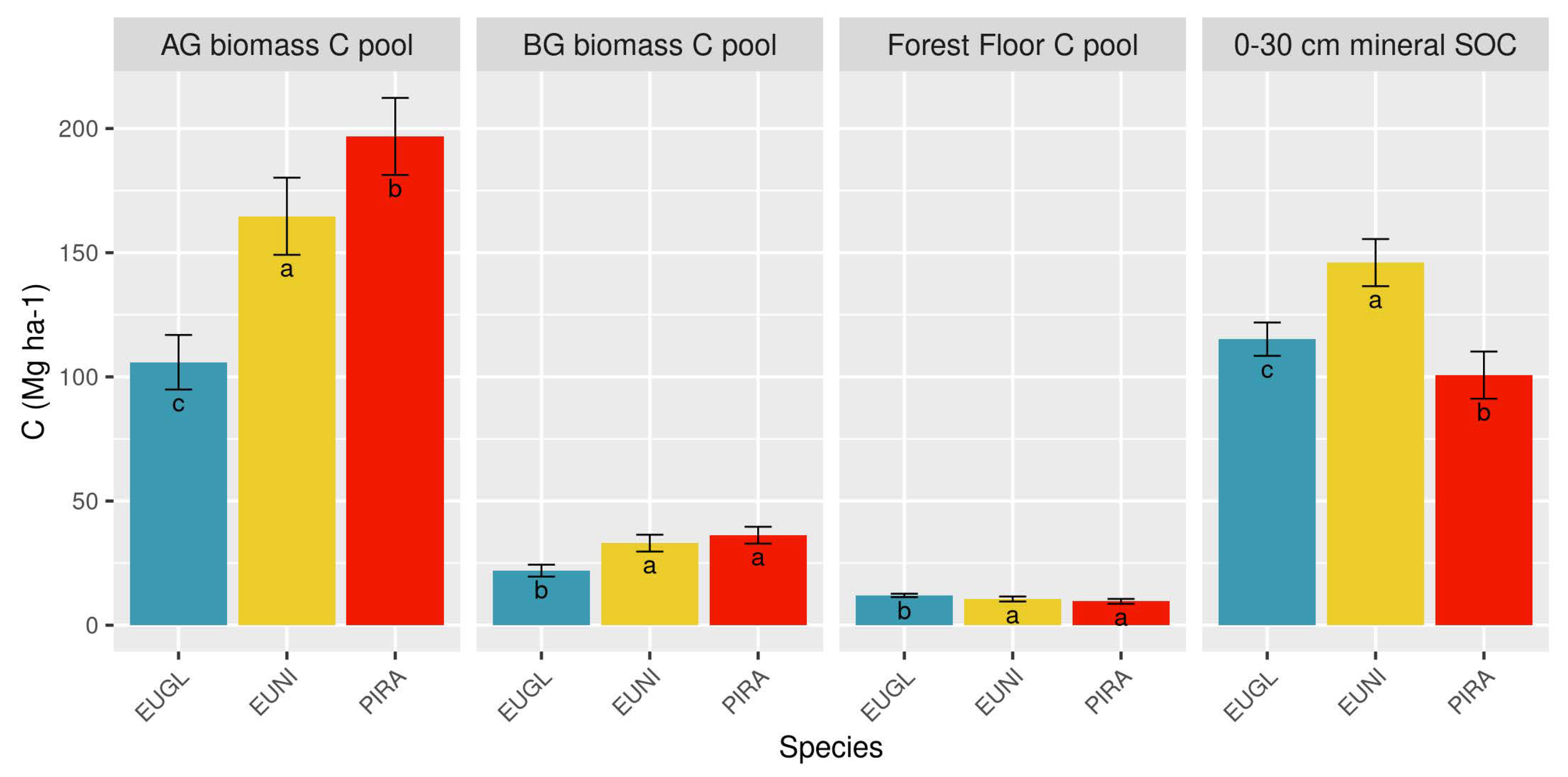
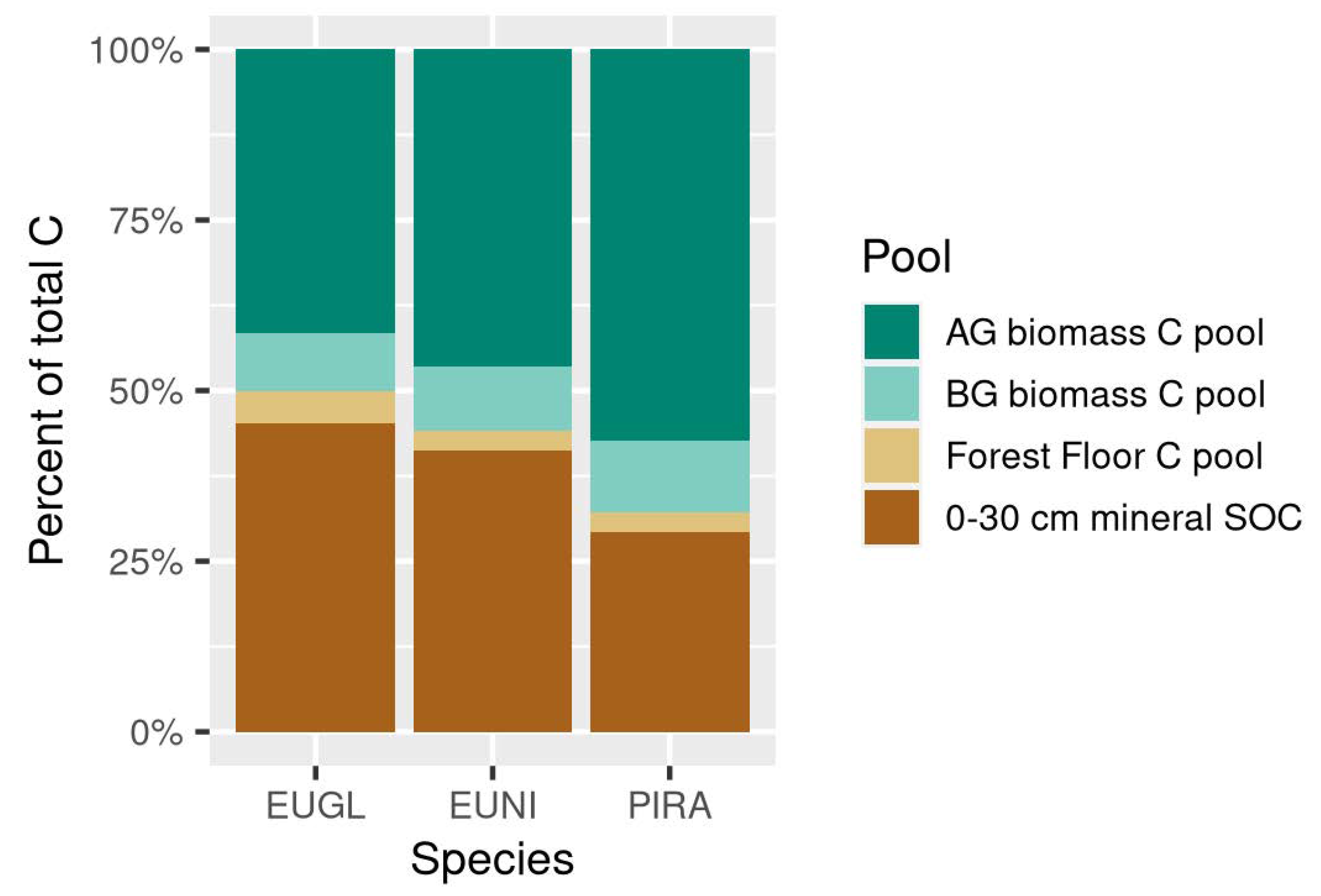
3.1. How Is the C Stock Distributed between the Different C Pools on a Forest Plantation?

At rotation age (20–24 years for PIRA, 10–14 for EUGL and EUNI), average above-ground biomass C was higher in the stands planted with PIRA (196.8 Mg · ha 1 ) followed by EUNI (164.7 Mg · ha 1 ) and then, EUGL (105.9 Mg · ha 1 ). Below-ground biomass C pool did not differ between PIRA and EUNI, (36.2 and 33.0 Mg · ha 1 ) but was lower for EUGL (22.0 Mg · ha 1 ). Organic layer soil C (forest floor C) was considerably lower than the other pools, similar for EUNI and PIRA (10.5 and 9.6 Mg · ha 1 ) and slightly higher for EUGL (12.0 Mg · ha 1 ). 0–30 cm mineral soil carbon was higher for EUNI (146.0 Mg · ha 1 ) lower values for EUGL (115.2 Mg · ha 1 ) and PIRA (100.7 Mg · ha 1 ) (Figure 4).
The above-ground biomass C is 57% of total C for PIRA, 47% for EUNI and 41% for EUGL. Below-ground biomass C pool is 10% of total C for PIRA, 9% for EUNI and 8% for EUGL. The smallest C pool is organic soil layer (forest floor), representing 3 to 5% of the total C. 0–30 cm mineral soil organic C is between 29 to 45% of the total ecosystem C (Figure 5).

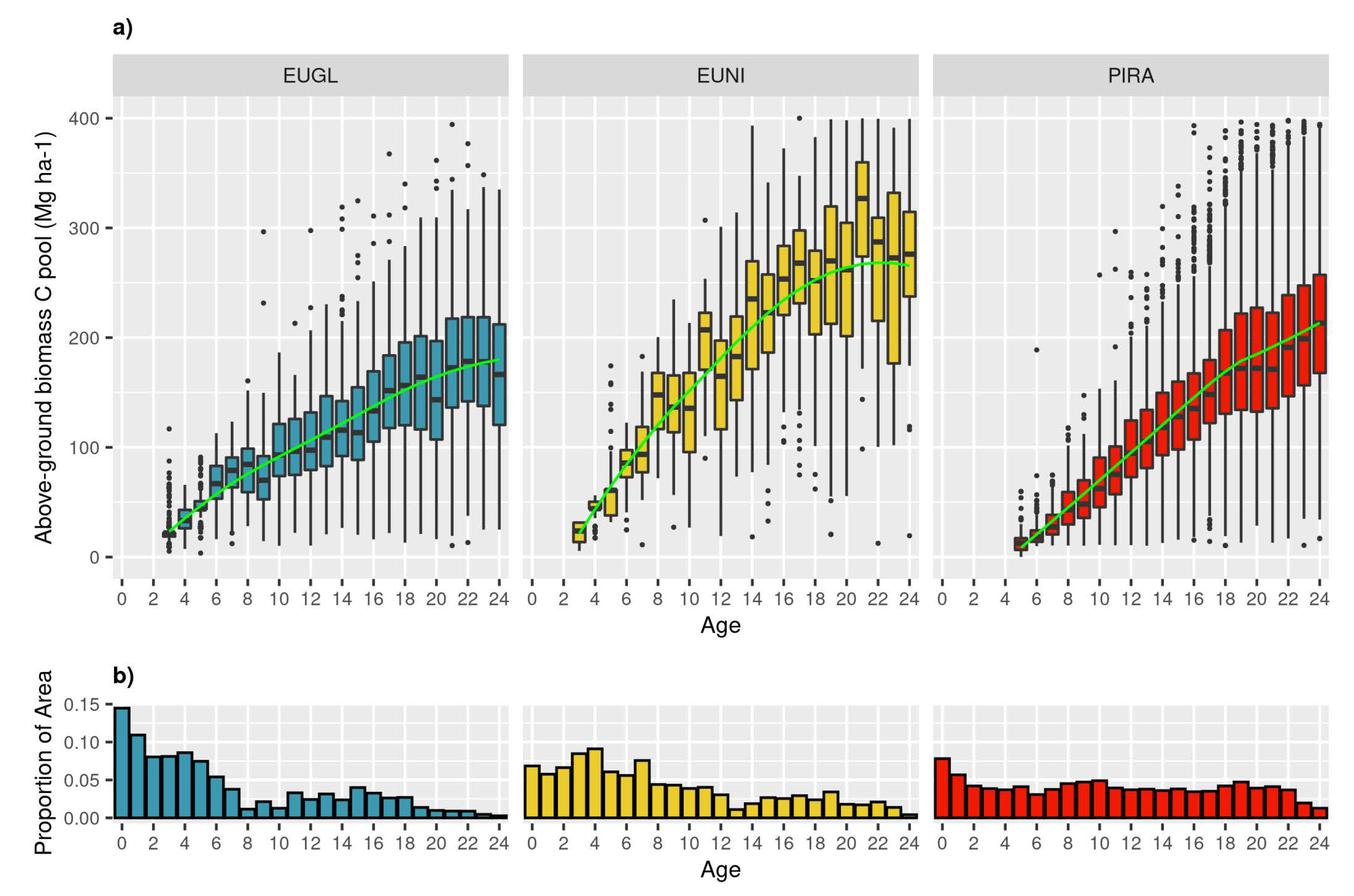
3.2. How Much C Is Present in Above-Ground Biomass at Different Ages for Different Species?

Fast-growing species in productive forest plantations have a rapid accumulation of above-ground biomass C to produce pulp or saw timber. The accumulation per unit area increases progressively over time until it reaches a maximum co-occurring with the maximum leaf area of the stand, then declines [67] this maximum varies with species and growth conditions of the site. The high variability observed in Figure 6 results from differences in site conditions and disturbance among stands. E. nitens accumulates above-ground biomass most rapidly of the three species, but appears to slow biomass growth much earlier than the other two species. At 10 years-old, the mean value of above-ground biomass C for EUGL is 93.7 Mg · ha 1 , 150.9 Mg · ha 1 for EUNI and 68.6 Mg · ha 1 for PIRA. At 20 years of age, mean values are 158.1, 292.0 and 163.1 Mg · ha 1 for EUGL, EUNI and PIRA, respectively. The current economic rotation for PIRA is 22–24 years and 12 years for EUGL and EUNI, but biomass and C accumulation continues to increase after the end of the economic rotation. Regarding the proportion of area for each age class, there is a big area with plantations with less than 1 year. The proportion of area decreases after rotation age (20–24 years for PIRA, 10–14 for EUGL and EUNI). Albeit the proportion of area from 0–2 for EUGL and EUNI and 0–4 years for PIRA is significant, commercial measures of wood volume are considered 0.

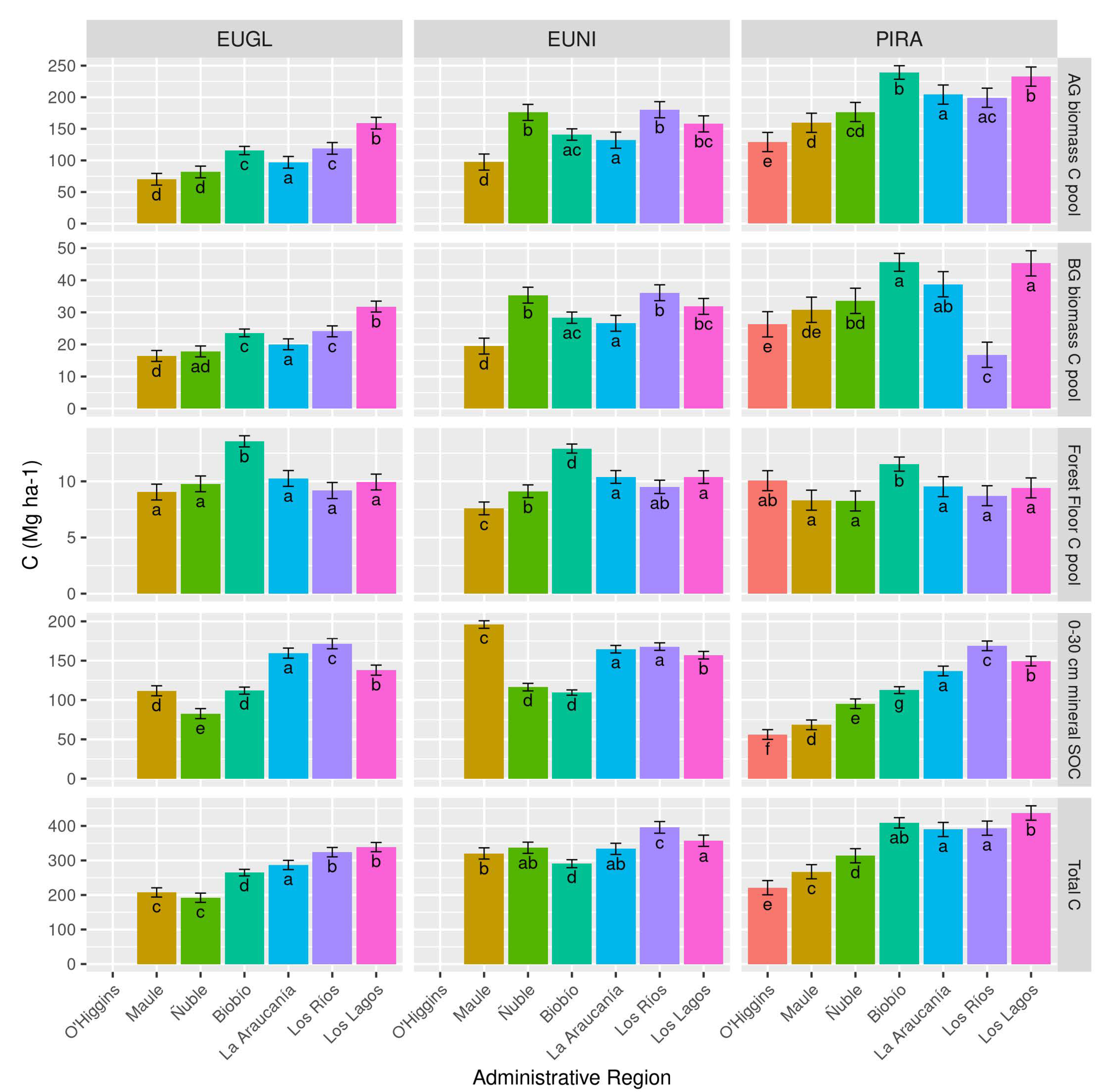
3.3. What Is the Capacity of Forest Plantations to Store C across the Different Forest Regions of Chile?

We evaluated the capacity to store C using total ecosystem C at current economic rotation ages (20–24 years for PIRA and 10–14 years for EUNI and EUGL). For the seven geographic regions evaluated, total ecosystem C stocks at rotation age ranged between 192 and 437 Mg · ha 1 . The lowest values were found in Maule and Ñuble region for EUGL, Biobío for EUNI, and O’Higgins region for PIRA. Highest values were found in Los Lagos, and Los Ríos region for EUGL, Los Ríos regions for EUNI, and Los Lagos and Biobío for PIRA (Figure 7).
Above-ground biomass C pool for EUGL has the highest value at Los Lagos regions with values around 159.0 Mg · ha 1 , followed by Biobío and Los Ríos regions (115.7 and 119.1 Mg · ha 1 ), and with the lowest and without differences for Maule and Ñuble regions (70.2 and 81.7 Mg · ha 1 , respectively). For EUNI, the highest values were found for Ñuble and Los Ríos regions (176.0 and 180.2 Mg · ha 1 ) followed by Los Lagos region (157.8 Mg · ha 1 ), and the lowest at Maule (97.4 Mg · ha 1 , respectively). For PIRA, lowest value was found at the northernmost region, O’Higgins (129.2 Mg · ha 1 ), and increasing to the south, with maximum values at Biobío (239.2 Mg · ha 1 ) and Los Lagos (232.7 Mg · ha 1 ).
For the 0–30 cm soil organic C pool, we found a similar trend for the three species analyzed. The lowest values correspond to the northern regions were mean annual temperatures are higher and precipitations are lower, with values around 100 Mg · ha 1 for EUGL and EUNI and 70 Mg · ha 1 for PIRA. At different behavior was found for plantations at Maule region shows low values for PIRA (68.4 Mg · ha 1 ), and high values for EUNI and EUGL (195.9 and 111.7 Mg · ha 1 ). The region with the biggest stock was Los Ríos and the same for the three species, with values around 170 Mg · ha 1 . However, for EUNI, Maule presents higher values than Los Ríos reaching 195.9 Mg · ha 1 .

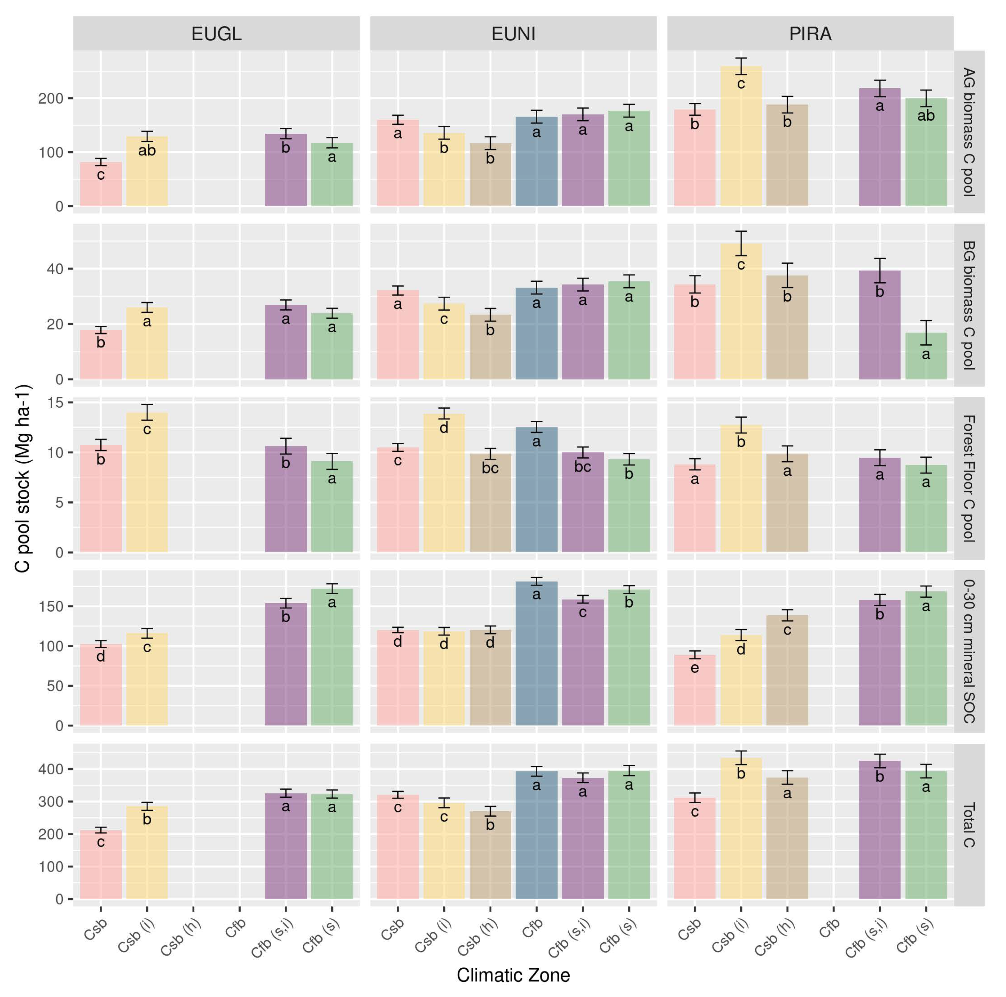
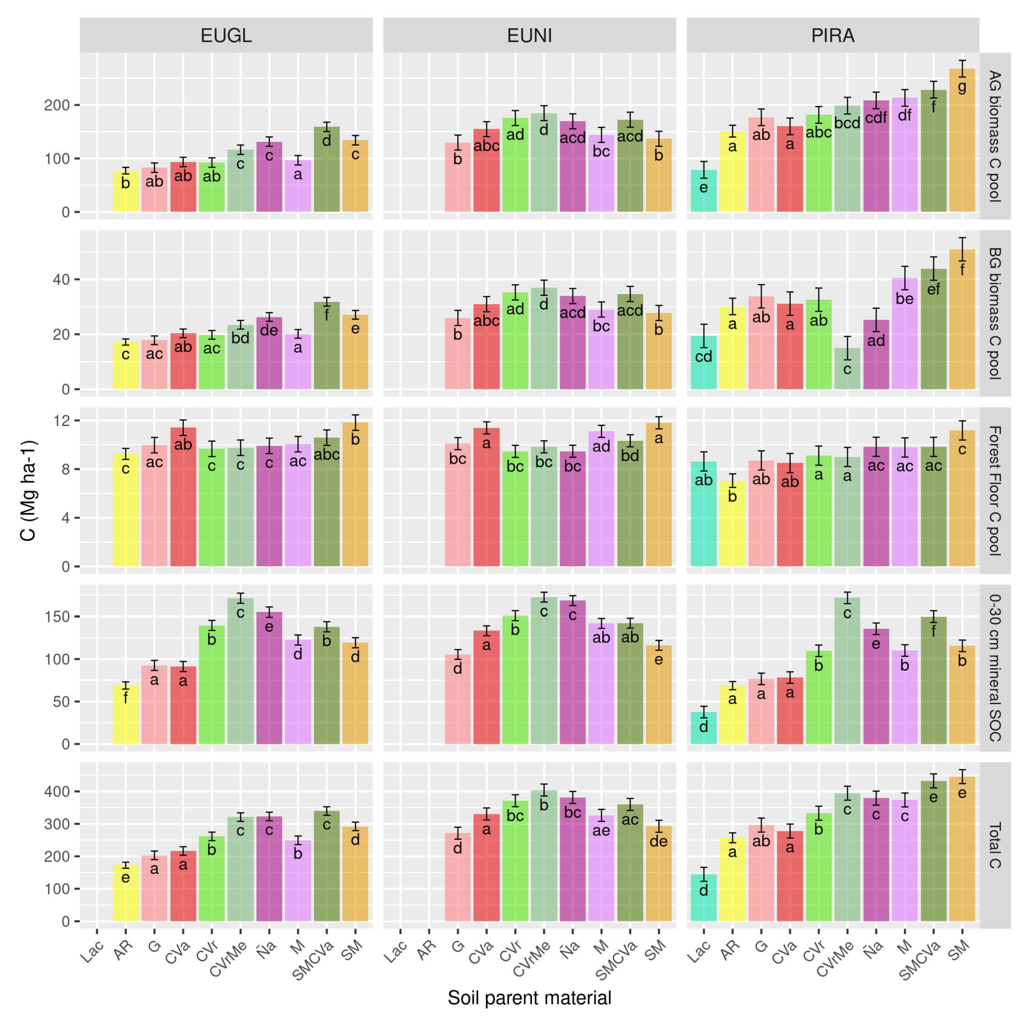
3.4. How Does This Change with Climate and Soil Types?

Total ecosystem C stocks for forests at rotation age (20–24 years for PIRA, 10–14 for EUGL and EUNI) was higher for the zones with Ocean climate (Cfb, Cfb(s), Cfb(s,i)) than the zones with a Mediterranean warm, cool summer climate (Csb, Csb(h), (Csb(i)) for all species. For PIRA, C in a Mediterranean warm, coastal influence climate (Csb(i)) has similar values than the areas with Ocean climate (Cfb, Cfb(s), Cfb(s,i)) (Figure 8).
The above-ground biomass C pool showed a different pattern than that for total C. For EUGL, the highest above-ground biomass C was found in the Cfb (s,i) and Csb (i) climates. The lowest value, 81.8 Mg · ha 1 , was found in the Mediterranean warm/cool summer climate (Csb). For EUNI, above-ground biomass C was similar for all climatic zones, with statistical differences and higher values at Csb, Cfb, Cfb(s,i), Cfb(s) compared to Csb(i) and Csb(h). For PIRA, above-ground biomass C was similar across most climate zones (179.4–218.1 Mg · ha 1 ), with higher C (259.1 Mg · ha 1 ) in the Mediterranean warm climate with a more pronounced coastal influence (Csb(i)).
The 0–30 cm soil organic C pool showed a clear trend with climate zone for all three species. The three zones with ocean climate (Cfb, Cfb(s), Cfb(s,i)), showed significantly higher values than the zones with Mediterranean climate (Csb, Csb(i), Csb(h)) (153.8–181.2 Mg · ha 1 versus 88.9–138.6 Mg · ha 1 , respectively). For all three species, the highest soil organic C value was found for the area with Ocean climate with a dry summer (Cfb(s)), with values of 172.2, 170.9 and 168.4 Mg · ha 1 for EUGL, EUNI, and PIRA, respectively, and the lowest value was found in a Mediterranean warm/cool summer climate (Csb) for EUGL (102.4 Mg · ha 1 ) and PIRA (88.9 Mg · ha 1 ). For EUNI the lowest value was similar both in this zone (120.1 Mg · ha 1 ) and in the two other Mediterranean warm climate (Csb(i) and Csb(h)) (118.1 and 120.3 Mg · ha 1 ). EUNI, the only specie with data in Ocean climate (Cfb), presented there the highest value for 0–30 cm mineral soil organic C pool with 181.2 Mg · ha 1 .
The total ecosystem C pool varied with soil parent material. For EUGL plantations, total C was highest in old volcanic ash over marine sediment (SMCVa) parent materials (339.5 Mg · ha 1 ), but with no differences with recent volcanic ash over metamorphic rock (CVrMe) and ñadi (Ña) (320.8 and 322.7 Mg · ha 1 ). For EUNI, the highest value was observed for recent volcanic ash over metamorphic rock (CVrME) (404.0 Mg · ha 1 ), also with no differences with Ñadis and recent volcanic ash (Ña and CVr) (381.3 and 371.2 Mg · ha 1 ). For PIRA, highest values were observed for marine sediment and old volcanic ash over marine sediment (SM and SMCVa) (445.4 and 432.3 Mg · ha 1 ). The lowest values were observed in sandy alluvial (AR) parent material for EUGL (172.5 Mg · ha 1 ), in granitic and marine sediment (G and SM) parent material for EUNI (271.2 and 292.5 Mg · ha 1 ), and in lacustrine (Lac) parent material for PIRA (144.4 Mg · ha 1 ) (Figure 9). The variability of 0–30 cm soil carbon with soil parent material are similar for all species, with recent volcanic ash over metamorphic rock (CVrMe) soils having the highest values (171.3, 172.6, 171.7 Mg · ha 1 for EUGL, EUNI and PIRA), followed by ñadis (Ña) soils. However, for PIRA, the second highest value was found for old volcanic ash over marine sediment (SMCVa) soils. The lowest values were observed in lacustrine (Lac) parent material (37.6 Mg · ha 1 for PIRA), in soils with sandy alluvial (AR) parent material (68.9 Mg · ha 1 ) for EUGL and in granitic soils (G) for EUNI (105.4 Mg · ha 1 ). For EUGL, the highest values of the above-ground biomass C pool were observed at old volcanic ash over marine sediment (SMCVa) (159.1 Mg · ha 1 ), and the lowest values at sandy alluvial, granitic, old volcanic ash, and recent volcanic ash soils (AR, G, CVa, and CVr) (77.2, 82.8, 93.4 and 92.3 Mg · ha 1 ). EUNI plantations showed highest and similar values for 4 soil parent materials: recent volcanic ash, recent volcanic ash over metamorphic rock, ñadis and old volcanic ash over marine sediment (CVr, CVrME, Ña, SMCVa) soils (175.6, 184.7, 169.5, and 172.5 Mg · ha 1 , respectively). And the lowest values were observed at granitic and marine sediment (G and SM) (129.8 and 136.8 Mg · ha 1 ). For PIRA, the highest value of above-ground biomass C was observed for the marine sediment (SM) parent material (267.8 Mg · ha 1 ) and the lowest at soil formed over lacustrine (Lac) parent material (78.8 Mg · ha 1 ).

4. Discussion

Our study shows that plantation forests in Chile store large amounts or carbon. The planted species differ in their C accumulation rate, with both Eucalyptus species accumulating carbon at a more rapid rate than radiata pine with the most rapid C accumulation for E. nitens. These differences indicate that management changes could impact plantation C storage by changing the species mix and/or the rotation length. There are large differences in above-ground biomass C by species, administrative region, climate and soil parent material, with faster C accumulation and higher biomass and soil C in the cooler, wetter areas in the southern regions on fertile soils derived from volcanic ash. A detailed discussion of these differences is given below, together with a comparison of the data from this study with that used in [34].

4.1. The Capacity of Forests to Store Carbon by Species

The capacity of PIRA to store C in above-ground biomass in this study is similar to that reported for other studies. In New Zealand, Oliver et al. [68] reported 79.4 and 105.6 Mg · ha 1 for two stands of 15 and 16 years old, similar to the ones reported here, where the interquartile range for PIRA at age 15 was 80.3 to 124.7 Mg · ha 1 , and for age 16 was 84.4 to 137.7 Mg · ha 1 . Oliver et al. [68] also reported a value for C stored in the soil organic layer (forest floor) for the same stands of 13.7 to 14.6 Mg · ha 1 , slightly higher than the value reported by us of 9.8 ± 0.5 Mg · ha 1 . Guo et al. [69] reported 71.6 Mg · ha 1 for soil organic C up to 1 m, 8.0 Mg · ha 1 for the soil organic layer (forest floor), and 95.0 Mg · ha 1 for above-ground biomass in a 16-years-old PIRA plantation in Australia. In Mozambique, Guedes et al. [70], reported 162.1 ± 64.0 Mg · ha 1 for above-ground biomass C, 53.3 ± 17.7 Mg · ha 1 for below-ground biomass C, 12.1 ± 5.6 Mg · ha 1 for the soil organic layer (forest floor) C and 135.2 ± 51.1 Mg · ha 1 for soil organic C, for plantations of Pinus at rotation age (34 years). Balboa-Murias et al. [71] assessed the temporal dynamics of C stored in above-ground tree biomass in even-aged, pure stands of maritime pine and radiata pine managed under different silvicultural regimes in northwest Spain. Total above-ground carbon storage for the whole 30 years rotation in radiata pine plantations (clear-cutting plus thinning) ranged between 96.0 Mg · ha 1 and 187.0 Mg · ha 1 for different initial tree density and site quality. In the same region [72] reported total live C stocks in above and below ground live biomass of radiata pine plantations at 11 years old in an experimental design for silvopastoral systems of 130.69 ± 9.68 and 145.80 ± 27.21 Mg · ha 1 , depending on the initial tree density.
Soares and Tomé [73] in a EUGL fertilization-irrigation experiment in Portugal estimated above-ground biomass for 6-year-old plantations of 93.66–157.42 Mg DM · ha 1 (47.46–80.28 Mg C · ha 1 ) and below-ground biomass (roots) of 25.88–44.16 Mg DM · ha 1 (13.19–22.52 Mg C · ha 1 ). The normal rotation for EUGL in Portugal is 10-12 years. Demessie et al. [74] measured biomass on EUGL plantations in southern Ethiopia, showing total C in above-ground biomass of 493 ± 106.01 Mg · ha 1 and SOC in the range of 175.5 ± 13.62 Mg · ha 1 at 22 years old. In Mozambique, Guedes et al. [70], reported 202.5 ± 124.6 Mg · ha 1 for above-ground biomass C, 58.7 ± 31.0 Mg · ha 1 for below-ground biomass C, 6.6 ± 3.1 Mg · ha 1 for the soil organic layer (forest floor) C and 138.8 ± 60.2 Mg · ha 1 for soil organic C, for plantations of Eucalyptus at rotation age.
In Chile, research on the carbon content in forest plantations is scarce. Within these, Espinosa et al. [24] estimated that the C content in PIRA stems would average 55 Mg C· ha 1 , and Acuña et al. [75] reports values between 6.1–6.9 Mg C · ha 1 for PIRA harvest residue (leaves, twigs, branches and unmerchantable stems). Values more consistent with our estimates are found in the reports of the Bioenercel Consortium, that conducted research on biofuels from woody material [76]. This consortium estimated biomass C content using destructive sampling in the Ñuble, Biobío and Araucanía regions, estimating the total above-ground biomass C of PIRA of 62.6 Mg · ha 1 (42.5–151) in sandy alluvial soils, 139.6 Mg · ha 1 (124–157.5) in soils from recent volcanic ash, and 183.7 Mg · ha 1 (129–251.5) in marine sediment soils for stands 15–31 years old. The Consortium estimated above-ground biomass C of 13–16 year-old EUGL as 100.1 Mg · ha 1 (46–178), and of 15–19 year-old EUNI at 271.2 Mg · ha 1 (225.5–306), also with destructive sampling. The results presented in [76] are similar to those found in our study. For PIRA, we found 102.5 and 213.0 Mg C · ha 1 at 13 and 24 years old, respectively. EUGL biomass averaged 115.6 and 139.2 Mg C · ha 1 in our study at ages 13 and 16 years old, respectively. EUNI biomass averaged 227.4 and 277.2 Mg C · ha 1 in our study at ages 15 and 19 years old, respectively. Small differences between the Bioenercel values and those of our study may be due to the Bioenercel estimates being from a smaller geographic area and not the larger longitudinal range evaluated in this article.
As shown in Figure 4, the above-ground C stock at rotation age differed by species, with PIRA having with the highest value, followed by EUNI and them EUGL. Because this comparison is for different ages for each species, the results differ if we compare at the same age. As we presented in Section 3.2 and Figure 6, at 10 years old, above-ground C pool was largest for EUNI followed by EUGL, with PIRA having the lowest value. At 20 years-old, above ground biomass is greatest in EUNI, with lower and similar values for EUGL and PIRA, although there are few stands of EUGL at that age.
The growth of an even-aged forest plantation has different development stages [40,77], and the dynamics of above-ground C vary with stand development and age. Figure 6 shows that PIRA and EUNI both have slower C accumulation after age 16, with growth slowing less or not slowing for EUGL. Figure 6 also shows that while the accumulation rate slows for older stands, carbon storage continues to increase after age 20 years, especially for PIRA. Even though the proportion of older stands is low across the landscape, these stands are especially important for storing C and C will likely continue to accumulate in them after age 20–24 years. Among the three species, EUNI accumulates C the most quickly, followed by EUGL and finally PIRA. C accumulation in PIRA is reduced by pruning and thinning that reduce its annual accumulation rate, while EUGL and EUNI are not thinned or pruned.
At the global scale, the importance of above-ground biomass and its capacity to store carbon has been well researched and quantified [78]. Soil carbon storage, while very important [79], still has large uncertainties [80,81]. Scharlemann et al. [20] summarized global data and reported a proportion of soil C to total C as 50 to more than 75% for this region. The value for this study is between 29–41% (Figure 5) but this study’s lower proportions arise from our study estimating only 0 to 30 cm of depth compared to 0–100 cm for the global synthesis. According to [20] topsoil C (0–30 cm) represents between 46–65% of the total soil organic C, with differences in different climatic regions. Soil formed from volcanic materials represent an important part of our study, and these soils contain more SOC than other soil types, particularly at depths below 1 m [82]. For other volcanic ash soil in Washington USA sampled to 3 m depth, (58.2%) of SOC was located below 30 cm [83]. These results and those of Scharlemann et al. [20] suggest that quantifying soil C below 30 cm for our study sites would be an important priority for future research.

4.2. The Capacity of Forests to Store Carbon in Different Regions

When comparing the different administrative regions, the amount of biomass increases from north to south for all species (Figure 7). Maximum C storage for PIRA is observed in the Biobío region with high productivity in SM soils together with a Csb(i) climate with moderate temperatures and with abundant precipitation. For EUNI, the Ñuble region has the highest biomass production because the plantations are located in high productivity CVr soils, towards the foothills with lower temperatures and greater precipitation (Figure 2 and Figure 3). 0–30 cm soil C also increases from north to south, where Cfb climate conditions are more humid and with lower temperatures. In the north, climate is warmer and drier, productivity and litter inputs to soils are lower and soils are more degraded.
We can also compare this study’s regional differences with estimates from the National Forest Institute (INFOR) national inventory that is used to forecast wood availability for the main tree species. The most recent report, [37], summarizes planting areas, stand management and forest yield, and this information can be used to estimate above-ground C stocks by region. We used data about mean annual increments in [37] grouped by Growth Areas (GA), Site Class, and Management Schemes to compare with our values by region.
We related Growth areas to region as follows: GA 1: Coastal dry land in the O’Higgins region and interior dry land in the Maule region; GA 2: Coastal dry land in the Maule region and north coastal zone in the Biobío region; GA 4: Pre-mountainous sector of the Maule, Biobío and La Araucanía regions; GA 5: Sandy area between the Itata river, south of the San Carlos de Purén sector to the southern bank of the Biobío river; GA 6: Coastal zone of the Biobío region and northern part of the Araucanía region; GA 7: Inland zone of the Biobío region and northern part of the Araucanía region, between the Itata river and the Traiguén zone; GA 9: Coastal zone of the Araucanía region to the south of Purranque, considering the coastal zone in the north and including the central zone in the Los Ríos and Los Lagos region. GA 3 and 8 do not have forest plantations. The Site Class corresponds to a productivity rating of 1 (high) to 4 (low) (Table A2). Values reported in this study are similar to those estimated from data in the Buchner et al. [37], considering the difficulty of matching Growth Area to region. Our value for PIRA in the Biobío region is 4.7% greater than that reported for GA4 and GA6 (Figure 7). The range of values reported for GA5 (36.7–100.0 Mg · ha 1 ) is lower than the value we report for AR soils (141.0 Mg · ha 1 ) (Table A6) for PIRA. For EUGL the value reported here, 68.1 Mg · ha 1 , is between the range reported in the INFOR report (56.4–96.8 Mg · ha 1 ). Our study found low values in the south of the Maule region, coinciding with Lac soils (71.0 Mg · ha 1 ) (Figure 3b) compared with the lowest value for that area in the INFOR report of 68.5 Mg · ha 1 .
Recently, Heilmayr et al. [34] evaluated the impact of subsidies on plantation expansion by using an econometric land use change model. To estimate the carbon impact of the plantations, the authors assumed a regulated forest estate (the same amount of area for every age class) together with literature values of biomass volume for every administrative region of Chile. Then, wood volume was converted to carbon density using an approach similar to the one used in this study, but with different coefficients (Equation (1), Table 1). Aggregated regional carbon density was calculated using the area of plantations for a given species (PIRA, EUGL, EUNI) as a percent of all plantations [34,84]. If we use the same procedure as in [34], assume a regulated forest with current rotation ages that vary with species, and produce a weighted carbon density per region, our estimates were much larger than the carbon densities presented in [84]. Our value for EUGL for a regulated forest is 32% higher in the Maule region (35.1 to 26.6 Mg · ha 1 ), and 57%, 33%, 64% an 86% higher for Biobío, La Araucanía, Los Ríos and Los Lagos regions (Table A4). These discrepancies are much higher for the other species: 148% higher for PIRA in the O’Higgins region (61.4 to 24.71 Mg · ha 1 ), 174% and 191% for EUNI and PIRA in Maule, 180% and 204%; 138% and 210%; 147% and 141%; 95% and 164% higher for EUNI and PIRA for Biobío, La Araucanía, Los Ríos and Los Lagos regions. When comparing with the share area of each species as reported by Gysling Caselli et al. [85], the discrepancies remain large. Our combined value is 189% higher than the proposed for Maule region (77.12 to 26.63 Mg · ha 1 ); 194% higher for Biobío (92.3 to 31.3 Mg · ha 1 ); 177% higher for La Araucanía region (85.1 to 30.7 Mg · ha 1 ); 143% higher for Los Ríos region (91.12 to 37.3 Mg · ha 1 ) and 109% higher for Los Lagos region (77.27 to 36.89 Mg · ha 1 ).
Because our approach and the approach used in Heilmayr et al. [34] was the same, but the coefficients used to convert volume to carbon density were different, the differences might be caused by the different coefficients. However, the differences in the coefficients would only account for differences of 20 to 30%. For example, for a plantation of PIRA with 100 m 3 of merchantable wood volume, the coefficients applied by Heilmayr et al. [34] produce a value of 27.3, those suggested by Aalde et al. [17] estimate a value 35.7 Mg or 30%, which is less than the observed differences of 140 to 210%. Doing the same exercise with a plantation of EUGL or EUNI and considering 75 m 3 of merchantable wood volume, the differences are of 20%, again less than the observed differences of 32 to 86% for EUGL or 95 to 180% for EUNI. The difference between our approach and that of Heilmayr et al. [34] is that our results are based on a country-wide inventory of tree volume and those of Heilmayr et al. [34] are based on older estimates from the literature with limited sampling.

4.3. The Capacity of Forests to Store Carbon in Different Climatic Zones

The Chilean territory is characterized by its climatic and topographic variability, where precipitation, temperature and soil are the factors that determine productivity [86]. Above-ground C stock potential is strongly correlated with the amount of light interception or leaf Area Index (LAI) [86,87] and LAI depends on several factors such as: suitable selection of species, crop design (initial stock density and rotation), management regimes (weed control, fertilization, irrigation); and climatic conditions [88,89]. The variability in the accumulation of carbon at the landscape level is a function of the prevailing edaphoclimatic characteristics at each site. In Chilean soils, SOC stocks increased with latitude [90]. PIRA is a species capable of developing in a wide variety of Chilean environments. Because of its environmental plasticity, PIRA was subsidized for establishment over a vast area of southern Chile [91]. Across its wide range it Chile, its productivity is determined by nutritional factors [91] and precipitation [86]. On the other hand, the number of cold days within a year (temperature below 0 °C) plays an important role in the distribution of species of Eucalyptus. EUGL plantations are established in areas where this environmental factor does not affect their survival rate. Other areas with temperatures below this threshold are planted with EUNI plantations. Studies such as those developed by [87,92,93] show that temperature and water stress are the two factors that negatively impact the LAI of the genus Eucalyptus, which translates into a poor accumulation of carbon in places that limit temperature and precipitation.
Figure 8 shows that in the O’Higgins and Ñuble regions in north-central of Chile, the carbon pool is significantly less than in the rest of the regions (from Biobío to Los Lagos). In this area, the climate is extremely dry in summer, rainy seasons do not exceed 4 months, and high temperatures during summer allow only limited biomass production. EUNI grows better in these regions than the other two species because EUNI plantations are in the foothills above 750 m a.s.l., in conditions more related to climate Csb(h), while the other two species are not. The Csb(i) climate is a coastal climate that is moderated by the humid ocean winds in the summer, with an annual amplitude less than 5 °C. It is a mild climate for the development of biomass in the plantations, favoring a productivity that equals or exceeds the productivities found in more humid climates such as those found in Cfb climates.
We found that the values for topsoil organic C were higher in the 3 zones with Cfb climate (i.e., Cfb, Cfb (s,i), Cfb(s)), which coincides with areas of higher precipitation and lower annual temperature (Figure 2 and Figure 8). Comparing the regions with Mediterranean climate (Csb, Csb(i), Csb(h)), it is observed that the values are higher in the areas with coastal influence, with the highest water availability in that area.

4.4. The Capacity of Forests to Store Carbon in Different Soils

Our results showed a positive relation between 0–30 cm soil carbon and moisture regime and variability of soil carbon with soil parent material. Volcanic soils in Chile store the most soil C [94], even though land use change and management can alter soil properties [95]. Reyes Rojas et al. [45] estimated that forests in central Chile contained larger amounts of soil carbon on volcanic soils, especially under moist regimes. The poorest sites are those with Lac parent material located to the north of the central valley, where PIRA can grow, but only slowly. Here, past agricultural activities (rice or wheat crops) caused soil erosion and current soil bulk density (>1.2 g · cm 3 ) makes agricultural production difficult (Figure 2 and Figure 9) [96,97]. Poor sites for soil carbon are also found in sandy alluvial soils of AR parent material. Low biomass production and low above-ground biomass C in this soil, coupled with the low capacity of these soils to accumulate SOC and store water within the soil profile leads to low soil C stocks. The more clayey volcanic soils store more soil C [35]. Soils formed over SM (SM and SMCVa) correspond to highly productive soils for PIRA and EUGL, given their structure and depth that favour root development and resource availability.
Compared to EUGL, EUNI is a higher yielding species planted on highly productive sites where growth of EUGL is limited by low temperatures, frost and excess soil water [87,98,99,100]. This is why EUNI achieves high biomass in soils of CVr and CVrMe origin in the foothills and coastal areas, which have good structure, but where there are cold and windy conditions and frost events. EUNI also good performance in soils of Ña origin, which are shallow soils of recent volcanic origin, have high SOC, but contain an iron-cemented layer [66,101], which must be ripped to ensure the establishment of EUNI. CVrMe soils have more soil C for all 3 species, because these soils are located in the Los Ríos and Los Lagos regions, where temperatures are lower and organic matter decomposition is likely slower. High soil C in 0–30 cm is also found in soils of Ña origin. Areas with these soils also have lower temperatures and water saturation of soil, both factors that may slow decomposition. Soil C is greater in EUNI plantations for all the types of parental material compared to the other two species. Soil C may accumulate at a higher rate for EUNI because of its greater productivity and likely greater detrital production and also because EUNI is preferred for colder sites where decomposition may be slower.

5. Conclusions

Across the plantation landscape of 2,197,386 ha from the O’Higgins region (latitude 35°14′) to the Los Lagos region (latitude 40°6′) total carbon averaged 322.4 Mg · ha 1 , 343.4 Mg · ha 1 for Pinus radiata, 351.9 Mg · ha 1 for Eucalyptus nitens and 254.6 Mg · ha 1 for E. globulus. Total C storage in plantation forests and their soils is 708 Tg. This compares to the annual fossil fuel C emissions for Chile in 2019 of 23 million tonnes C (=23 × 10 12 g or 23 Tg) [102]. The data compiled and the procedures used in this study provide a forest carbon baseline and database for assessing changes in future studies. The collaborative effort and public-private data sharing also point the way towards how future C assessments can be accomplished. The baseline data will be valuable for modelling C storage changes under different management regimes (changes in species, rotation length and stocking) and for different future climates.

Author Contributions

Conceptualization, G.F.O., B.B.-K. and M.G.R.; Data curation, B.B.-K. and F.G.; Formal analysis, G.F.O. and C.R.M.; Funding acquisition, G.F.O. and B.B.-K.; Methodology, G.F.O., M.G. and H.G.; Visualization, G.F.O., F.G. and M.G.R.; Writing—original draft, G.F.O., M.G., H.G., C.R.M. and B.B.-K.; Writing—review & editing, E.C.A., P.M.-Q., E.A., H.E.B. and M.G.R. All authors have read and agreed to the published version of the manuscript.

Funding

This research received no external funding.

Acknowledgments

We want to acknowledge Rodrigo Sobarzo and Fernando Bustamante from Forestal Arauco for preparing and providing the merchantable volume database.

Conflicts of Interest

The authors declare no conflict of interest. The funders had no role in the design of the study; in the collection, analyses, or interpretation of data; in the writing of the manuscript, or in the decision to publish the results.

Appendix A. Environmental Covariates Used in Digital Soil Mapping

Table A1. Enviromental covariates used to model soil organic carbon and forest floor carbon using digital soil mapping techniques.
CategorySourceResolutionVariables
TopographySRTM90 mElevation model, Aspect, Slope, Chanel Network Base Level, Channel Network Distance, Longitudinal Curvature, Convergence Index, Slope Length and Steepness Factor, Maximal Curvature, Minimal Curvature, Profile Curvature, Tangential Curvature, Terrain Surface Convexity, Terrain ruggedness index, Topographic Position Index, Topographic Wetness Index, Valley Depth
ClimateCR2-Uchile500 mMean annual temperature, Mean diurnal range (mean of max temp-min temp), Isothermality, Temperature seasonality, Max temperature of warmest month, Min temperature of coldest month, Temperature annual range, Mean temperature of the wettest quarter, Mean temperature of driest quarter, Mean temperature of warmest quarter, Mean temperature of coldest quarter, Total (annual) precipitation, Precipitation of wettest month, Precipitation of driest month, Precipitation seasonality, Precipitation of wettest quarter, Precipitation of driest quarter, Precipitation of warmest quarter, Precipitation of coldest quarter, average number of cold Day
Soil MorphologyCIREN90 mParent Material
Vegetation indicesMODIS250 mAverage Enhance vegetation index from last 20 years, Minimum Enhance vegetation index, Maximum Enhance vegetation index, Enhanced vegetation index range, Standard deviation for EVI from last 20 years

Appendix B. INFOR Reference Values

Table A2. Above-ground Biomass Carbon Pool for the different Growth Areas, Site Class and Management Scheme (1–10 for Pinus radiata, 11 Eucalyptus globulus and 12 Eucalyptus nitens). Rotation length is 20 years for management scheme 1, 22 years for 2 and 3, 24 for 7 to 10, and 12 years for management scheme 11 and 12. Above-ground Biomass Carbon calculated using the methodology presented in Section 2.2 and data from [37].
Growth AreaSite ClassManagement Scheme
123789101112
11207.1188.5180.6179.9171.4162.8171.460.592.2
2164.2149.2141.4145.751.4128.5137.164.578.6
3121.4110.0102.1102.8102.894.2102.848.472.6
485.778.570.768.568.568.577.140.366.5
21214.2212.1196.3197.1188.5179.9197.196.887.6
2178.5164.9157.1154.2154.2145.7154.266.582.9
3142.8141.4125.7128.5128.5120.0128.564.596.8
4107.194.286.485.785.777.194.264.596.8
41228.5204.2196.3179.9179.9154.2188.596.8170.5
2178.5157.1141.4128.5137.1128.5137.1101.4147.5
3149.9133.5125.7120.0111.4102.8102.882.9119.8
4121.4102.1102.185.777.185.794.296.892.2
51100.086.478.577.177.168.577.187.696.8
278.570.762.860.060.060.060.096.882.9
364.355.047.151.451.442.851.466.584.7
450.039.339.336.736.742.842.856.466.5
61221.3204.2188.5188.5179.9154.2188.5142.8198.1
2171.4157.1141.4137.1137.1128.5145.7129.0165.9
3142.8125.7117.8145.7120.0102.8120.0115.2129.0
4107.194.286.485.785.777.185.782.996.8
71207.1196.3188.5179.9179.9171.4179.9101.4165.9
2178.5164.9157.1154.2154.2137.1154.282.9147.5
3149.9141.4133.5128.5128.5120.0128.596.8115.2
4114.2102.1102.194.294.285.794.266.578.3
91214.2188.5172.8171.4162.8154.2171.4110.6198.1
2164.2141.4133.5120.0120.0120.0128.596.8175.1
3121.4110.0102.194.294.285.794.278.3152.1
492.878.570.760.060.060.060.084.7115.2

Appendix C. Average C Stock Values of the Different Pool Per Specie, Region, Climatic Zones and Parent Material

Table A3. Average (±standard deviation, n = 11,084) carbon (C) stocks [Mg · ha 1 ] in each specie at rotation age (10–14 years-old for EUGL and EUNI, 20–24 years-old for PIRA).
SpecieAgeAbove-Ground
Biomass C
Below-Ground
Biomass C
Forest
Floor C
Soil Organic
C (0–30 cm)
Total
Ecosystem C
EUGL10–14105.9 ± 5.622.0 ± 1.212.0 ± 0.4115.2 ± 3.4254.6 ± 8.5
EUNI10–14164.7 ± 8.033.0 ± 1.710.5 ± 0.5146.0 ± 4.9351.9 ± 12.3
PIRA20–24196.8 ± 8.036.2 ± 1.79.6 ± 0.5100.7 ± 4.9343.4 ± 12.1
Table A4. Average (±standard deviation, n = 11,084) carbon stocks [Mg · ha 1 ] for each administrative region for each specie at rotation age (10–14 years-old for EUGL and EUNI, 20–24 years-old for PIRA).
SpecieAdministrative
Region
Above-Ground
Biomass C
Below-Ground
Biomass C
Forest
Floor C
Soil Organic
C (0–30 cm)
Total
Ecosystem C
EUGLMaule70.2 ± 4.716.4 ± 0.99.0 ± 0.4111.7 ± 3.3207.4 ± 6.9
Ñuble81.7 ± 4.717.8 ± 0.99.8 ± 0.482.7 ± 3.3192.0 ± 6.9
Biobío115.7 ± 3.423.6 ± 0.613.6 ± 0.3111.9 ± 2.3264.7 ± 4.9
La Araucanía97.0 ± 4.720.0 ± 0.910.3 ± 0.4159.6 ± 3.3286.9 ± 6.9
Los Ríos119.1 ± 4.724.1 ± 0.99.2 ± 0.4171.5 ± 3.3324.0 ± 7.0
Los Lagos159.0 ± 4.731.8 ± 0.99.9 ± 0.4138.0 ± 3.3338.7 ± 6.9
EUNIMaule97.4 ± 6.519.5 ± 1.37.6 ± 0.3195.9 ± 2.5320.4 ± 8.3
Ñuble176.0 ± 6.535.3 ± 1.39.1 ± 0.3116.3 ± 2.5336.8 ± 8.3
Biobío141.0 ± 4.628.3 ± 0.912.9 ± 0.2109.4 ± 1.7290.6 ± 5.9
La Araucanía132.0 ± 6.526.6 ± 1.310.4 ± 0.3164.6 ± 2.5333.6 ± 8.3
Los Ríos180.2 ± 6.536.1 ± 1.39.5 ± 0.3167.9 ± 2.5395.8 ± 8.7
Los Lagos157.8 ± 6.531.9 ± 1.310.4 ± 0.3157.0 ± 2.5357.0 ± 8.3
PIRAO’Higgins129.2 ± 7.826.3 ± 2.010.1 ± 0.556.1 ± 3.2221.1 ± 10.5
Maule159.6 ± 7.830.8 ± 2.08.3 ± 0.568.4 ± 3.2267.3 ± 10.5
Ñuble176.6 ± 7.833.6 ± 2.08.3 ± 0.595.2 ± 3.2313.6 ± 10.5
Biobío239.2 ± 5.545.6 ± 1.411.5 ± 0.3112.5 ± 2.2408.5 ± 7.4
La Araucanía204.2 ± 7.838.7 ± 2.09.5 ± 0.5136.9 ± 3.2389.6 ± 10.5
Los Ríos199.2 ± 7.816.8 ± 2.08.7 ± 0.5168.8 ± 3.2393.5 ± 10.5
Los Lagos232.7 ± 7.845.3 ± 2.09.4 ± 0.5149.4 ± 3.2436.8 ± 10.5
Table A5. Average (±standard deviation, n = 11,084) carbon (C) stocks [Mg · ha 1 ] in each climatic zones for each specie at rotation age (10–14 years-old for EUGL and EUNI, 20–24 years-old for PIRA).
SpecieClimatic
Zone
Above-Ground
Biomass C
Below-Ground
Biomass C
Forest
Floor C
Soil Organic
C (0–30 cm)
Total
Ecosystem C
EUGLCsb81.8 ± 3.417.8 ± 0.610.7 ± 0.3102.4 ± 2.2212.3 ± 4.5
Csb (i)129.2 ± 4.926.0 ± 0.914.0 ± 0.4115.9 ± 3.1285.2 ± 6.4
Cfb (s,i)134.4 ± 4.926.9 ± 0.910.6 ± 0.4153.8 ± 3.1325.8 ± 6.4
Cfb (s)117.5 ± 4.923.9 ± 0.99.1 ± 0.4172.2 ± 3.1323.0 ± 6.4
EUNICsb160.1 ± 4.332.1 ± 0.810.5 ± 0.2120.1 ± 1.8320.5 ± 5.4
Csb (i)136.1 ± 6.127.4 ± 1.213.9 ± 0.3118.5 ± 2.5295.9 ± 7.6
Csb (h)116.7 ± 6.123.3 ± 1.29.9 ± 0.3120.3 ± 2.5270.2 ± 7.6
Cfb165.8 ± 6.133.2 ± 1.212.5 ± 0.3181.2 ± 2.5392.7 ± 7.6
Cfb (s,i)170.1 ± 6.134.2 ± 1.210.0 ± 0.3158.7 ± 2.5373.1 ± 7.6
Cfb (s)176.9 ± 6.135.4 ± 1.29.3 ± 0.3170.9 ± 2.5395.1 ± 8.0
PIRACsb179.4 ± 5.634.3 ± 1.68.8 ± 0.388.9 ± 2.5311.6 ± 7.6
Csb (i)259.1 ± 7.949.1 ± 2.312.7 ± 0.4113.8 ± 3.6434.5 ± 10.7
Csb (h)188.0 ± 7.937.6 ± 2.39.9 ± 0.4138.6 ± 3.6374.0 ± 10.7
Cfb (s,i)218.1 ± 7.939.3 ± 2.39.5 ± 0.4157.8 ± 3.6424.7 ± 10.7
Cfb (s)199.7 ± 7.916.8 ± 2.38.7 ± 0.4168.4 ± 3.6393.6 ± 10.7
Table A6. Average (±standard deviation, n = 11,084) carbon (C) stocks [Mg · ha 1 ] in each parent material for each specie at rotation age (10–14 years-old for EUGL and EUNI, 20–24 years-old for PIRA).
SpecieSoil
Parent Material
Above-Ground
Biomass C
Below-Ground
Biomass C
Forest
Floor C
Soil Organic
C (0–30 cm)
Total
Ecosystem C
EUGLAR77.2 ± 3.217.2 ± 0.69.3 ± 0.268.9 ± 2.2172.5 ± 4.8
G82.8 ± 4.517.8 ± 0.810.0 ± 0.392.5 ± 3.0203.1 ± 6.8
CVa93.4 ± 4.520.3 ± 0.811.4 ± 0.391.2 ± 3.0216.3 ± 6.8
CVr92.3 ± 4.519.8 ± 0.89.7 ± 0.3139.6 ± 3.0261.4 ± 6.8
CVrMe116.3 ± 4.523.5 ± 0.89.8 ± 0.3171.3 ± 3.0320.8 ± 6.8
Ña131.5 ± 4.526.3 ± 0.89.9 ± 0.3155.1 ± 3.0322.7 ± 6.8
M96.7 ± 4.520.1 ± 0.810.0 ± 0.3122.4 ± 3.0249.3 ± 6.8
SMCVa159.1 ± 4.531.8 ± 0.810.6 ± 0.3138.0 ± 3.0339.5 ± 6.8
SM134.1 ± 4.527.1 ± 0.811.8 ± 0.3119.2 ± 3.0292.3 ± 6.8
EUNIG129.8 ± 7.226.0 ± 1.410.1 ± 0.3105.4 ± 3.0271.2 ± 9.5
CVa154.8 ± 7.231.0 ± 1.411.4 ± 0.3133.3 ± 3.0330.4 ± 9.5
CVr175.6 ± 7.235.2 ± 1.49.5 ± 0.3150.9 ± 3.0371.2 ± 9.5
CVrMe184.7 ± 7.236.9 ± 1.49.8 ± 0.3172.6 ± 3.0404.0 ± 9.5
Ña169.5 ± 7.233.9 ± 1.49.5 ± 0.3168.5 ± 3.0381.3 ± 9.5
M144.1 ± 7.229.0 ± 1.411.1 ± 0.3141.9 ± 3.0326.1 ± 9.5
SMCVa172.5 ± 7.234.7 ± 1.410.3 ± 0.3142.3 ± 3.0359.7 ± 9.5
SM136.8 ± 7.227.7 ± 1.411.8 ± 0.3116.1 ± 3.0292.5 ± 9.5
PIRALac78.8 ± 8.019.4 ± 2.28.6 ± 0.437.6 ± 3.5144.4 ± 11.0
AR151.1 ± 5.730.1 ± 1.57.1 ± 0.368.7 ± 2.5257.0 ± 7.8
G177.0 ± 8.033.8 ± 2.28.7 ± 0.476.6 ± 3.5296.1 ± 11.0
CVa160.0 ± 8.031.2 ± 2.28.5 ± 0.478.2 ± 3.5277.7 ± 11.0
CVr181.4 ± 8.032.6 ± 2.29.1 ± 0.4109.7 ± 3.5332.8 ± 11.0
CVrMe198.7 ± 8.014.9 ± 2.29.0 ± 0.4171.7 ± 3.5394.4 ± 11.0
Ña208.5 ± 8.025.2 ± 2.29.8 ± 0.4135.7 ± 3.5379.2 ± 11.0
M213.3 ± 8.040.5 ± 2.29.8 ± 0.4110.1 ± 3.5373.6 ± 11.0
SMCVa228.7 ± 8.043.9 ± 2.29.8 ± 0.4149.9 ± 3.5432.3 ± 11.0
SM267.8 ± 8.050.9 ± 2.211.2 ± 0.4115.5 ± 3.5445.4 ± 11.0

References

  1. Oreskes, N. The Scientific Consensus on Climate Change. Science 2005, 306, 2004–2005. [Google Scholar] [CrossRef] [PubMed] [Green Version]
  2. Stocker, T.F.; Qin, D.; Plattner, G.K.; Tignor, M.; Allen, S.K.; Boschung, J.; Nauels, A.; Xia, Y.; Bex, V.; Midgley, P.M.; et al. Climate change 2013: The physical science basis. In Contribution of Working Group I to the Fifth Assessment Report of the Intergovernmental Panel on Climate Change; Cambridge University Press: Cambridge, UK; New York, NY, USA, 2013; Volume 1535. [Google Scholar]
  3. Rosenzweig, C.; Karoly, D.; Vicarelli, M.; Neofotis, P.; Wu, Q.; Casassa, G.; Menzel, A.; Root, T.L.; Estrella, N.; Seguin, B.; et al. Attributing physical and biological impacts to anthropogenic climate change. Nature 2008, 453, 353–357. [Google Scholar] [CrossRef] [PubMed]
  4. Meinshausen, M.; Vogel, E.; Nauels, A.; Lorbacher, K.; Meinshausen, N.; Etheridge, D.M.; Fraser, P.J.; Montzka, S.A.; Rayner, P.J.; Trudinger, C.M.; et al. Historical greenhouse gas concentrations for climate modelling (CMIP6). Geosci. Model Dev. 2017, 10, 2057–2116. [Google Scholar] [CrossRef] [Green Version]
  5. Keller, D.P.; Lenton, A.; Littleton, E.W.; Oschlies, A.; Scott, V.; Vaughan, N.E. The effects of carbon dioxide removal on the carbon cycle. Curr. Clim. Chang. Rep. 2018, 4, 250–265. [Google Scholar] [CrossRef] [Green Version]
  6. Smith, P.; Bustamante, M.; Ahammad, H.; Clark, H.; Dong, H.; Elsiddig, E.; Haberl, H.; Harper, R.; House, J.; Jafari, M.; et al. Agriculture, forestry and other land use (AFOLU). Climate change 2014: Mitigation of climate change. Contribution of Working Group III to the Fifth Assessment Report of the Intergovernmental Panel on Climate Change. Chapter 2014, 11, 811–922. [Google Scholar]
  7. McKinley, D.C.; Ryan, M.G.; Birdsey, R.A.; Giardina, C.P.; Harmon, M.E.; Heath, L.S.; Houghton, R.A.; Jackson, R.B.; Morrison, J.F.; Murray, B.C.; et al. A synthesis of current knowledge on forests and carbon storage in the United States. Ecol. Appl. 2011, 21, 1902–1924. [Google Scholar] [CrossRef] [Green Version]
  8. Coninck, H.; Revi, A.; Babiker, M.; Bertoldi, P.; Buckeridge, M.; Cartwright, A.; Dong, W.; Ford, J.; Fuss, S.; Hourcade, J.C.; et al. Chapter 4—Strengthening and implementing the global response. In Global Warming of 1.5 °C; IPCC: Geneva, Switzerland, 2018; pp. 313–443. [Google Scholar]
  9. Bellassen, V.; Luyssaert, S. Carbon sequestration: Managing forests in uncertain times. Nature 2014, 506, 153–155. [Google Scholar] [CrossRef] [Green Version]
  10. Beer, C.; Reichstein, M.; Tomelleri, E.; Ciais, P.; Jung, M.; Carvalhais, N.; Rödenbeck, C.; Arain, M.A.; Baldocchi, D.; Bonan, G.B.; et al. Terrestrial gross carbon dioxide uptake: Global distribution and covariation with climate. Science 2010, 329, 834–838. [Google Scholar] [CrossRef] [Green Version]
  11. Pregitzer, K.S.; Euskirchen, E.S. Carbon cycling and storage in world forests: Biome patterns related to forest age. Glob. Chang. Biol. 2004, 10, 2052–2077. [Google Scholar] [CrossRef]
  12. Ravindranath, N.H.; Murthy, I.K.; Samantaray, R. Enhancing Carbon Stocks and Reducing CO2 Emissions in Agriculture and Natural Resource Management Projects: Toolkit; Technical Report; The World Bank: Washington, DC, USA, 2012. [Google Scholar]
  13. Köhl, M.; Neupane, P.R.; Mundhenk, P. REDD+ measurement, reporting and verification—A cost trap? Implications for financing REDD+ MRV costs by result-based payments. Ecol. Econ. 2020, 168, 106513. [Google Scholar] [CrossRef]
  14. Pan, Y.; Birdsey, R.A.; Fang, J.; Houghton, R.; Kauppi, P.E.; Kurz, W.A.; Phillips, O.L.; Shvidenko, A.; Lewis, S.L.; Canadell, J.G.; et al. A large and persistent carbon sink in the world’s forests. Science 2011, 333, 988–993. [Google Scholar] [CrossRef] [PubMed] [Green Version]
  15. Temesgen, H.; Affleck, D.; Poudel, K.; Gray, A.; Sessions, J. A review of the challenges and opportunities in estimating above ground forest biomass using tree-level models. Scand. J. For. Res. 2015, 30, 326–335. [Google Scholar] [CrossRef]
  16. Rodriguez-Veiga, P.; Wheeler, J.; Louis, V.; Tansey, K.; Balzter, H. Quantifying forest biomass carbon stocks from space. Curr. For. Rep. 2017, 3, 1–18. [Google Scholar] [CrossRef] [Green Version]
  17. Aalde, H.; Gonzalez, P.; Gytarsky, M.; Krug, T.; Kurz, W.A.; Ogle, S.; Raison, J.; Schoene, D.; Ravindranath, N.H.; Elhassan, N.G.; et al. Forest land. IPCC Guidel. Natl. Greenh. Gas Invent. 2006, 4, 1–83. [Google Scholar]
  18. Wutzler, T.; Profft, I.; Mund, M. Quantifying tree biomass carbon stocks, their changes and uncertainties using routine stand taxation inventory data. Silva Fenn. 2011, 45, 359–377. [Google Scholar] [CrossRef] [Green Version]
  19. Salas, C.; Donoso, P.J.; Vargas, R.; Arriagada, C.A.; Pedraza, R.; Soto, D.P. The forest sector in Chile: An overview and current challenges. J. For. 2016, 114, 562–571. [Google Scholar] [CrossRef] [Green Version]
  20. Scharlemann, J.P.; Tanner, E.V.; Hiederer, R.; Kapos, V. Global soil carbon: Understanding and managing the largest terrestrial carbon pool. Carbon Manag. 2014, 5, 81–91. [Google Scholar] [CrossRef]
  21. Pfeiffer, M.; Padarian, J.; Osorio, R.; Bustamante, N.; Olmedo, G.F.; Guevara, M.; Aburto, F.; Albornoz, F.; Antilén, M.; Araya, E.; et al. CHLSOC: The Chilean Soil Organic Carbon database, a multi-institutional collaborative effort. Earth Syst. Sci. Data 2020, 12, 457–468. [Google Scholar] [CrossRef] [Green Version]
  22. Silver, W.L.; Ostertag, R.; Lugo, A.E. The potential for carbon sequestration through reforestation of abandoned tropical agricultural and pasture lands. Restor. Ecol. 2000, 8, 394–407. [Google Scholar] [CrossRef]
  23. Lal, R. Forest soils and carbon sequestration. For. Ecol. Manag. 2005, 220, 242–258. [Google Scholar] [CrossRef]
  24. Espinosa, M.; Acuña, E.; Cancino, J.; Muñoz, F.; Perry, D.A. Carbon sink potential of radiata pine plantations in Chile. Forestry 2005, 78, 11–19. [Google Scholar] [CrossRef]
  25. Bernier, P.; Schoene, D. Adapting forests and their management to climate change: An overview. Unasylva 2009, 60, 5–11. [Google Scholar]
  26. Maier, C.; Johnsen, K. Quantifying carbon sequestration in forest plantations by modeling the dynamics of above and below ground carbon pools. In Proceedings of the 14th Biennial Southern Silvicultural Research Conference; U.S. Department of Agriculture, Forest Service, Southern Research Station: Asheville, NC, USA, 2010; Volume 121, pp. 3–8. [Google Scholar]
  27. Sanquetta, C.; Dalla Corte, A.; Benedet Maas, G. The role of forests in climate change. Quebracho (Santiago Del Estero) 2011, 19, 84–96. [Google Scholar]
  28. Aba, S.C.; Ndukwe, O.; Amu, C.J.; Baiyeri, K.P. The role of trees and plantation agriculture in mitigating global climate change. Afr. J. Food Agric. Nutr. Dev. 2017, 17, 12691–12707. [Google Scholar] [CrossRef]
  29. Bastin, J.F.; Finegold, Y.; Garcia, C.; Mollicone, D.; Rezende, M.; Routh, D.; Zohner, C.M.; Crowther, T.W. The global tree restoration potential. Science 2019, 364, 76–79. [Google Scholar] [CrossRef]
  30. Friedlingstein, P.; Allen, M.; Canadell, J.G.; Peters, G.P.; Seneviratne, S.I. Comment on “The global tree restoration potential”. Science 2019, 366. [Google Scholar] [CrossRef] [Green Version]
  31. Veldman, J.W.; Aleman, J.C.; Alvarado, S.T.; Anderson, T.M.; Archibald, S.; Bond, W.J.; Boutton, T.W.; Buchmann, N.; Buisson, E.; Canadell, J.G.; et al. Comment on “The global tree restoration potential”. Science 2019, 366. [Google Scholar] [CrossRef] [Green Version]
  32. Lewis, S.L.; Mitchard, E.T.A.; Prentice, C.; Maslin, M.; Poulter, B. Comment on “The global tree restoration potential”. Science 2019, 366. [Google Scholar] [CrossRef] [Green Version]
  33. Reed, W.P.; Kaye, M.W. Bedrock type drives forest carbon storage and uptake across the mid-Atlantic Appalachian Ridge and Valley, U.S.A. For. Ecol. Manag. 2020, 460, 117881. [Google Scholar] [CrossRef]
  34. Heilmayr, R.; Echeverría, C.; Lambin, E.F. Impacts of Chilean forest subsidies on forest cover, carbon and biodiversity. Nat. Sustain. 2020. [Google Scholar] [CrossRef]
  35. Soto, L.; Galleguillos, M.; Seguel, O.; Sotomayor, B.; Lara, A. Assessment of soil physical properties’ statuses under different land covers within a landscape dominated by exotic industrial tree plantations in south-central Chile. J. Soil Water Conserv. 2019, 74, 12–23. [Google Scholar] [CrossRef]
  36. Casanova, M.; Salazar, O.; Seguel, O.; Luzio, W. The soils of Chile; Springer Science & Business Media: Berlin/Heidelberg, Germany, 2013. [Google Scholar]
  37. Buchner, C.; Martin, M.; Sagardia, R.; Avila, A.; Molina, E.; Rojas, Y.; Muñoz, J.; Barros, S.; Rose, J.; Barrientos, M.; et al. Disponibilidad de Madera de Plantaciones de Pino Radiata y Eucalipto (2017–2047) [Wood Availability from Radiata Pine and Eucalyptus Plantations (2017–2047)]; Instituto Forestal [Forestry Institute]: Santiago, Chile, 2018. [Google Scholar]
  38. Peters-Nario, R.J. Simulador de árbol Individual de Pino Radiata (Pinus Radiata D. Don): Arquitectura de Copa y Calidad de Madera; Agencia Nacional de Investigación y Desarrollo (ANID); FONDEF: Santiago, Chile, 2001; Available online: http://repositorio.conicyt.cl/handle/10533/109507 (accessed on 30 September 2020).
  39. Knapp, N.; Fischer, R.; Huth, A. Linking lidar and forest modeling to assess biomass estimation across scales and disturbance states. Remote. Sens. Environ. 2018, 205, 199–209. [Google Scholar] [CrossRef]
  40. Burkhart, H.E.; Tomé, M. Modeling Forest Trees and Stands; Springer Science & Business Media: Berlin/Heidelberg, Germany, 2012; Volume 9789048131, pp. 1–457. [Google Scholar] [CrossRef]
  41. Kilkki, P.; Saramäki, M.; Varmola, M. A simultaneous equation model to determine taper curve. Silva Fenn. 1978, 12, 120–125. [Google Scholar] [CrossRef] [Green Version]
  42. McBratney, A.B.; Mendonça Santos, M.L.; Minasny, B. On digital soil mapping. Geoderma 2003, 117, 3–52. [Google Scholar] [CrossRef]
  43. Schoeneberger, P.J.; Wysocki, D.A.; Benham, E.C. Field Book for Describing and Sampling Soils; Government Printing Office: Washington, DC, USA, 2012.
  44. Breiman, L. Random forests. Mach. Learn. 2001, 45, 5–32. [Google Scholar] [CrossRef] [Green Version]
  45. Reyes Rojas, L.A.; Adhikari, K.; Ventura, S.J. Projecting Soil Organic Carbon Distribution in Central Chile under Future Climate Scenarios. J. Environ. Qual. 2018, 47, 735–745. [Google Scholar] [CrossRef] [PubMed]
  46. Guevara, M.; Olmedo, G.; Stell, E.; Yigini, Y.; Aguilar Duarte, Y.; Arellano Hernández, C.; Arévalo, G.; Eduardo Arroyo-Cruz, C.; Bolivar, A.; Bunning, S.; et al. No silver bullet for digital soil mapping: Country-specific soil organic carbon estimates across Latin America. SOIL 2018, 4. [Google Scholar] [CrossRef] [Green Version]
  47. Díaz, J.S.G.; Delgado, N.O.; Gamboa, A.B.; Bunning, S.; Guevara, M.; Medina, E.; Olivera, C.; Olmedo, G.F.; Rodríguez, L.M.; Sevilla, V.; et al. Estimación del carbono orgánico en los suelos de ecosistema de páramo en Colombia. Rev. Ecosistemas 2020, 29, 1855. [Google Scholar]
  48. Heuvelink, G.B.M.; Angelini, M.E.; Poggio, L.; Bai, Z.; Batjes, N.H.; van den Bosch, R.; Bossio, D.; Estella, S.; Lehmann, J.; Olmedo, G.F.; et al. Machine learning in space and time for modelling soil organic carbon change. Eur. J. Soil Sci. 2020. [Google Scholar] [CrossRef]
  49. Hengl, T.; MacMillan, R.A. Predictive Soil Mapping with R; Lulu.com: Morrisville, NC, USA, 2019. [Google Scholar]
  50. Baritz, R.; Guevara, M.A.; Mulder, T.V.L.; Olmedo, G.F.; Omuto, C.T.; Vargas, R.R.; Yigini, Y. Mapping methods. In Soil Organic Carbon Mapping Cookbook, 2nd ed.; Yigini, Y., Olmedo, G.F., Reiter, S., Baritz, R., Viatkin, K., Vargas, R.R., Eds.; FAO: Rome, Italy, 2018; Chapter 6; pp. 51–109. [Google Scholar]
  51. Meinshausen, N. Quantile regression forests. J. Mach. Learn. Res. 2006, 7, 983–999. [Google Scholar]
  52. Achat, D.L.; Fortin, M.; Landmann, G.; Ringeval, B.; Augusto, L. Forest soil carbon is threatened by intensive biomass harvesting. Sci. Rep. 2015, 5, 1–10. [Google Scholar] [CrossRef] [PubMed]
  53. Minasny, B.; McBratney, A.B. A conditioned Latin hypercube method for sampling in the presence of ancillary information. Comput. Geosci. 2006, 32, 1378–1388. [Google Scholar] [CrossRef]
  54. Sarricolea, P.; Herrera-Ossandon, M.; Meseguer-Ruiz, Ó. Climatic regionalisation of continental Chile. J. Maps 2017, 13, 66–73. [Google Scholar] [CrossRef]
  55. Centro de Información de Recursos Naturales (Chile). Estudio Agrológico VI Región. Descripciones de Suelos. Materiales y Símbolos. Actualización 1996; CIREN: Santiago, Chile, 1996; Volume N° 114.
  56. Centro de Información de Recursos Naturales (Chile). Estudio Agrológico Región Metropolitana. Descripciones de Suelos. Materiales y Símbolos. Actualización 1996; CIREN: Santiago, Chile, 1996; Volume N° 115.
  57. Centro de Información de Recursos Naturales (Chile). Estudio Agrológico V Región. Descripciones de Suelos. Materiales y Símbolos. Actualización 1997; CIREN: Santiago, Chile, 1997; Volume N° 116.
  58. Centro de Información de Recursos Naturales (Chile). Estudio Agrológico VII Región. Descripciones de Suelos. Materiales y Símbolos. Actualización 1997; CIREN: Santiago, Chile, 1997; Volume N° 117.
  59. Centro de Información de Recursos Naturales (Chile). Estudio Agrológico VIII Región. Descripciones de Suelos. Materiales y Símbolos. Actualización 1997; CIREN: Santiago, Chile, 1999; Volume N° 121.
  60. Centro de Información de Recursos Naturales (Chile). Estudio Agrológico IX Región. Descripciones de Suelos. Materiales y Símbolos. Actualización 2002; CIREN: Santiago, Chile, 2002.
  61. Centro de Información de Recursos Naturales (Chile). Estudio Agrológico X Región. Descripciones de Suelos. Materiales y Símbolos. Actualización 2003; CIREN: Santiago, Chile, 2003; Volume N° 123.
  62. Centro de Información de Recursos Naturales (Chile). Estudio Agrológico IV Región. Descripciones de Suelos. Materiales y Símbolos. Actualización 2005; CIREN: Santiago, Chile, 2005; Volume N° 129.
  63. Centro de Información de Recursos Naturales (Chile). Estudio Agrológico XI Región. Descripciones de Suelos. Materiales y Símbolos. Actualización 2005; CIREN: Santiago, Chile, 2005; Volume N° 130.
  64. Centro de Información de Recursos Naturales (Chile). Estudio Agrológico III Región. Descripciones de Suelos. Materiales y Símbolos. Actualización 2007; CIREN: Santiago, Chile, 2007; Volume N° 135.
  65. Sernageomin, S. Mapa Geológi co de Chile: Versión digital. In Servicio Nacional de Geología y Minería, Publicación Geológica Digital, No. 4 CD-Room, Versión 1.0, Base geológica Escala; CIREN: Santiago, Chile, 2003; Volume 1. [Google Scholar]
  66. Alcayaga, S. Características generales de los suelos ñadis. Mesa Redonda Suelos Volcánicos. Soc. Agron. Chile. Publ. Espec. 1964, 1, 1–14. [Google Scholar]
  67. Ryan, M.; Binkley, D.; Fownes, J.H. Age-related decline in forest productivity: Pattern and process. In Advances in Ecological Research; Elsevier: Amsterdam, The Netherlands, 1997; Volume 27, pp. 213–262. [Google Scholar]
  68. Oliver, G.R.; Beets, P.N.; Pearce, S.H.; Graham, J.D.; Garrett, L.G. Carbon accumulation in two Pinus radiata stands in the North Island of New Zealand. N. Z. J. For. Sci. 2011, 41, 71–86. [Google Scholar]
  69. Guo, L.B.; Cowie, A.L.; Montagu, K.D.; Gifford, R.M. Carbon and nitrogen stocks in a native pasture and an adjacent 16-year-old Pinus radiata D. Don. plantation in Australia. Agric. Ecosyst. Environ. 2008, 124, 205–218. [Google Scholar] [CrossRef]
  70. Guedes, B.S.; Olsson, B.A.; Egnell, G.; Sitoe, A.A.; Karltun, E. Plantations of Pinus and Eucalyptus replacing degraded mountain miombo woodlands in Mozambique significantly increase carbon sequestration. Glob. Ecol. Conserv. 2018, 14, e00401. [Google Scholar] [CrossRef]
  71. Ángel Balboa-Murias, M.; Rodríguez-Soalleiro, R.; Merino, A.; Álvarez González, J.G. Temporal variations and distribution of carbon stocks in aboveground biomass of radiata pine and maritime pine pure stands under different silvicultural alternatives. For. Ecol. Manag. 2006, 237, 29–38. [Google Scholar] [CrossRef]
  72. Fernández-Núñez, E.; Rigueiro-Rodríguez, A.; Mosquera-Losada, M. Carbon allocation dynamics one decade after afforestation with Pinus radiata D. Don and Betula alba L. under two stand densities in NW Spain. Ecol. Eng. 2010, 36, 876–890. [Google Scholar] [CrossRef] [Green Version]
  73. Soares, P.; Tomé, M. Biomass expansion factors for Eucalyptus globulus stands in Portugal. For. Syst. 2012, 21, 141–152. [Google Scholar] [CrossRef] [Green Version]
  74. Demessie, A.; Singh, B.R.; Lal, R. Soil Carbon and Nitrogen Stocks Under Plantations in Gambo District, Southern Ethiopia. J. Sustain. For. 2011, 30, 496–517. [Google Scholar] [CrossRef]
  75. Acuña, E.; Cancino, J.; Rubilar, R.; Sandoval, S. Aboveground biomass growth and yield of first rotation cutting cycle of Acacia and Eucalyptus short rotation dendreoenergy crops. Rev. Àrvore 2017, 41. [Google Scholar] [CrossRef]
  76. Bioenercel. Aprovechamiento Sustentable de Residuos de Cosecha Forestal e Industrial Para Producción de Biocombustibles de Segunda Generación; Bioenercel: Concepción, Chile, 2013; Number 6. [Google Scholar]
  77. Weiskittel, A.R.; Hann, D.W.; Kershaw, J.A.; Vanclay, J.K. Forest Growth and Yield Modeling; John Wiley & Sons: Hoboken, NJ, USA, 2011; p. 430. [Google Scholar]
  78. Houghton, R. Aboveground forest biomass and the global carbon balance. Glob. Chang. Biol. 2005, 11, 945–958. [Google Scholar] [CrossRef]
  79. Jackson, R.B.; Lajtha, K.; Crow, S.E.; Hugelius, G.; Kramer, M.G.; Piñeiro, G. The ecology of soil carbon: Pools, vulnerabilities, and biotic and abiotic controls. Annu. Rev. Ecol. Evol. Syst. 2017, 48, 419–445. [Google Scholar] [CrossRef] [Green Version]
  80. Tifafi, M.; Guenet, B.; Hatté, C. Large differences in global and regional total soil carbon stock estimates based on SoilGrids, HWSD, and NCSCD: Intercomparison and evaluation based on field data from USA, England, Wales, and France. Glob. Biogeochem. Cycles 2018, 32, 42–56. [Google Scholar] [CrossRef]
  81. Crowther, T.W.; Todd-Brown, K.E.; Rowe, C.W.; Wieder, W.R.; Carey, J.C.; Machmuller, M.B.; Snoek, B.; Fang, S.; Zhou, G.; Allison, S.D.; et al. Quantifying global soil carbon losses in response to warming. Nature 2016, 540, 104–108. [Google Scholar] [CrossRef]
  82. James, J.; Devine, W.; Harrison, R.; Terry, T. Deep soil carbon: Quantification and modeling in subsurface layers. Soil Sci. Soc. Am. J. 2014, 78, S1–S10. [Google Scholar] [CrossRef]
  83. Dietzen, C.A.; Marques, E.R.; James, J.N.; Bernardi, R.H.; Holub, S.M.; Harrison, R.B. Response of deep soil carbon pools to forest management in a highly productive Andisol. Soil Sci. Soc. Am. J. 2017, 81, 970–978. [Google Scholar] [CrossRef]
  84. Heilmayr, R. Replication Data for “Impacts of Chilean Forest Subsidies on Forest Cover, Carbon and Biodiversity”. 2019. Available online: https://dataverse.harvard.edu/dataset.xhtml?persistentId=doi:10.7910/DVN/6RDDQH (accessed on 30 September 2020). [CrossRef]
  85. Gysling Caselli, A.J.; Alvarez González, V.; Soto Aguirre, D.A.; Pardo Velásquez, E.; Poblete, P. Anuario Forestal 2018; INFOR: Santiago, Chile, 2018. [Google Scholar]
  86. Flores, F.J.; Allen, H.L.E.E. Efectos del clima y capacidad de almacenamiento de agua del suelo en la productividad de rodales de pino radiata en Chile: Un análisis utilizando el modelo 3-PG. Bosque (Valdivia) 2004, 25, 11–24. [Google Scholar] [CrossRef] [Green Version]
  87. Battaglia, M.; Beadle, C.; Loughhead, S. Photosynthetic temperature responses of Eucalyptus globulus and Eucalyptus nitens. Tree Physiol. 1996, 16, 81–89. [Google Scholar] [CrossRef]
  88. Fox, T.R. Sustained productivity in intensively managed forest plantations. For. Ecol. Manag. 2000, 138, 187–202. [Google Scholar] [CrossRef]
  89. Rubilar, R.A.; Allen, H.L.; Fox, T.R.; Cook, R.L.; Albaugh, T.J.; Campoe, O.C. Advances in Silviculture of Intensively Managed Plantations. Curr. For. Rep. 2018, 4, 23–34. [Google Scholar] [CrossRef]
  90. Bonilla, C.A.; Johnson, O.I. Soil erodibility mapping and its correlation with soil properties in Central Chile. Geoderma 2012, 189–190, 116–123. [Google Scholar] [CrossRef]
  91. Toro, J.; Gessel, S.P. Radiata pine plantations in Chile. New For. 1999, 18, 393–404. [Google Scholar] [CrossRef]
  92. Battaglia, M.; Cherry, M.L.; Beadle, C.L.; Sands, P.J.; Hingston, A. Prediction of leaf area index in eucalypt plantations: Effects of water stress and temperature. Tree Physiol. 2000, 18, 521–528. [Google Scholar] [CrossRef] [PubMed] [Green Version]
  93. Rodríguez, R.; Real, P.; Espinosa, M.; Perry, D.A. A process-based model to evaluate site quality for Eucalyptus nitens in the Bio-Bio Region of Chile. Forestry 2009, 82, 149–162. [Google Scholar] [CrossRef] [Green Version]
  94. Matus, F.; Rumpel, C.; Neculman, R.; Panichini, M.; Mora, M. Soil carbon storage and stabilisation in andic soils: A review. CATENA 2014, 120, 102–110. [Google Scholar] [CrossRef]
  95. Valle, S.R.; Dörner, J.; Zúñiga, F.; Dec, D. Seasonal dynamics of the physical quality of volcanic ash soils under different land uses in southern Chile. Soil Tillage Res. 2018, 182, 25–34. [Google Scholar] [CrossRef]
  96. Ellies, A. Soil erosion and its control in Chile—An overview. Acta Geol. Hisp. 2000, 35, 279–284. [Google Scholar]
  97. Ramírez, P.B.; Calderón, F.J.; Fonte, S.J.; Bonilla, C.A. Environmental controls and long-term changes on carbon stocks under agricultural lands. Soil Tillage Res. 2019, 186, 310–321. [Google Scholar] [CrossRef]
  98. White, D.; Beadle, C.; Worledge, D.; Honeysett, J.; Cherry, M. The influence of drought on the relationship between leaf and conducting sapwood area in Eucalyptus globulus and Eucalyptus nitens. Trees 1998, 12, 406–414. [Google Scholar] [CrossRef]
  99. Close, D.C.; Beadle, C.L.; Brown, P.H.; Holz, G.K. Cold-induced photoinhibition affects establishment of Eucalyptus nitens (Deane and Maiden) Maiden and Eucalyptus globulus Labill. Trees 2000, 15, 32–41. [Google Scholar] [CrossRef]
  100. Davidson, N.; Battaglia, M.; Close, D. Photosynthetic responses to overnight frost in Eucalyptus nitens and E. globulus. Trees 2004, 18, 245–252. [Google Scholar] [CrossRef]
  101. Zúñiga, F.; Dec, D.; Valle, S.R.; Thiers, O.; Paulino, L.; Martínez, O.; Seguel, O.; Casanova, M.; Pino, M.; Horn, R.; et al. The waterlogged volcanic ash soils of southern Chile. A review of the “Ñadi” soils. CATENA 2019, 173, 99–113. [Google Scholar] [CrossRef]
  102. Friedlingstein, P.; Jones, M.W.; O’Sullivan, M.; Andrew, R.M.; Hauck, J.; Peters, G.P.; Peters, W.; Pongratz, J.; Sitch, S.; Le Quéré, C.; et al. Global Carbon Budget 2019. Earth Syst. Sci. Data 2019, 11, 1783–1838. [Google Scholar] [CrossRef] [Green Version]
Figure 1. Flow diagram describing the input data and the modeling process used to estimate the 4 carbon pools using a data-driven approach.
Forests 11 01063 g001
Figure 2. Topographic and climatic variability of study area. (a) elevation [m a.s.l.]; (b) annual precipitation [mm]; (c) mean annual temperature [°C]; and (d) minimum annual temperature [°C].
Forests 11 01063 g002
Figure 3. Categorical layers used to characterize the spatial variability of the Carbon pools: (a) Administrative regions; (b) Soil classes by parent material: soils formed over lacustrine parent material (Lac), soils formed from sandy alluvial deposits (AR); soils formed from granitic materials (G); soils formed from old volcanic ash deposits (CVa); soils formed from recent volcanic ash deposits (CVr); soils formed from recent volcanic ash deposits over metamorphic materials (CVrMe); Ñadis soils (Ña); soils formed over metamorphic parent material (M); soils formed over marine sediments covered by old volcanic ash (SMCVa) and, soils formed over marine sediments (SM); (c) Climatic zones: Mediterranean warm/cool summer climates were divided in 3 classes: Mediterranean warm/cool summer climate (Csb), Mediterranean warm/cool summer climate with a more pronounced coastal influence (Csb(i)) and Mediterranean warm/cool summer climate from highlands (Csb(h)). Ocean climates were divided in 4 categories: Ocean climate (Cfb), Ocean climate with a more pronounced coastal influence and dry summer (Cfb(s,i)), Ocean climate with a dry summer (Cfb(s)) and Ocean climate with a more pronounced oceanic influence (Cfb(i)).
Forests 11 01063 g003
Figure 4. Distribution of carbon stock (mean and confidence interval of the mean) between the four pools (Above-ground biomass (AGB), Below-ground biomass (BGB), forest floor and 0–30 mineral soil organic carbon (SOC)) evaluated for Eucalyptus globulus (EUGL), Eucalyptus nitens (EUNI) and Pinus radiata (PIRA) at rotation age (10–14 years-old for EUGL and EUNI, 20–24 years-old for PIRA). Means denoted by a different letter indicate significant differences for p < 0.05.
Forests 11 01063 g004
Figure 5. Proportion of C in the four pools evaluated (Above-ground (AG) biomass, Below-ground (BG) biomass, forest floor and 0–30 mineral soil organic carbon (SOC) C pools) for Eucalyptus globulus (EUGL), Eucalyptus nitens (EUNI) and Pinus radiata (PIRA) at rotation age (10–14 years-old for EUGL and EUNI, 20–24 years-old for PIRA).
Forests 11 01063 g005
Figure 6. (a) Distribution of the above-ground biomass C density [Mg · ha 1 ] according to age for E. globulus (EUGL) (n = 6952), E. nitens (EUNI) (n = 2511), and P. radiata (PIRA) (n = 40,363). Green line is a smoothing function fitted to all data, using a generalized additive model and a cubic spline smooth factor. (b) Proportion of area for each age class from the total observed area for each specie.
Forests 11 01063 g006
Figure 7. Mean and confidence interval for the 4 carbon pools (Above-ground (AG) biomass, Below-ground (BG) biomass, forest floor and 0–30 mineral soil organic carbon (SOC) C pools) and the total C for Eucalyptus globulus (EUGL), Eucalyptus nitens (EUNI) and Pinus radiata (PIRA) at rotation age (10–14 years-old for EUGL and EUNI, 20–24 years-old for PIRA) at the 7 administrative regions evaluated. Means denoted by a different letter indicate significant differences for p < 0.05.
Forests 11 01063 g007
Figure 8. Mean and confidence interval of the mean for the 4 carbon pools (Above-ground (AG) biomass, Below-ground (BG) biomass, forest floor and 0–30 mineral soil organic carbon (SOC) C pools) and the total C for Eucalyptus globulus (EUGL), Eucalyptus nitens (EUNI) and Pinus radiata (PIRA) at rotation age (10–14 years-old for EUGL and EUNI, 20–24 years-old for PIRA) at the climatic zones evaluated: Mediterranean warm/cool summer climate (Csb), Mediterranean warm/cool summer climate from highlands (Csb(h)) and Mediterranean warm/cool summer climate with a more pronounced coastal influence (Csb(i)), Ocean climate (Cfb), Ocean climate with a dry summer (Cfb(s)), and Ocean climate with a more pronounced coastal influence and dry summer (Cfb(s,i)). Means denoted by a different letter indicate significant differences for p < 0.05.
Forests 11 01063 g008
Figure 9. Mean and confidence interval of the mean for the 4 carbon pools (Above-ground (AG) biomass, Below-ground (BG) biomass, forest floor and 0–30 mineral soil organic carbon (SOC) C pools) and the total C for Eucalyptus globulus (EUGL), Eucalyptus nitens (EUNI) and Pinus radiata (PIRA) at the soil parent material evaluated: soils formed over lacustrine parent material (Lac), soils formed from sandy alluvial deposits (AR); soils formed from granitic materials (G); soils formed from old volcanic ashes deposits (CVa); soils formed from recent volcanic ashes deposits (CVr); soils formed from recent volcanic ashes deposits over metamorphic materials (CVrMe); Ñadis soils (Ña); soils formed over metamorphic parent material (M); soils formed over marine sediments covered by old volcanic ashes (SMCVa) and, soils formed over marine sediments (SM). Means denoted by a different letter indicate significant differences for p < 0.05.
Forests 11 01063 g009
Table 1. Biomass conversion and expansion factors (BCEF) of merchantable growing stock volume to above-ground biomass (Adapted from [17]).
Growing Stock Level (m3)
<2021–4041–100100–200>200
Pinus radiata1.81.00.750.70.7
Eucalyptus sp. 3.01.71.41.050.8
Table 2. Ratio of below-ground biomass to above-ground biomass (Adapted from [17]).
Above-Ground Biomass (tonnes · ha−1)
<5050–150>150
Pinus radiata0.400.290.20
Eucalyptus sp.0.440.280.20

