SLAF-seq Uncovers the Genetic Diversity and Adaptation of Chinese Elm (Ulmus parvifolia) in Eastern China

Abstract

The Chinese elm is an important tree ecologically; however, little is known about its genetic diversity and adaptation mechanisms. In this study, a total of 107 individuals collected from seven natural populations in eastern China were investigated by specific locus amplified fragment sequencing (SLAF-seq). Based on the single nucleotide polymorphisms (SNPs) detected by SLAF-seq, genetic diversity and markers associated with climate variables were identified. All seven populations showed medium genetic diversity, with PIC values ranging from 0.2632 to 0.2761. AMOVA and Fst indicated that a low genetic differentiation existed among populations. Environmental association analyses with three climate variables (annual rainfall, annual average temperature, and altitude) resulted in, altogether, 43 and 30 putative adaptive loci by Bayenv2 and LFMM, respectively. Five adaptive genes were annotated, which were related to the functions of glycosylation, peroxisome synthesis, nucleic acid metabolism, energy metabolism, and signaling. This study was the first on the genetic diversity and local adaptation in Chinese elms, and the results will be helpful in future work on molecular breeding.

1. Introduction

Chinese elm (Ulmus parvifolia), which is native to China, Japan and Korea, has become a widely distributed ornamental tree that is frequently planted on lawns, along streets and in parks [1]. In China, the wild resources of U. parvifolia are mainly located in the northern and eastern areas, exhibiting a wide range of adaptation. Within this area, Chinese elm is recognized as a drought, heat, and cold tolerant tree [2,3,4]. Nevertheless, as global climate alteration will happen in the near future, it remains questionable to what degree the speed of future adaptation can keep up with the pace of climate change [5]. Therefore, an in-depth understanding of the genetic diversity and the genetic regulation of adaptation in Chinese elms is essential. Revealing polymorphisms and genes that determine adaptation would provide the basis for breeding genetically improved germplasms that could be used in changing environments.

Genetic diversity is the maximum of genetic variation presented in the genetic makeup of a specific species [6]. It is an important component of species biodiversity. Monitoring the genetic diversity of natural populations is of paramount importance, since it could shed light on the population structure, history, ecology, and adaptation of the species [7]. Local adaptation occurs gradually over time, with relatively long generation times. During the adaptation process, alleles that are best fitted to the specific climate gradually prevail through positive selection [8]. Those alleles, once identified, can give new insights into plant adaptive evolution, as well as be utilized for future molecular breeding.

Previous research on genetic diversity and local adaptation of plants has been conducted at the DNA-based molecular level, such as simple sequence repeat (SSR), inter-simple sequence repeat (ISSR), random amplified polymorphic DNA (RAPD), amplified fragment length polymorphism (AFLP), and single nucleotide polymorphism (SNP) [7,9,10]. SNPs are genome sequence variations that occur when there is a single nucleotide change in the DNA sequence [11]. SNPs are the most abundant and stable type of DNA variation in a genome, therefore, the density of SNP markers is much higher than any other molecular markers [3]. Nowadays, reduced representation sequencing, such as genotyping-by-sequencing (GBS) and specific locus amplified fragment sequencing (SLAF-seq), has been used to quickly and efficiently identify numerous SNPs in plants [12,13]. As reduced representation sequencing can be performed without a reference genome, it has been tested on many kinds of trees, such as pecans [14], Japanese conifers [10], and masson pine [15].

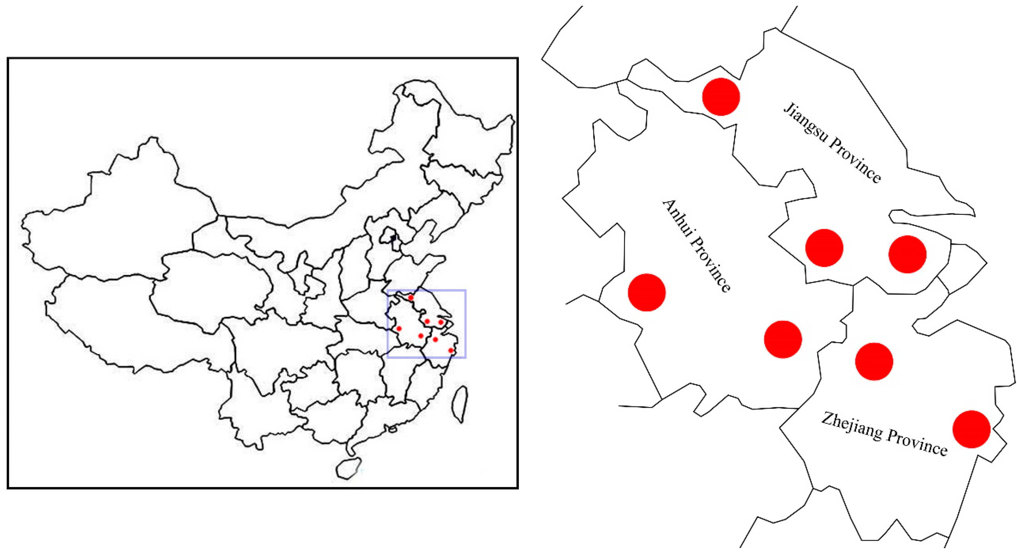
To date, reports regarding the genetic diversity and adaptive mechanisms in Chinese elms remain remarkably scant. In this study, we attempt to explore the genetic diversity of seven natural populations of Chinese elms in eastern China, and then identify the potential local adaptation genes based on SLAF-seq identified SNPs. Our results might help in the marker-assisted breeding of Chinese elms in the future.

2. Materials and Methods

2.1. Plant Materials

Natural populations of Ulmus parvifolia were investigated in the present study. A total of seven populations with 107 individuals were collected from Jiangsu Province (XZ, JN, CS), Anhui Province (HUOS, HS), and Zhejiang Province (FY, LH). For each population, 13~17 individuals were sampled, with individuals at least 300 m apart. Collection details and climate information for the seven populations are summarized in

Table 1. Population details of Chinese elms and their climate information.

Population Location	Abbreviation	Sample Size	Annual Rainfall (cm)	Geographical Coordinates	Annual Average Temperature (°C)	Altitude (m)
Xuzhou, Jiangsu	XZ	15	802.5	34°12′ N, 117°09′ E	14.5 (0.7, 27.3) *	56
Jiangning, Jiangsu	JN	13	1072.9	31°51′ N, 118°46′ E	15.7 (2.9, 28.3)	20
Changsu, Jiangsu	CS	17	1615.3	31°39′ N, 120°39′ E	16.9 (3.6, 28.2)	90
Huoshan, Anhui	HUOS	15	1366	31°26′ N, 116°23′ E	15.3 (2.6, 27.7)	110
Huangshan, Anhui	HS	14	2395	30°15′ N, 118°08′ E	15.5 (4.4, 28.1)	180
Fuyang, Zhejiang	FY	16	1441.9	30°03′ N, 119°37′ E	16.1 (4.3, 28.8)	90
Linhai, Zhejiang	LH	17	1550	28°47′ N, 121°34′ E	17.1 (6.5, 28.6)	10

* The values in brackets represent the average temperature over years in January and July.

and Figure 1 Young healthy leaves were sampled and stored at −80 °C until further use.

2.2. High-Throughput Sequencing

About 20 mg of leaves were used for genomic DNA extraction via the DNeasy Plant Pro Kit (Qiagen, Hilden, Germany). DNA concentration and quality were assessed with a Nanodrop 1000 Spectrophotometer (Thermo Fisher Scientific, Wilmington, MA, USA) and 2% agarose gel electrophoresis. Quantified DNA samples were diluted to 100 ng/µL for the subsequent SLAF-seq analysis. SLAF-seq was performed according to a previous report [12], with some modifications. Since the genome of Chinese elm has not been published, we used the Trema orientale (the same species in Ulmaceae) for the prediction of enzyme digestion. Briefly, the reference genome of Trema orientale was used to perform marker discovery surveys through simulating in silico the number of markers obtained by various restriction enzymes. To get >100,000 SLAF tags that were evenly distributed in the genome, two restriction enzymes, HinCII and HaeIII, were finally selected. The efficiency of enzyme digestion was of importance for the reduced-representation sequencing. For the present study, Oryza sativum ssp. japonica DNA with a high-quality genomic information was used as a control to evaluate the quality of enzyme digestion. Following digestion, a single nucleotide (A) was added to the 3′ end using dATP at 37 °C, and then Dual-index adapters were ligated to the A-tailed DNA fragments. PCR amplification was subsequently performed using diluted restriction-ligation DNA as the template. The products of PCR were purified and pooled together. DNA fragments that were 414–464 in length were collected from agarose gel, and were chosen as SLAF tags. High-throughput sequencing was performed using an Illumina-HiSeq^TM 2500 sequencing platform (Illumina, Inc.; San Diago, CA, USA) at Beijing Biomarker Technologies Corporation (Beijing, China).

2.3. SNP Calling

Raw reads generated from the sequencing platform were first qualified through removing the adapter sequence included in the raw reads, low-quality reads (quality scores < 20), and empty reads (reads just contained adapter sequence). High quality paired-end reads were clustered using the BLAT software based on sequence similarity [16]. Sequences with over 90% similarity among different individuals were identified as one SLAF locus [12]. Samtools [17] and the Genome Analysis Toolkit (GATK) [18] were used for SNP calling, and their intersection was considered to indicate reliable SNPs. For the phylogenetic analysis, SNPs with a minor allele frequency (MAF) < 5% and missing rate > 0.2 were filtered.

2.4. Diversity Analysis

A total of 457,888 SNPs from 107 individuals were developed to calculate the genetic diversity and population structure. The commonly used indexes of genetic diversity, including the observed allele number (Na), expected allele number (Ne), observed heterozygous number (Ho), expected heterozygous number (He), Nei’s diversity index (H), Shannon’s wiener index (I), and polymorphism information content (PIC), were calculated by POPGENE [19]. These indexes were calculated to estimate the degree of allele distribution (Na and Ne), genomic heterozygosity (Ho and He), gene diversity (H and I) and DNA polymorphism (PIC). In order to assess the population differentiation, Analysis of molecular variance (AMOVA) was calculated to estimate the partitioning of genetic variance among populations. Meanwhile, pairwise fixation index (Fst) among populations was also computed to detect how gene diversity was partitioned at each level. Inter-individual fixation index (FIS) was analyzed to determine the deviation of genotype frequencies from Hardy–Weinberg proportions within each population. AMOVA, Fst, and FIS were estimated by Arlequin [20].

The phylogenetic tree was constructed by MEGA X software with the following parameters: neighbor-joining method, Kimura 2-parameter model, and 1000 bootstrap replicates. The population structure was analyzed by Admixture [21], on the basis of the maximum-likelihood method. The number of populations (K), ranging from 1 to 10, was tested, and each individual was assigned to its respective populations according to the maximum membership probability.

2.5. Climatic Association Analysis

Two programs, Bayenv2 [22,23] and LFMM [24], were used to detect outlier loci that were possibly associated with climatic variables. First, we used Bayenv2 to detect correlations between SNP allele frequencies and environmental variables. A covariance matrix of allele frequencies was estimated across populations using the full set of SNPs to avoid population-specific effects. For each tested SNP, this program generated a Bayes factor (BF) and nonparametric Spearman’s rank correlation coefficient (ρ) based on the Markov chain Monte Carlo (MCMC). In this study, the significance threshold for the putative adaptive makers were those ranked among the top 1% of BF values (log₁₀BF > 2.75) and top 5% of ρ values. The other software, LFMM, was also used for gene-climate association analysis. As it estimates the hidden impact of population structure, LFMM permits the presence of background levels of population structure (latent factors). The detected SNPs that exhibit an association with the environment were determined according to the z-score. Bonferroni adjustment was used on the z-score values for multiple tests. Markers with z-scores > 2.8 and a p-value < 0.01 were considered to be significant. Putative functions for the identified outlier loci were annotated using the NCBI and UniProt databases.

3. Results

3.1. SNP Detection

High-throughput sequencing based on SLAF generated a total of 439.74 M pair-end reads, with a mean GC content of 42.90%, and an average Q30 of 96.70%. We obtained a total of 2,059,418 high-quality SLAF tags for the 107 samples, with an average depth of 18.88x for each SLAF (

Table 2. Summary of specific locus amplified fragment sequencing (SLAF-seq).

	No. of Reads	GC Content (%)	Q30 (%)	No. of SLAF	No. of Depth
Sum	439,742,148			2,059,418
Avg.	4,109,739.70	42.9	96.7	19,246.90	18.88

). For the SLAF tags, 529,271 were polymorphic. These polymorphic SLAFs contained 4,138,972 SNPs in total, and 457,888 of them were utilized in further analysis after applying the filtering criteria.

3.2. Genetic Diversity and Genetic Differentiation

The value of the observed allele number (Na) was 2 across populations, and the values of the expected allele number (Ne) ranged from 1.5321 (XZ) to 1.5759 (FY), with a mean value of 1.5498. The observed heterozygous (Ho) values were significantly lower than the He values, with values lying between 0.1483 (CS) and 0.1822 (FY), and an average of 0.1599. The values of the expected heterozygous (He) number across the seven populations were between 0.3236 (XZ) and 0.3427 (FY), with an average value of 0.3315. Nei’s diversity index (H) was within the range from 0.3385 (XZ) to 0.3570 (FY), with a mean value of 0.3467. Shannon’s wiener index (I) varied from 0.4948 to 0.5171 for the XZ and FY populations, respectively. The PIC values of the seven populations ranged from 0.2632 to 0.2761, with an average of 0.2686. The maximum value of PIC was presented in the FY population, while the minimum value was found in the XZ population. As a measure of intragametophytic selfing, F_IS were low in our study, varying from −0.03849 (FY population) to 0.06769 (HS population) (

Table 3. Genetic diversity of seven Chinese elm populations.

Population	Na	Ne	Ho	He	H	I	PIC	FIS
XZ	2	1.5321	0.1582	0.3236	0.3385	0.4948	0.2632	0.04448
JN	2	1.5462	0.1572	0.3298	0.3476	0.5021	0.2675	0.05903
CS	2	1.5362	0.1483	0.3255	0.3390	0.4971	0.2645	0.05467
HUOS	2	1.5414	0.1510	0.3281	0.3435	0.5002	0.2664	0.06443
HS	2	1.5469	0.1523	0.3307	0.3475	0.5034	0.2682	0.06769
FY	2	1.5759	0.1822	0.3427	0.3570	0.5171	0.2761	−0.03849
LH	2	1.5697	0.1699	0.3398	0.3534	0.5137	0.2741	0.01339

Na, observed allele number; Ne, expected allele number; Ho, observed heterozygous; He, expected heterozygous; H, Nei’s diversity index; I, Shannon’s wiener index; PIC, polymorphism information content; F_IS, inter-individual fixation index.

). All the F_IS were on Hardy–Weinberg equilibrium (p > 0.05).

The pairwise fixation index (Fst) is a measure of genetic differentiation among populations. In our study, the lowest genetic differentiation existed between the HS and HUOS populations, with an Fst value of 0.00712. The LH and XZ populations presented the largest genetic differentiation, with an Fst value of 0.09106 (

Table 4. Pairwise fixation index (Fst) values among seven populations of Chinese elm.

	XZ	JN	CS	HUOS	HS	FY
JN	0.03396
CS	0.03939	0.01504
HUOS	0.02869	0.01164	0.01525
HS	0.04646	0.01845	0.017	0.00712
FY	0.08368	0.05256	0.04706	0.04659	0.04891
LH	0.09106	0.0536	0.04831	0.05281	0.05296	0.07493

). AMOVA indicated that the maximum diversity occurred within individuals (92.22%), while the minimum diversity presented among individuals within populations (3.54%). A total of 4.24% of the genetic variation occurred among populations (

Table 5. Analysis of molecular variance (AMOVA) of genetic diversity of Chinese elm populations.

Source of Variation	df	Sum of Squares	Variance Components	Percentage of Variation (%)
Among populations	6	30,354.88	93.79375	4.24
Among individuals within populations	100	219,566.2	78.17923	3.54
Within individuals	107	218,205.5	2039.304	92.22

).

3.3. Phylogenetic Relationship and Population Structure

The genetic relationships of the 107 individuals were exemplified by a phylogenetic tree. Interestingly, we found that the individuals could not be divided into distinct clades, which indicates a weak population structure of the individuals (Figure 2). Generally, individuals in the same subclade were from the same population (Figure 2).

The genetic structure of the U. parvifolia populations was assessed with the Admixture software. As shown in Figure 3, the lowest K-values were detected when K = 1, indicating that a weak population structure existed in the individuals. A relatively low K-values was seen when K = 2, and correspondingly, the 107 individuals could be categorized into two groups. Group I contained 91 individuals, which were mainly from the FY, MH, HS, XZ, JN, and CS populations. Group II consisted only of 16 individuals from the LH population (Figure 4). Individuals with a low degree of admixture were seen from all the studied populations.

3.4. Association between SNP Markers and Environmental Variables

The association analysis of SNPs and environmental variables was conducted by the Bayenv2 and LFMM programs. Bayenv2 analysis identified a total of 43 SNP markers showing significant correlation with the environmental variables. Of these, 8, 10, and 25 markers were associated with altitude, annual rainfall, and annual average temperature, respectively (

Table 6. A summary of putative adaptive markers displaying associations with different climate variables identified by Bayenv2 analysis.

SNP ID	Pos	log10 (BF)	ρ	Altitude	Annual Rainfall	Annual Average Temperature
Marker127061	164	4.9954	0.1019	*
Marker58279	222	4.1913	0.1049	*
Marker204041	6	4.1152	0.1288	*
Marker971355	147	3.8946	0.1053	*
Marker62103	215	3.5162	0.1594	*
Marker76627	243	3.3182	0.1087	*
Marker54757	5	2.3134	0.1045	*
Marker33355	188	2.0794	0.1071	*
Marker129188	112	25.6440	0.1808		*
Marker39336	258	11.2230	0.1233		*
Marker201123	242	7.7245	0.1258		*
Marker44387	8	6.1236	0.1641		*
Marker40822	186	3.5858	0.1087		*
Marker68303	61	2.9905	0.1092		*
Marker85734	99	2.8768	0.1019		*
Marker71488	44	2.8301	0.1134		*
Marker37050	59	2.6988	0.1115		*
Marker58475	77	2.2600	0.1380		*
Marker41305	13	37.3380	0.1019			*
Marker62540	103	23.1980	0.1043			*
Marker107170	225	22.4260	0.1838			*
Marker65958	170	21.5660	0.1102			*
Marker18102	240	20.3570	0.1169			*
Marker18740	56	13.0760	0.1192			*
Marker60000	154	11.8650	0.1013			*
Marker78616	181	11.4110	0.1134			*
Marker29379	156	10.9290	0.1295			*
Marker112072	227	7.3602	0.1023			*
Marker62404	182	7.2272	0.1218			*
Marker116716	258	6.6439	0.1066			*
Marker211065	76	4.9942	0.1024			*
Marker145731	238	4.6537	0.1030			*
Marker2846306	228	4.0441	0.1947			*
Marker32405	256	3.6509	0.1019			*
Marker109530	179	3.5689	0.1013			*
Marker24830	245	3.4366	0.1058			*
Marker60529	214	3.4104	0.1613			*
Marker29189	49	3.0557	0.1021			*
Marker51336	148	2.8289	0.1259			*
Marker31333	33	2.4288	0.1735			*
Marker130465	24	2.3988	0.1026			*
Marker65370	245	2.3645	0.1109			*
Marker41605	187	2.0949	0.1111			*

* suggests that the SNP showed an association with that specific climate variable.

). A set of 30 markers associated with climatic variables was obtained by the LFMM program. The highest number of associations was for temperature, which was related to 16 markers; the annual rainfall and altitude were correlated with 4 and 10 markers, respectively (

Table 7. A summary of putative adaptive markers displaying associations with different climate variables identified by LFMM analysis.

SNP ID	Position	Z-Scores	log10(p)	p-Value	Altitude	Annual Rainfall	Annual Average Temperature
Marker45074	257	2.94	2.39	0.0041	*
Marker172745	21	2.90	2.34	0.0046	*
Marker45074	62	2.88	2.32	0.0048	*
Marker45074	10	2.87	2.30	0.0050	*
Marker45074	12	2.86	2.29	0.0051	*
Marker45074	69	2.86	2.29	0.0051	*
Marker45074	77	2.85	2.28	0.0052	*
Marker45074	253	2.85	2.28	0.0053	*
Marker45074	197	2.85	2.27	0.0053	*
Marker141529	57	−2.82	2.24	0.0057	*
Marker101622	111	2.93	2.38	0.0042		*
Marker101622	23	2.92	2.37	0.0043		*
Marker101622	75	2.92	2.37	0.0043		*
Marker101622	74	2.80	2.22	0.0061		*
Marker147012	258	−2.95	2.40	0.0040			*
Marker147012	172	2.94	2.40	0.0040			*
Marker147012	147	2.94	2.40	0.0040			*
Marker147012	59	−2.94	2.40	0.0040			*
Marker79339	199	2.94	2.40	0.0040			*
Marker112495	159	−2.94	2.40	0.0040			*
Marker112495	155	2.94	2.40	0.0040			*
Marker79339	63	2.94	2.40	0.0040			*
Marker87380	208	2.94	2.40	0.0040			*
Marker102725	233	−2.94	2.39	0.0040			*
Marker43598	85	2.94	2.39	0.0040			*
Marker58232	213	2.94	2.39	0.0041			*
Marker106952	19	−2.94	2.39	0.0041			*
Marker112495	237	−2.94	2.39	0.0041			*
Marker106952	94	−2.94	2.39	0.0041			*
Marker112495	238	−2.94	2.39	0.0041			*

* suggests that the SNP showed an association with that specific climate variable.

). Blast searches indicated that five of the correlated SNP markers could be annotated. Two markers (Marker204041 and Marker76627) associated with altitude could be annotated to the DEAD-box helicase and V-type proton ATPase genes, respectively. The SNP markers, Marker68303 and Marker129188, correlated with annual rainfall, were found in the regions of the UDP-glycosyltransferase (UGT) and peroxisome biogenesis protein genes, respectively. The SNP marker, Marker87380, associated with annual average temperature, seems to underlie the Cysteine-rich receptor-like protein kinase gene (

Table 8. Identification of putative candidate genes of the associated SNP markers.

Climate Variables	Marker ID	Position	Putative Genes
Altitude	Marker204041	6	DEAD-box helicase
	Marker76627	243	V-type proton ATPase
Annual rainfall	Marker68303	61	UDP-glycosyltransferase
	Marker129188	112	Peroxisome biogenesis protein
Annual average temperature	Marker87380	208	Cysteine-rich receptor-like protein kinase

).

4. Discussion

The present study is the first attempt to use SNPs derived from SLAF to assess the genetic diversity and explore the adaptation mechanisms of Chinese elms. In recent years, SLAF-seq technology has become a low-cost technique to effectively develop reliable SNP and InDel markers for genome-wide association analysis and high-density genetic map construction [25,26]. Our study identified a total of 4,138,972 SNPs and selected 457,888 SNPs with MAF > 5% and a missing rate < 0.2 for further analysis. The number of molecular markers was dramatically larger than that in previous reports on elm species [27,28], which facilitates precise genetic analysis.

Heterozygosity is an important measure of overall genetic diversity [25]. In our study, the Ho and He values ranged from 0.1483 to 0.1822 (an average of 0.1599) and 0.3236 to 0.3427 (an average of 0.3315), respectively (Table 3). These values were lower than the results observed in other trees [25,29]. A relative lower level of genetic heterozygosity for the Chinese elms might be due to the existence of spatial isolation in different groups, hindering the gene communication between individuals to some extent. The index, PIC, measures the degree of informativeness of a genetic marker, with values ranging from 0 to 1 [29]. A locus with a PIC value of 0 is undesirable [30]. When PIC < 0.25, it indicates a low polymorphism, and 0.25 < PIC < 0.50 represents a median polymorphism. In contrast, PIC > 0.50 is indicative of high polymorphism [31]. According to this criteria, as the PIC values were between 0.2632 to 0.2761 (Table 3), the tested seven populations in our study possessed medium genetic diversity in terms of PIC. The inter-individual fixation index (FIS) measures the deviation of genotype frequencies from Hardy–Weinberg proportions within each population. A negative FIS indicates heterozygote excess (outbreeding), while a positive value reflects a deficiency in heterozygosity (inbreeding) [32]. In our study, the FY population presented a negative FIS (−0.03849) (Table 3), suggesting a slight excess of heterozygotes. The other six populations exhibited a positive FIS (Table 3). All the populations were not statistically significantly deviated from the Hardy–Weinberg equilibrium (p > 0.05), indicating a relatively random mating for these populations. Overall, the FY population displayed higher genetic diversity than the other six populations, which was supported by the larger Ne, Ho, He, H, I, and PIC values (Table 3).

Outcrossing woody plants tend to possess low levels of genetic differentiation among populations [33]. In the current study, differentiation among populations was estimated by Fst values. Fst > 0.25 signifies a great genetic differentiation, 0.25 > Fst > 0.15 indicates a moderate genetic differentiation, 0.15 > Fst > 0.05 means a small genetic differentiation, and Fst < 0.05 represents negligible genetic differentiation [34]. Based on this standard, a low genetic differentiation was found among the studied populations (Fst values ranging from 0.00712 to 0.09106) (Table 4). Additionally, AMOVA analysis (Table 5) also indicated a low percentage of variation (4.24%) among populations. Similar results could be found in other trees [7,35].

Investigating the population structure of tested individuals is the premise for association analysis, since the presence of the population structure could affect the validity of association results [36,37,38]. In our study, the optimal K value of the seven populations was 1 (Figure 2), indicating no population structure existed in the studied groups. The geographic boundaries had a weak effect on the genetic structure of Chinese elms. The existence of population structure might cause correlations between unlinked locis, and would usually result in increased false associations, the weak population structure of Chinese elm in our study would be conducive to subsequent association analysis.

Natural selection has an important impact on shaping the genetic variation of a population, and therefore promotes local adaptation [39]. In this research, based on the identified SNP markers, an association study was used to uncover the hidden genetic basis of local adaptation. The associated SNP markers were blasted against public databases for putative genes. We found that the genes of DEAD-box helicase and V-type proton ATPase seemed to be candidates for adaptation to altitude. DEAD-box helicase is involved in nucleic acid metabolism functions, such as transcription, translation, replication, repair, recombination, ribosome biogenesis and splicing, which control plant grow and development [40]. V-type ATPase, as a transporter, is essential for energy metabolism and maintenance of solute homeostasis, which makes it indispensable for plant growth [41,42]. V-type proton ATPase has been shown to play a significant role in plant adaptation to stressful growth conditions [42]. We deduced that variations in altitude would lead to a difference in plant growth according to the functions of DEAD-box helicase and V-type proton ATPase.

UDP-glycosyltransferase (UGT) and peroxisome biogenesis protein were associated with annual rainfall variable. UGT belongs to the glycosyltransferase (GT) multigene family [43]. In plants, GTs are a ubiquitous group of enzymes involved in the glycosylation process, and glycosylation leads to the formation of glycosylated secondary chemicals such as flavonols, anthocyanins, and plant hormones [44,45]. Glycosylated secondary products possess increased water solubility and molecule stability, which could change their biological activity [44]. Peroxisome biogenesis protein might participate in the synthesis of peroxisomes, a metabolic organelle that exists in all eukaryotic cells [46]. Peroxisomes contribute to resistance against oxidative stresses, β- and α-oxidation of fatty acids, and synthesis of ether lipids [47,48]. The products of UGT and Peroxisome biogenesis protein seemed to confer advantages for plants survival in rainy climate [43]. It is reasonable that UGT and peroxisome biogenesis protein appeared as candidates for adaptation to rainfall climate.

Cysteine-rich receptor-like protein kinase (CRK) was the putative gene that we found was associated with the annual average temperature variable. CRKs are critical signaling components that regulate plant developmental and defense processes. In Arabidopsis, overexpression of a CRK gene confers drought tolerance without affecting plant growth [49]. Considering that the temperature variable would be generally correlated with drought stress, it is possible that there may be a difference in drought-associated loci among populations. Identification of putative candidate genes correlated with the environment would reveal a primary insight into functional genes mediating local adaptation. However, further studies are required in the future to explain the accurate roles of those candidate genes in the adaptation processes of Chinese elms.

5. Conclusions

The present study analyzed the genetic diversity and adaptation of seven natural populations of Chinese elms in eastern China. The trees were genotyped by SLAF-seq technology, and then identification of SNPs was carried out. The natural population of Chinese elms showed a moderate level of genetic diversity (PIC = 0.2632~0.2761), low level of genetic differentiation, and a simple population structure (K = 1). The association analysis of genetic markers and environmental factors resulted in putative markers involved in local adaptation. A blast search was conducted to detect underlying putative candidate genes for the correlated markers. A total of five genes could be annotated, which were related to the functions of glycosylation, peroxisome synthesis, nucleic acid metabolism, energy metabolism, and signaling. The results will be helpful for future work on molecular breeding of this species.

References

1. Thakur, R.; Karnosky, D. Micropropagation and germplasm conservation of Central Park Splendor Chinese elm (Ulmus parvifolia Jacq. ‘A/Ross Central Park’) trees. Plant Cell Rep. 2007, 26, 1171–1177. [Google Scholar] [CrossRef]
2. Wei, X.; Xizeng, X.; Shouqian, Z. Variation of physiological and biochemical Iindexes in seedlings of three Ulmaceae species under water stress. J. Nanjing For. Univ. 2005, 29, 47–50. [Google Scholar]
3. Zhang, Q.; Li, C.; Yang, Q.; Zhou, J.; Zhang, D. Efforts of drought resistance characteristics and mechanism of the compensation in Ulmus parvifolia Jacq seedlings. Shandong For. Sci. Technol. 2017, 5, 22–26. [Google Scholar]
4. Yu, Y.; Wang, C.; Wang, H.; Li, C.; Sun, Z. Comparison of drought tolerance, salt tolerance and moisture tolerance in varieties of trees. J. Agric. 2015, 5, 113–116. [Google Scholar]
5. Aitken, S.N.; Yeaman, S.; Holliday, J.A.; Wang, T.; Curtis-McLane, S. Adaptation, migration or extirpation: Climate change outcomes for tree populations. Evol. Appl. 2008, 1, 95–111. [Google Scholar] [CrossRef] [PubMed]
6. Eding, H.; Crooijmans, R.P.; Groenen, M.A.; Meuwissen, T.H. Assessing the contribution of breeds to genetic diversity in conservation schemes. Genet. Sel. Evol. 2002, 34, 613. [Google Scholar] [CrossRef] [Green Version]
7. Yang, Z.; Wang, L.; Zhao, T. High genetic variability and complex population structure of the native Chinese hazelnut. Braz. J. Bot. 2018, 41, 687–697. [Google Scholar] [CrossRef]
8. Abebe, T.D.; Naz, A.A.; Léon, J. Landscape genomics reveal signatures of local adaptation in barley (Hordeum vulgare L.). Front. Plant Sci. 2015, 6, 813. [Google Scholar] [CrossRef] [PubMed] [Green Version]
9. Vangestel, C.; Vázquez-Lobo, A.; Martínez-García, P.J.; Calic, I.; Wegrzyn, J.L.; Neale, D.B. Patterns of neutral and adaptive genetic diversity across the natural range of sugar pine (Pinus lambertiana Dougl). Tree Genet. Genomes 2016, 12, 51. [Google Scholar] [CrossRef]
10. Tsumura, Y.; Uchiyama, K.; Moriguchi, Y.; Ueno, S.; Ihara-Ujino, T. Genome scanning for detecting adaptive genes along environmental gradients in the Japanese conifer, Cryptomeria japonica. Heredity 2012, 109, 349. [Google Scholar] [CrossRef] [PubMed] [Green Version]
11. Brookes, A.J. The essence of SNPs. Gene 1999, 234, 177–186. [Google Scholar] [CrossRef]
12. Sun, X.; Liu, D.; Zhang, X.; Li, W.; Liu, H.; Hong, W.; Jiang, C.; Guan, N.; Ma, C.; Zeng, H. SLAF-seq: An efficient method of large-scale de novo SNP discovery and genotyping using high-throughput sequencing. PLoS ONE 2013, 8, e58700. [Google Scholar] [CrossRef] [PubMed]
13. Elshire, R.J.; Glaubitz, J.C.; Sun, Q.; Poland, J.A.; Kawamoto, K.; Buckler, E.S.; Mitchell, S.E. A robust, simple genotyping-by-sequencing (GBS) approach for high diversity species. PLoS ONE 2011, 6, e19379. [Google Scholar] [CrossRef] [PubMed] [Green Version]
14. Bentley, N.; Grauke, L.; Klein, P. Genotyping by sequencing (GBS) and SNP marker analysis of diverse accessions of pecan (Carya illinoinensis). Tree Genet. Genomes 2019, 15, 8. [Google Scholar] [CrossRef]
15. Bai, Q.; Cai, Y.; He, B.; Liu, W.; Pan, Q.; Zhang, Q. Core set construction and association analysis of Pinus massoniana from Guangdong province in southern China using SLAF-seq. Sci. Rep. 2019, 9, 1–13. [Google Scholar] [CrossRef]
16. Kent, W.J. BLAT—The BLAST-like alignment tool. Genome Res. 2002, 12, 656–664. [Google Scholar] [CrossRef] [Green Version]
17. Li, H.; Handsaker, B.; Wysoker, A.; Fennell, T.; Ruan, J.; Homer, N.; Marth, G.; Abecasis, G.; Durbin, R. The sequence alignment/map format and SAMtools. Bioinformatics 2009, 25, 2078–2079. [Google Scholar] [CrossRef] [Green Version]
18. McKenna, A.; Hanna, M.; Banks, E.; Sivachenko, A.; Cibulskis, K.; Kernytsky, A.; Garimella, K.; Altshuler, D.; Gabriel, S.; Daly, M. The Genome Analysis Toolkit: A MapReduce framework for analyzing next-generation DNA sequencing data. Genome Res. 2010, 20, 1297–1303. [Google Scholar] [CrossRef] [Green Version]
19. Yeh, F.C.; Yang, R.-C.; Boyle, T. POPGENE version 1.31. In Microsoft Window-Based Freeware for Population Genetic Analysis; University of Alberta: Edmonton, AB, Canada, 1999. [Google Scholar]
20. Excoffier, L.; Laval, G.; Schneider, S. Arlequin (version 3.0): An integrated software package for population genetics data analysis. Evol. Bioinform. 2005, 1, 47–50. [Google Scholar] [CrossRef] [Green Version]
21. Alexander, D.H.; Novembre, J.; Lange, K. Fast model-based estimation of ancestry in unrelated individuals. Genome Res. 2009, 19, 1655–1664. [Google Scholar] [CrossRef] [PubMed] [Green Version]
22. Coop, G.; Witonsky, D.; Di Rienzo, A.; Pritchard, J.K. Using environmental correlations to identify loci underlying local adaptation. Genetics 2010, 185, 1411–1423. [Google Scholar] [CrossRef] [Green Version]
23. Günther, T.; Coop, G. Robust identification of local adaptation from allele frequencies. Genetics 2013, 195, 205–220. [Google Scholar] [CrossRef] [PubMed] [Green Version]
24. Frichot, E.; Schoville, S.D.; Bouchard, G.; François, O. Testing for associations between loci and environmental gradients using latent factor mixed models. Mol. Biol. Evol. 2013, 30, 1687–1699. [Google Scholar] [CrossRef] [PubMed] [Green Version]
25. Li, B.; Tian, L.; Zhang, J.; Huang, L.; Han, F.; Yan, S.; Wang, L.; Zheng, H.; Sun, J. Construction of a high-density genetic map based on large-scale markers developed by specific length amplified fragment sequencing (SLAF-seq) and its application to QTL analysis for isoflavone content in Glycine max. BMC Genom. 2014, 15, 1086. [Google Scholar] [CrossRef] [PubMed] [Green Version]
26. Luo, C.; Shu, B.; Yao, Q.; Wu, H.; Xu, W.; Wang, S. Construction of a High-Density Genetic Map Based on Large-Scale Marker Development in Mango Using Specific-Locus Amplified Fragment Sequencing (SLAF-seq). Front. Plant Sci. 2016, 7, 1310. [Google Scholar] [CrossRef] [PubMed] [Green Version]
27. Lee, I.M.; Davis, R.E.; Sinclair, W.A.; Dewitt, N.D.; Conti, M. Genetic relatedness of mycoplasmalike organisms detected in Ulmus spp. in the United States and Italy by means of DNA probes and polymerase chain reactions. Phytopathology 1993, 83, 829–833. [Google Scholar] [CrossRef]
28. Pooler, M.R.; Townsend, A.M. DNA fingerprinting of clones and hybrids of American elm and other elm species with AFLP markers. J. Environ. Hortic. 2005, 23, 113–117. [Google Scholar]
29. Tahan, O.; Geng, Y.; Zeng, L.; Dong, S.; Chen, F.; Chen, J.; Song, Z.; Zhong, Y. Assessment of genetic diversity and population structure of Chinese wild almond, Amygdalus nana, using EST-and genomic SSRs. Biochem. Syst. Ecol. 2009, 37, 146–153. [Google Scholar] [CrossRef]
30. Ince, A.; Elmasulu, S.; Cinar, A.; Karaca, M.; Onus, A.; Turgut, K. Comparison of DNA marker techniques for Lamiaceae. In Proceedings of the I International Medicinal and Aromatic Plants Conference on Culinary Herbs 826, Antalya, Turkey, 29 April–4 May 2007; pp. 431–438. [Google Scholar]
31. Botstein, D.; White, R.L.; Skolnick, M.; Davis, R.W. Construction of a genetic linkage map in man using restriction fragment length polymorphisms. Am. J. Hum. Genet. 1980, 32, 314. [Google Scholar]
32. Gultyaeva, E.; Aristova, M.; Shaidayuk, E.; Mironenko, N.; Kazartsev, I.; Akhmetova, A.; Kosman, E. Genetic differentiation of Puccinia triticina Erikss. in Russia. Russ. J. Genet. 2017, 53, 998–1005. [Google Scholar] [CrossRef]
33. Hamrick, J.L.; Godt, M.W. Effects of life history traits on genetic diversity in plant species. Philos. Trans. R. Soc. Lond. Ser. B Biol. Sci. 1996, 351, 1291–1298. [Google Scholar]
34. Sukonthabhirom, S.; Saengtharatip, S.; Jirakanchanakit, N.; Rongnoparut, P.; Yoksan, S.; Daorai, A.; Chareonviriyaphap, T. Genetic structure among Thai populations of Aedes aegypti mosquitoes. J. Vector Ecol. 2009, 34, 43–49. [Google Scholar] [CrossRef] [PubMed]
35. Zeinalabedini, M.; Dezhampour, J.; Majidian, P.; Khakzad, M.; Zanjani, B.M.; Soleimani, A.; Farsi, M. Molecular variability and genetic relationship and structure of Iranian Prunus rootstocks revealed by SSR and AFLP markers. Sci. Hortic. 2014, 172, 258–264. [Google Scholar] [CrossRef]
36. Arthur, K.; Vilhjálmsson, B.J.; Vincent, S.; Alexander, P.; Quan, L.; Magnus, N. A mixed-model approach for genome-wide association studies of correlated traits in structured populations. Nat. Genet. 2012, 44, 1066–1071. [Google Scholar]
37. Korte, A.; Farlow, A. The advantages and limitations of trait analysis with GWAS: A review. Plant Methods 2013, 9, 29. [Google Scholar] [CrossRef] [PubMed] [Green Version]
38. Gupta, P.K.; Rustgi, S.; Kulwal, P.L. Linkage disequilibrium and association studies in higher plants: Present status and future prospects. Plant Mol. Biol. 2005, 57, 461–485. [Google Scholar] [CrossRef]
39. Kawecki, T.J.; Ebert, D. Conceptual issues in local adaptation. Ecol. Lett. 2004, 7, 1225–1241. [Google Scholar] [CrossRef] [Green Version]
40. Tuteja, N.; Tarique, M.; Banu, M.S.A.; Ahmad, M.; Tuteja, R. Pisum sativum p68 DEAD-box protein is ATP-dependent RNA helicase and unique bipolar DNA helicase. Plant Mol. Biol. 2014, 85, 639–651. [Google Scholar] [CrossRef]
41. Boekema, E.; Ubbink-Kok, T.; Lolkema, J.; Brisson, A.; Konings, W. Visualization of a peripheral stalk in V-type ATPase: Evidence for the stator structure essential to rotational catalysis. Proc. Natl. Acad. Sci. USA 1997, 94, 14291–14293. [Google Scholar] [CrossRef] [Green Version]
42. Dietz, K.-J.; Tavakoli, N.; Kluge, C.; Mimura, T.; Sharma, S.; Harris, G.; Chardonnens, A.; Golldack, D. Significance of the V-type ATPase for the adaptation to stressful growth conditions and its regulation on the molecular and biochemical level. J. Exp. Bot. 2001, 52, 1969–1980. [Google Scholar] [CrossRef] [Green Version]
43. Mackenzie, P.I.; Owens, I.S.; Burchell, B.; Bock, K.W.; Bairoch, A.; Belanger, A.; Fournel-Gigleux, S.; Green, M.; Hum, D.W.; Iyanagi, T. The UDP glycosyltransferase gene superfamily: Recommended nomenclature update based on evolutionary divergence. Pharmacogenetics 1997, 7, 255–269. [Google Scholar] [CrossRef]
44. Caputi, L.; Malnoy, M.; Goremykin, V.; Nikiforova, S.; Martens, S. A genome-wide phylogenetic reconstruction of family 1 UDP-glycosyltransferases revealed the expansion of the family during the adaptation of plants to life on land. Plant J. 2012, 69, 1030–1042. [Google Scholar] [CrossRef]
45. Woo, H.-H.; Orbach, M.J.; Hirsch, A.M.; Hawes, M.C. Meristem-localized inducible expression of a UDP-glycosyltransferase gene is essential for growth and development in pea and alfalfa. Plant Cell 1999, 11, 2303–2315. [Google Scholar] [CrossRef] [Green Version]
46. De Duve, C.; Baudhuin, P. Peroxisomes (microbodies and related particles). Physiol. Rev. 1966, 46, 323–357. [Google Scholar] [CrossRef]
47. Brown, L.A.; Baker, A. Peroxisome biogenesis and the role of protein import. J. Cell. Mol. Med. 2003, 7, 388–400. [Google Scholar] [CrossRef] [PubMed] [Green Version]
48. Heiland, I.; Erdmann, R. Biogenesis of peroxisomes: Topogenesis of the peroxisomal membrane and matrix proteins. FEBS J. 2005, 272, 2362–2372. [Google Scholar] [CrossRef] [PubMed]
49. Lu, K.; Liang, S.; Wu, Z.; Bi, C.; Yu, Y.-T.; Wang, X.-F.; Zhang, D.-P. Overexpression of an Arabidopsis cysteine-rich receptor-like protein kinase, CRK5, enhances abscisic acid sensitivity and confers drought tolerance. J. Exp. Bot. 2016, 67, 5009–5027. [Google Scholar] [CrossRef] [PubMed] [Green Version]
Figure 1. Map showing locations of the populations of Chinese elm.
Forests 11 00080 g001
Figure 2. Phylogenetic tree of the 197 individuals based on the analysis of 457,888 single nucleotide polymorphisms (SNPs).
Forests 11 00080 g002
Figure 3. ADMIXTURE estimation of the number of groups for K values ranging from 1 to 10.
Forests 11 00080 g003
Figure 4. Population structure analysis of the 107 individuals based on 457,888 SNPs. The bars in the x-axis indicate different individuals. Colors in each row represent structural components.
Forests 11 00080 g004