Modeling of Aboveground Biomass with Landsat 8 OLI and Machine Learning in Temperate Forests

Abstract

An accurate estimation of forests’ aboveground biomass (AGB) is required because of its relevance to the carbon cycle, and because of its economic and ecological importance. The selection of appropriate variables from satellite information and physical variables is important for precise AGB prediction mapping. Because of the complex relationships for AGB prediction, non-parametric machine-learning techniques represent potentially useful techniques for AGB estimation, but their use and comparison in forest remote-sensing applications is still relatively limited. The objective of the present study was to evaluate the performance of automatic learning techniques, support vector regression (SVR) and random forest (RF), to predict the observed AGB (from 318 permanent sampling plots) from the Landsat 8 Landsat 8 Operational Land Imager (OLI) sensor, spectral indexes, texture indexes and physical variables the Sierra Madre Occidental in Mexico. The result showed that the best SVR model explained 80% of the total variance (root mean square error (RMSE) = 8.20 Mg ha⁻¹). The variables that best predicted AGB, in order of importance, were the bands that belong to the region of red and near and middle infrared, and the average temperature. The results show that the SVR technique has a good potential for the estimation of the AGB and that the selection of the model hyperparameters has important implications for optimizing the goodness of fit.

1. Introduction

Forest ecosystems, which cover 30% of the land surface, play a key role in the global carbon cycle, by mitigating anthropogenic emissions [1]. A more accurate estimation of the regional to global distribution of forest aboveground biomass is required to provide the baseline of forest carbon stocks, and to quantify the anthropogenic emissions caused by deforestation and forest degradation [2,3]. In addition, the quantification of forest biomass has large economic implications for the supply of goods such as wood, timber, food, fiber and energy [4,5]. Forest biomass has also important ecological implications in ecosystem sustainability, including soil and water management [6]. Moreover, forest biomass and its change also influence other ecosystem services, such as biodiversity [7].

Traditionally, forest biomass has been assessed using field-based inventory plots and destructive biomass sampling to establish biomass stocks at the tree and plot level and extrapolate estimates to regions with similar characteristics to the plots evaluated [8,9]. Whereas this approach is valuable and can be precise at a local scale, it is also expensive and time consuming, and inherently limited in geographic representativeness [10,11]. The natural variation in forest structure and biomass, combined with the enormous geographic extent and rate of forest loss and disturbance, makes field plots difficult to use (alone) for assessing forest biomass and carbon densities [12], particularly over large areas [13,14,15] such as Mexican forests [16]. The use of remote-sensing techniques, calibrated and validated with representative field sites of forest biomass monitoring, allows spatially representative maps of forest ecosystems’ structure and productivity to be derived, over larger areas, and at lower costs [17,18].

In particular, the availability of a large archive of free available medium-resolution satellite imagery, such as Landsat, has allowed their increased use in many applications, including the forests aboveground biomass (AGB) estimation at local and regional scales [19,20,21].

It is important to effectively employ suitable techniques to extract spectral variables for biomass estimation modeling [22]. The potential variables from Landsat Thematic Mapper (TM) images include individual spectral bands, vegetation indices, transformed images, textural images, and fractional images [23]. Although many vegetation indices have been proposed [24], depending on the complexity of forest stand structure, the spectral bands, vegetation indices and texture variables can vary in their relationships with biomass [22].

In addition, environmental conditions can have a large role in modulating spatial and temporal patterns of forest AGB [19,25,26]. Consequently, several studies have demonstrated the utility of considering climatic variables, such as temperature or precipitation, in improving the predictions of aboveground biomass from satellite images, particularly over large areas, where climate can largely influence forest species distribution, structure and growth [1,19,27].

Furthermore, topographic variables represent a local heterogeneous factor that influence on forest diversity, distribution and development, directly influencing forest productivity and structure [28]. The combination of spectral and topographic variables, such as elevation [12,29], slope and aspect [22,30], or topographic wetness indices [23] is, therefore, potentially useful for improving the mapping of forest productivity at a landscape scale.

Given the diversity of environmental, topographical and biophysical conditions in forest ecosystems in different locations, there is no universal, transferable technique for estimating biomass from remote sensors [6,19,31]. The best models to map biomass are reliant on the characteristics of the particular forest or landscape [32], resulting in a need to identify the most useful variables for biomass mapping at each area of study.

In addition to the selection of suitable spectral and environmental variables, the use of proper algorithms for establishing biomass estimation models is also critical [22]. Techniques for biomass estimation can be grouped into two broad categories: parametric and non-parametric algorithms [26]. Parametric algorithms assume that the relationships between dependent (i.e., biomass) and independent (spectral and environmental) variables have explicit model structures that can be specified a priori by parameters [22]. Examples are simple or multiple linear regression models [32,33]. Linear regression analysis is probably the most frequently used approach for predicting forest biomass and other forest attributes [34] as shown in the reviews by Mohd et al. [26], Brosofske et al. [32] and Zhang and Ni-Meister [33].

Frequently, the relationships between biomass and remote sensing variables are often too complex to be captured by parametric algorithms. Non-parametric algorithms do not explicitly predefine the model structure, and instead, determine the model structure in a data-driven manner [22]. One of the greatest advantages of non-parametric algorithms is that they are free from assumptions regarding the probability distribution and correlation of the input data [22,33]. Unlike both simple linear models and multiple regression models, this approach can handle a large number of variables from satellite and ancillary data and effectively solves complex non-linear relationships between the response and predictor variables [33]. As complex ecological systems like forests frequently show non-linear relationships, autocorrelation and variable interaction across temporal and spatial scales, non-parametric algorithms often outperform parametric ones [19,35].

The most utilized machine-learning non-parametric methods include nearest neighbor approaches (NN) [36,37], support vector machine (SVM) [38,39], among others. Whereas most of these techniques have shown improvements compared to parametric methods, one disadvantage of some of these methods (such as neuronal networks), is that they are black boxes algorithms that do not offer information of the model selected variables and structure [32]. In contrast, methods such as random forest or SVM allow an understanding and interpretation of the selected variables and the structure of the models developed [40,41,42].

SVM techniques [43] are increasingly being applied in remote sensing applications, including biomass prediction [44]. In SVM, the support vector regression (SVR) transforms the input data into a high-dimensional feature space using a nonlinear kernel function to minimize training error and the complexity of the model [45]. SVM employs the principle of structural risk minimization to simultaneously optimize performance and generalization to effectively alleviate the overfitting problem [46]. The method has shown a good intrinsic generalization ability and robustness to noise using limited training sample data to produce relatively higher classification or estimation accuracy than other approaches [22]. The key to this approach is identifying suitable parameters: the precision of an SVM model depends on the defined tolerance margin and on a cost function, which denotes the balance between the resulting model and the tolerated deviations [47]. In spite of the importance of model optimization for machine-learning techniques, studies that have considered parameter optimization for biomass prediction are relatively scarce.

Another non-parametric technique, RF, randomly selects independent data samples to establish relationship in an advanced hyperplane by constructing numerous small regression trees [41]. Only a small number of randomly selected predictor variables are used to find the best split at each node, decreasing the correlation between trees and reducing bias, which brings a higher stability to the final model [32,41,42]. This method can deal with large datasets with a large number of variables, it can readily accommodate nonlinear responses, variable interactions, both continuous and categorical explanatory variables, and is relatively unaffected by outliers or multicollinearity [22].

Studies comparing the performance of various machine-learning techniques are relatively scarce [19,44,48]. From these studies, we know there is little consensus on which statistical method or set of predictor variables is the most robust across a range of forest conditions [22]. Depending on the study, the best results have been obtained either with neuronal networks [49,50], RF [19,43,48] or SVM [48,51]. There is a need to better understand how the choice of model type affects predictions of biomass [19]. Furthermore, the selection of the best prediction technique might be site specific depending on the characteristics of the stands analyzed and the goals of the study [32].

The forests of the Sierra Madre Occidental (SMO), NW Mexico, provide a good opportunity to compare methodologies for predicting and mapping biomass from spectral, textural, topographic and climatic variables, because of their variation in complex and diverse forest structure and their diverse physiographic and climatic conditions [16,21,23,35]. Furthermore, the SMO is also important because of the presence of some of the most important commercial species of pine and oak in Mexican ecosystems [23]. In particular, the state of Durango generates between 25% and 30% of national timber production, producing a total of 1.5 million m³ of roundwood per year, and boasts forest reserves that are important sources of environmental services [16].

The current study aimed at evaluating the performance of machine-learning techniques RF and SVM to predict and map the observed AGB from 318 permanent sampling plots for the SMO forests in the state of Durango, from Landsat 8 Landsat 8 Operational Land Imager bands, vegetation indices, texture indices, topographic and climatic variables.

2. Materials and Methods

2.1. Study Area

The study area was located on the temperate forests of the Durango State on the western Sierra Madre, NW Mexico (Figure 1). These forests have rich biodiversity and include at least 27 coniferous tree species (of which 20 are Pinus species) and 43 species of Quercus; the predominant forest stands comprise pines and oaks, often mixed with Arbutus and Juniperus, among other tree species. The forest structure is irregular, both referring to the spatial arrangement of trees (vertical and horizontal irregularity) and to the variation in the age structure of trees and stands [52]. Elevation in the SMO ranges from 1364 to 3020 m above sea level. The annual average precipitation ranges between 443 and 1452 mm and the annual average temperature between 8 and 26 °C.

2.2. Field Data

A total of 318 permanent forest inventory plots were sampled during winter of 2017. Each permanent sampling plot, of 50 × 50 m, was established following the methodology described by Corral-Rivas et al. [53]. At every permanent forest inventory plot, Diameter at breast height (dbh) (cm) and total height (h) (m) was measured for every tree of >7 cm dbh. Tree volume was obtained from the equations of Corral et al. [54]. Aboveground biomass was estimated utilizing the species specific allometric models of Vargas-Larreta et al. [55]. The goodness of fit of those allometric models ranged from 0.87–0.99 (R²), and 22.8–95.2 kg (root mean square error, RMSE). The descriptive statistics of the main forest inventory variables of the sites of study are summarized in

Table 1. Descriptive statistics of the main forest inventory variables of the sites of study.

Variable	Mean	Standard Deviation	Minimum Value	Maximum Value
Number of trees per ha	164	74.48	34	566
Basal area (m2·ha−1)	5.61	2.10	0.84	14.45
Volume (m3·ha−1)	51.88	28.52	3.26	187.26
Aboveground biomass (Mg·ha−1)	28.83	16.76	1.72	101.71

. The plots covered a gradient from very open stands in the more arid areas in the Eastern part of the area of study to relatively denser stands in the colder and wetter Western part of the SMO.

2.3. Spectral Data from the Landsat 8 Operational Land Imager (OLI)

Spectral information from the satellite Landsat 8 (OLI) of the United States Geological Service (USGS), was retrieved for the forest area in the Durango State. A total of 7 scenes, with a low cloud percentage, were utilized (path/row: 30/44, 31/42, 31/43, 31/44, 32/41, 32/42 and 32/43). The satellite images corresponded to the months of April and May 2017. The wavelength and spectral resolution of the bands utilized are summarized in

Table 2. Characteristics of Landsat 8 Operational Land Imager bands.

Band	Name	Wavelength (μm)	Spatial Resolution (m)
BAND 02	Blue	0.45–0.51	30 × 30
BAND 03	Green	0.53–0.59	30 × 30
BAND 04	Red	0.64–0.67	30 × 30
BAND 05	Near Infrared (NIR)	0.85–0.88	30 × 30
BAND 06	Shortwave infrared (SWIR 1)	1.57–1.65	30 × 30
BAND 07	Shortwave infrared (SWIR 2)	2.11–2.29	30 × 30
BAND 09	Cirrus	1.36–1.38	30 × 30

.

A radiometric correction was performed to the images, with the goal of minimizing the effect of dispersion caused by the atmosphere on the radiances perceived by the satellite. The correction consists of converting the digital levels (DLs) to radiance values and then to apparent reflectance values. The word “apparent” refers to the fact that the reflectance has not been corrected for atmospheric effects and represents an initial normalization of the image [56]. The radiometric correction was carried out with the “apparent reflectance” method implemented in the “Landsat” package in the R software [57].

2.4. Vegetation Indices

After performing the radiometric correction, vegetation indices were generated as potential predictors for the AGB models, given their capacity of discriminating vegetation and soil. The normalized difference vegetation index (NDVI) and the soil-adjusted vegetation index (SAVI) were calculated following Equations (1) and (2). Both indices (widely utilized for prediction of forest biomass and other dasometric variables) utilize the maximum absorption of the red (R) and near infrared (NIR) wavelengths, which allow to evaluate the chlorophyll and leaf structure [58]. SAVI index includes also a correction factor for soil brightness to the near infrared band (L) [59].

$$\mathrm{NDVI}=\frac{\left(NIR-R\right)}{\left(NIR+R\right)}$$

(1)

$$\mathrm{SAVI}=\left[\frac{\left(NIR-R\right)}{\left(NIR+R+L\right)}\right]\left(1+L\right)$$

(2)

where:

• NIR: Near Infrared.
• R: Red.
• L: Is the soil brightness correction factor and its value is 0.5.

2.5. Texture Indices

The texture variable extraction was performed with the grey level co-occurrence matrix (GLCM), which is a method that has showed good results in the estimation of forest variables from spectral data [60]. The metrics of second order (co-occurrence) GLCM (

Table 3. Texture variables to estimate aboveground biomass (AGB).

Texture Variables	Formula
Mean	$ME={\displaystyle \sum _{i,j=1}^{N\mathrm{g}}}i\ast P\left(i,j\right)$
Standard deviation	$SD\sqrt{{\displaystyle \sum _{i,j=1}^{N_g}}{\left(i-u\right)}^2}P\left(i,j\right)$
Homogeneity	$HO={\displaystyle \sum _{i,j=0}^{N-1}}i\frac{P_{i,j}}{1+{\left(i-j\right)}^2}$
Contrast	$CO={\displaystyle \sum _{i,j=0}^{N-1}}i{P}_{i,j}{\left(i-j\right)}^2$
Dissimilarity	$DI={\displaystyle \sum _{i,j=0}^{N-1}}i{P}_{i,j}\left[i-j\right]$
Entropy	$EN={\displaystyle \sum _{i,j=0}^{N-1}}i{P}_{i,j}\left[-lni-P_{i,j}\right]$
Second moment	$SM={\displaystyle \sum _{i,j=0}^{N-1}}i{P}^2{}_{i,j}$
Correlation	$CC=\frac{{\displaystyle {\sum }_{i,j}}\left(ij\right)P\left(i,j\right)-{\mu }_x{\mu }_y}{{\sigma }_x{\sigma }_y}$

where: P (i,j): (i,j) the entry in a normalized gray-tone spatial-dependence matrix; Ng: Number of distinct gray levels in the quantized.

), associated to three different kernels (3 × 3, 5 × 5, 7 × 7), were calculated from NDVI with the software PCI Geomatics [61].

2.6. Topographic and Climatic Variables

The digital elevation model from INEGI (Instituto Nacional de Estadística y Geografía) [62], with a resolution of 15 m, was utilized.

A low pass filter in kernels of 5 × 5 was applied to remove the high frequency noise that would result in irregular artifacts in the topographic variables and indices [63,64].

Climatic variables were also considered because of their potential influence together with topography on the development and growth of forest biomass. The National Automated Agroclimatic Stations Network [65] was utilized as sources of climatic data. The climatic data were modeled utilizing kriging. Variables considered for analysis where those where the kriging modeling had fits with more than 90% statistical goodness of fit. The topographic and climatic variables considered for prediction of aboveground biomass are shown in

Table 4. Physical (topographic and climatic) variables and indices to predict aboveground biomass (AGB).

Physical Variable	Equation	Reference
Topographic
Slope	$s=arctan\left(\sqrt{p^2+q^2}\right)$	[66]
Elevation	$ELV=Z\left(x,y\right)$	[67]
Aspect	$\mathrm{T}\theta =arctan\left(\frac{-H}{-G}\right)$	[68]
Curvature	$C\chi =C\omega -C\varphi$	[69]
Plan curvature	$\mathrm{C}\omega =2\frac{D{H}^2+E{G}^2-FGH}{G^2+H^2}$
Profile curvature	$\mathrm{C}\varphi =-2\frac{D{G}^2+E{H}^2+FGH}{G^2+H^2}$
Wetness Index	$WI=\ln \left(A_s/\tan B\right)$	[70]
Heat load index	$HLI=\frac{1-cos\left(\theta -45\right)}{2}$	[71]
Aspect/Slope ratio	$G=b_o+B_{s}cos(a-\theta )+b_{3}s$	[72]
Climatic
Maximum Temperature (TM)	(°C)	[65]
Mean Annual Temperature (Tmed)	(°C)

where: p and q, are the components of the gradient vector of slope; Z, elevation; R, point radio altitude units; A_s, drainage area specified; tan B, local slope angle; D, F, G and H were derived according to the equation of [69]; $\theta$, Aspect in degrees east of north; G, growt response; $b_o$, constant term or sum of the predictor effects in the regression and B_s and b₃ are coefficients according to the equation of [72]; $a,$ azimuth in degress from north; $s,$ slope in percent/100.

.

2.7. Statistical Analysis

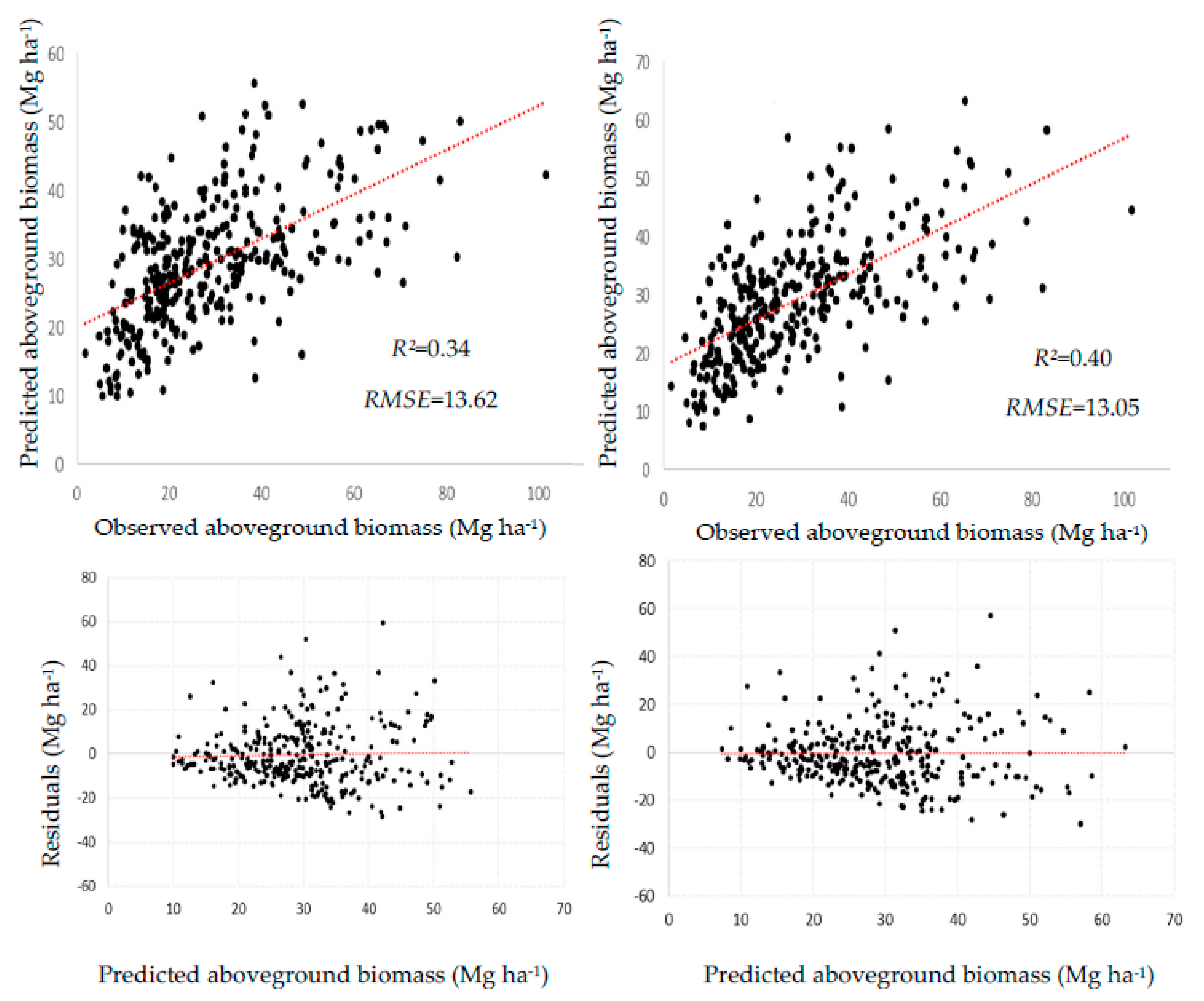
2.7.1. Support Vector Regression (SVR)

SVR is a machine-learning algorithm developed by Vapnik–Chervonenkis [44]. It is a robust machine-learning technique, mainly because of its high learning speed and the use of kernels that project data to a high-dimension new space termed the hyperplane [73]. The SVR regression model maps training data in a hyperplane regulated by a flexible boundary line that adjusts the prediction function. Under this principle it penalizes the vectors outside the margin of the boundary line (epsilon) [74].

The SVR model was implemented through the package e1071, in the statistical software R [75]. An initial evaluation was performed with a model with the default parameters from SVR. A sensitivity analysis of the cost and epsilon metaparameters was performed to optimize the model performance. A total of 88 models were evaluated in this optimization.

The independent variables considered to predict the inventory-derived AGB were the spectral bands (Table 2), the vegetation and texture indices (Table 3) and the topographic and environmental variables listed in Table 4.

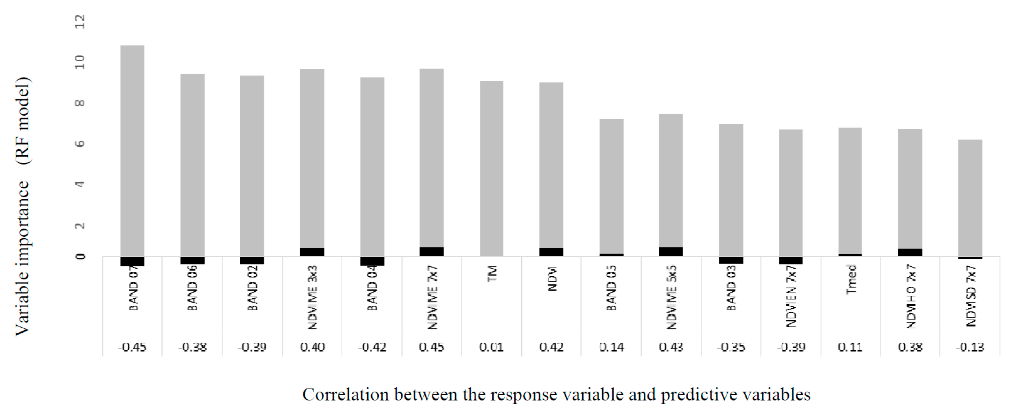
2.7.2. Random Forest (RF)

The package “randomForest” from the statistical software R [76] was utilized to construct the RF model. Candidate predictive variables were the same that considered for SVR.

The training of the RF model consisted on optimizing the parameters ntree (number of trees grown) and mtry (number of predictors sampled for spliting at each node, to minimize the influence of a very strong predictor against the other variables) [77]. The parameters mtry and ntree were optimized by evaluating their effect on the mean quadratic error. Evaluated values for Ntree were 500, 1000, 1500 and 2000, and mtry values tested were m = 3, m = 7 (m = √P), m = 15 (m = P/3) y m = 44 (m = P). Where: P = number of independent variables.

SVR and RF models were evaluated through the following goodness of fit coefficients: coefficient of determination (R²) and RMSE.

$$R^2=1-\frac{{\displaystyle {\sum }_{i=1}^n}{\left(y_i{\hat{y}}_i\right)}^2}{{\displaystyle {\sum }_{i=1}^n}{(y_i{\overline{y}}_i)}^2}$$

$$RMSE=\sqrt{\frac{{\displaystyle {\sum }_{i=1}^n}{\left(y_i-{\hat{y}}_i\right)}^2}{n-p}}$$

where:

• $y_i$ = observed AGB.
• ${\hat{y}}_i$ = predicted AGB.
• ${\overline{y}}_i$ = average AGB.
• $n$ = number of observations
• $p$ = number of model parameters.

3. Results

For SVM models, the highest model accuracy was obtained with values of cost = 4 and epsilon = 0.5, resulting in R² value of 0.80 and an RMSE of 8.2 Mg ha⁻¹. In contrast, for the default model with values of cost = 1 and epsilon = 0.1, the RMSE and R² were approximately 10 Mg ha⁻¹ and 0.68, respectively. The optimum number of support vectors were obtained from the optimized parameterization of the SVR model. The number of support vectors decreased from 273 to 170 from the model with default parameters to the optimized model.

The residuals of the default parameter and optimized parameter model are shown in Figure 2. It can be seen that none of the models had considerable limitations due to heteroscedasticity; nevertheless, the variance was more constant against the variable for the optimum parameterization model. In addition, the presence of outliers was higher in the default parameter model, with a lower prediction errors for the optimal parameterization model (Figure 2).

The evaluation of the default and optimized parameterization model allowed the predictive variables with the highest contribution to the SVR model to be identified. The variables with the highest importance both models are shown in Figure 3. Bands 7 and 4 (SWIR and NIR) were the most important variables. Average temperature (Tmed) and elevation (ELV) were selected both in the default and optimized parameterization models.

For the RF model, the optimum model accuracy was found with the following parameters: ntree= 500; mtry = 7. The default parameter model considering the 44 predictive variables, with ntree = 500 and mtry = 7, resulted in RMSE and R² of 13.62 Mg ha⁻¹ and 0.34, respectively. Figure 4 shows the variables with highest importance. The most important spectral variables were bands 7, 6 and 2; the physical variables with highest importance were maximum temperature (TM) and mean temperature (Tmed). In the process of RF optimization, a cross validation of 10 repetitions was conducted on the highest importance predictors, with the mtree and ntree obtained for model 2. The resulting reduced model with the highest importance variables shown in Figure 4 resulted in slightly improved RMSE (13.05 Mg ha⁻¹) and R² (0.40).

The analysis of residuals and predicted values against observed values is shown in Figure 5 for both the default parameter and optimized parameterization models. No important problem of variance heterogeneity could be observed for any of the models. The residual histogram was mainly symmetrical, with no problems regarding residuals normality, with the exception of a slight tendency to subestimation of the highest values.

The AGB map for the state of Durango with the model of the best fit, SVR, is shown in Figure 6. The area with the highest biomass concentration (reaching values of 55 to 168 Mg ha⁻¹) was located in the southeast of the area of study. This more dense forests corresponds to the areas with higher elevation, lower temperatures and higher precipitation. Lower biomass are observed in the more open forests at the northeast of the SMO, located in a more arid climate in transition to shrubby desert vegetation in the east of the state.

4. Discussion

The study corroborates the potential of machine-learning methods for AGB prediction and mapping as successfully utilized in recent studies (e.g., [49,51,78,79,80,81,82,83,84]). In our study, the performance of SVR was better than RF. The results of the optimized SVR model in the current study (R² = 0.80, RMSE = 8.20 Mg ha⁻¹), are higher than previous results with in the SMO with non-parametric algorithms such as regression trees [16], MP5 model trees [15] and MARS techniques [23], with R² in the range 0.5–0.7 and RMSE values of 20–38 Mg ha⁻¹ (20–40% of the average value). They also improve the previous results with SVR in the area of study with a smaller dataset of 99 plots [21], with R² of 0.62 and RMSE of 27 Mg ha⁻¹, obtaining similar results for the case of RF (R² of 0.48 and RMSE of 31 Mgha⁻¹). These goodness of fit results are also similar to those reported in the literature for AGB estimation, such as the average RMSE of 41.2 Mg ha⁻¹ (SD = 29.3 Mg ha⁻¹) reported in the review by [25], or the values of RMSE of 30–60% of the average value reported in the machine-learning studies of [19,49,82], or [83].

The better performance of SVR observed in the current study confirms the results of the previous study by [21] of a machine-learning techniques comparison in the area of study, where SVR outperformed RF and an optimal SVR parameterization was applied. It also agrees with the observations of other studies, such as the study of [82] where SVR outperformed RF, the study of [83], where SVM was the best of seven techniques including random forest and boosted regression trees, or the results from [51] or [85], where SVR was the best of 17 and 19 machine-learning techniques compared for AGB prediction, respectively. On the other hand, other studies have found RF to provide the best predictions, such as the studies by [80,81] or [86], where RF exhibited the best performance compared to neuronal networks and SVR, among other techniques. These results seems to confirm that the selection of the best method seems to be specific to the characteristics of the dataset of the area of study.

Regarding the variables’ selected in the models, the selection of band 7 (SWIR-2) as the most important variable to predict AGB from both the default parameter and optimal parameterized models, both using RF and SVR, agrees with results from previous studies where this variable has also been selected as the most important in predicting AGB [21,23] and total volume [16] in the SMO. Given the complexity of forest structure in the SMO, its inclusion seems to support the observations from several studies that vegetation indices including shortwave infrared wavelength have stronger relationships with biomass for forest sites with complex stand structures [22,87,88].

Additional bands selected by the non-parametric models, in the red and NIR domain (bands 4 and 5, respectively) and their normalized difference (NDVI) have also been found in previous studies to influence AGB [21,22,23] and several dasometric variables, including tree density and crown diameter [16] in the SMO and elsewhere [89] because of the well documented high NIR and low red reflectance in green vegetation [24,33].

In spite of the inclusion in the predictive models of the NIR band, which has been found to have a higher penetrating capacity through forested canopies [90], some subestimation of the highest AGB was observed, particularly for the RF models. The lower accuracies observed for the denser, higher biomass stands agrees with studies that have found higher accuracies in more open stands compared to denser canopy conditions (e.g., [19]). This saturation has been commonly observed in studies with Landsat imagery in areas of high biomass, generally at AGB higher than 100 Mg ha⁻¹ [6,22]. Further studies with hyperspectral sensors or in combination with light detection and ranging (LIDAR) might help improve the predictions in the areas of highest biomass.

The inclusion of textural variables both in the SVR and RF models may partially compensate some of the band saturation problems [91]. The selection of textural variables by both machine-learning techniques agrees with previous studies where textural variables have contributed to improve AGB predictions in Mexico [21,23] and elsewhere [31,91,92,93]. The texture values in an image allow the spatial heterogeneity in the different types of vegetation to be evaluated, which show distinct phenological patterns related to carbon exchange, vegetative greenness, structure and development stage [91,92]. This allows to evaluate the heterogeneity between stands through statistical models that detect a similarity within a group of contiguous pixels [93]. Because of the relative complexity in the structure of the SMO forests [52], the role of textural variables in improving AGB estimations, agrees with studies that suggest a greater role of textural variables in ecosystems with a more complex structure [22].

Elevation and temperature variables were also selected among the variables of highest importance for predicting AGB. This result agrees with previous studies that have found a role of elevation [1,12,19,29] and temperature [1,19,84] in improving remote sensing AGB predictions. For example, Yan and Wang [94] found that temperature and precipitation were the most important natural climate factors affecting the growth of vegetation in semiarid and arid regions. Propastin [95] found that the relationship between AGB and the vegetation indices significantly improved by considering elevation as a spatial weight in GWR. Similarly, Baccini [96] in their global study combining MODIS with climatic and topographic data to predict AGB, found that in areas characterized by a wide range of elevation and climate zones, climate and topography exert important control on the spatial distribution of AGB. The observed gradient from the more open, lower biomass stands in the drier eastern part of the area of study to the higher biomass in the denser stands in the colder, wetter western region of the SMO, which was captured by the models containing topographic and climatic variables, agrees with studies that have documented increasing biomass in conifer-dominated forests with increasing elevation (e.g., [19]).

Terrain features are potentially related to key features for forest stand development, such as overall climate characteristics, insolation, evapotranspiration, run-off, infiltration, wind exposure and site productivity [16,21]. Climatic and topographic variables can also affect aboveground biomass through their effects on species composition distribution and the interaction of forest species growth with different site conditions [28,30,72]. For example, Gallaun et al. [84] found in Europe that conifers had higher stocks at high altitude while the contrary occurred with broadleaves. Similarly, Powell et al. [19] found that the higher biomass ponderosa pine forests occurred at higher elevations with lower temperatures and higher precipitation. This could be consistent with our region of study, mainly dominated by pine species similar to Pinus ponderosa (e.g., Pinus duranguensis). Nevertheless, given the complexity of the species structure present in the SMO, future studies should explore the consideration of tree species abundance maps that have shown potential to improve AGB prediction in the SMO [15] and elsewhere [97].

5. Conclusions

The results of the current study demonstrated the usefulness and potential of the combination of data derived from permanent sampling plots with Landsat 8 OLI, terrain and climatic variables, to model and map AGB. For the dataset analyzed, SVM was the best method to predict AGB. With the optimization of hyperparameters (cost and epsilon) and the choice of the best kernel through cross validation, this allowed prediction error to be reduced, providing satisfactory results when dealing with large samples. The predictive variables with greater importance for the modeling of the AGB in both models were Bands 7, 4 and 2, in addition to climatic variables (mean temperature), texture variables (NDVIME3 × 3 and NDVIME7 × 7) and topographic (elevation). Future studies should consider additional vegetation and climatic variables, together with exploring the utilization of hyperspectral sensors and airborne or satellite LIDAR data, for improving AGB estimations in the area of study.

References

1. Hu, T.; Su, Y.; Xue, B.; Liu, J.; Zhao, X.; Fang, J.; Guo, Q. Mapping global forest aboveground biomass with spaceborne LiDAR, optical imagery, and forest inventory data. Remote Sens. 2016, 8, 565. [Google Scholar] [CrossRef] [Green Version]
2. Galbraith, D.; Levy, P.E.; Sitch, S.; Huntingford, C.; Cox, P.; Williams, M.; Meir, P. Multiple mechanisms of amazonian forest biomass losses in three dynamic global vegetation models under climate change. New Phytol. 2010, 187, 647–665. [Google Scholar] [CrossRef] [PubMed] [Green Version]
3. Rodríguez-Veiga, P.; Quegan, S.; Carreiras, J.; Persson, H.J.; Fransson, J.E.; Hoscilo, A.; Ziółkowski, D.; Stereńczak, K.; Lohberger, S.; Stängel, M.; et al. Forest biomass retrieval approaches from earth observation in different biomes. Int. J. Appl. Earth Obs. Geoinf. 2019, 77, 53–68. [Google Scholar] [CrossRef]
4. De Jong, W.; van Ommen, J.R. Biomass as a Sustainable Energy Source for the Future: Fundamentals of Conversion Processes; John Wiley & Sons: Hoboken, NJ, USA, 2014. [Google Scholar]
5. Morris, J. Recycle, bury, or burn wood waste biomass?: Lca answer depends on carbon accounting, emissions controls, displaced fuels, and impact costs. J. Ind. Ecol. 2017, 21, 844. [Google Scholar] [CrossRef]
6. Foody, G.M. Remote sensing of tropical forest environments: Towards the monitoring of environmental resources for sustainable development. Int. J. Remote Sens. 2003, 24, 4035–4046. [Google Scholar] [CrossRef]
7. Bunker, D.E.; DeClerck, F.; Bradford, J.C.; Colwell, R.K.; Perfecto, I.; Phillips, O.L.; Sankaran, M.; Naeem, S. Species loss and aboveground carbon storage in a tropical forest. Science 2005, 310, 1029–1031. [Google Scholar] [CrossRef] [Green Version]
8. Picard, N.; Saint-André, L.; Henry, M. Manual de Construcción de Ecuaciones Alométricas para Estimar el Volumen y la Biomasa de los Árboles: Del Trabajo de Campo a la Predicción; FAO: Rome, Italy, 2012. [Google Scholar]
9. Njana, M.A.; Meilby, H.; Eid, T.; Zahabu, E.; Malimbwi, R.E. Importance of tree basic density in biomass estimation and associated uncertainties: A case of three mangrove species in Tanzania. Ann. For. Sci. 2016, 73, 1073–1087. [Google Scholar] [CrossRef]
10. Zianis, D.; Mencuccini, M. On simplifying allometric analyses of forest biomass. For. Ecol. Manag. 2004, 187, 311–332. [Google Scholar] [CrossRef]
11. Walker, W.; Baccini, A.; Nepstad, M.; Horning, N.; Knight, D.; Braun, E.; Bausch, A. Guia de Campo para la Estimacion de Biomasa y Carbono Forestal (Field Guide to Estimate Forest Biomass and Carbon), version 1.0; Woods Hole Research Center: Falmouth, MA, USA, 2011; p. 53. [Google Scholar]
12. Asner, G.P.; Hughes, R.F.; Varga, T.A.; Knapp, D.E.; Kennedy-Bowdoin, T. Environmental and biotic controls over aboveground biomass throughout a tropical rain forest. Ecosystems 2009, 12, 261–278. [Google Scholar] [CrossRef]
13. Huang, W.; Swatantran, A.; Johnson, K.; Duncanson, L.; Tang, H.; Dunne, J.O.N.; Hurtt, G.; Dubayah, R. Local discrepancies in continental scale biomass maps: A case study over forested and non-forested landscapes in maryland, USA. Carbon Balance Manag. 2015, 10, 19. [Google Scholar] [CrossRef] [Green Version]
14. Guitet, S.; Hérault, B.; Molto, Q.; Brunaux, O.; Couteron, P. Spatial structure of above-ground biomass limits accuracy of carbon mapping in rainforest but large scale forest inventories can help to overcome. PLoS ONE 2015, 10, e0138456. [Google Scholar] [CrossRef] [PubMed]
15. López-Serrano, P.M.; López Sánchez, C.A.; Solís-Moreno, R.; Corral-Rivas, J.J. Geospatial estimation of above ground forest biomass in the Sierra Madre Occidental in the state of Durango, Mexico. Forests 2016, 7, 70. [Google Scholar] [CrossRef] [Green Version]
16. López-Sánchez, C.A.; García-Ramírez, P.; Resl, R.; Hernández-Díaz, J.C.; Lopez-Serrano, P.M.; Wehenkel, C. Modelling dasometric attributes of mixed and uneven-aged forests using Landsat-8 spectral data in the sierra madre occidental, mexico. iForest-Biogeosci. For. 2017, 10, 288. [Google Scholar] [CrossRef] [Green Version]
17. Liang, S. Recent developments in estimating land surface biogeophysical variables from optical remote sensing. Prog. Phys. Geogr. 2007, 31, 501–516. [Google Scholar] [CrossRef] [Green Version]
18. McRoberts, R.E.; Tomppo, E.O. Remote sensing support for national forest inventories. Remote Sens. Environ. 2007, 110, 412–419. [Google Scholar] [CrossRef]
19. Powell, S.L.; Cohen, W.B.; Healey, S.P.; Kennedy, R.E.; Moisen, G.G.; Pierce, K.B.; Ohmann, J.L. Quantification of Live Aboveground Forest Biomass Dynamics with Landsat Time-series and Field Inventory Data: A Comparison of Empirical Modeling Approaches. Remote Sens. Environ. 2010, 114, 1053–1068. [Google Scholar] [CrossRef]
20. Cartus, O.; Kellndorfer, J.; Walker, W.; Franco, C.; Bishop, J.; Santos, L.; Fuentes, J. A national detailed map of forest aboveground carbon stocks in Mexico. Remote Sens. 2014, 6, 5559–5588. [Google Scholar] [CrossRef] [Green Version]
21. López-Serrano, P.M.; López-Sánchez, C.A.; Álvarez-González, J.G.; García-Gutiérrez, J. A comparison of machine learning techniques applied to Landsat-5 tm spectral data for biomass estimation. Can. J. Remote Sens. 2016, 42, 690–705. [Google Scholar] [CrossRef]
22. Lu, D.; Chen, Q.; Wang, G.; Liu, L.; Li, G.; Moran, E. A survey of remote sensing based aboveground biomass estimation methods in forest ecosystems. Int. J. Digit. Earth 2014, 9, 63–105. [Google Scholar] [CrossRef]
23. López-Serrano, P.M.; Corral-Rivas, J.J.; Díaz-Varela, R.A.; Álvarez-González, J.G.; López-Sánchez, C.A. Evaluation of radiometric and atmospheric correction algorithms for aboveground forest biomass estimation using Landsat 5 tm data. Remote Sens. 2016, 8, 369. [Google Scholar] [CrossRef] [Green Version]
24. Bannari, A.; Morin, D.; Bonn, F.; Huete, A.R. A Review of Vegetation Indices. Remote Sens. Rev. 1995, 13, 95–120. [Google Scholar] [CrossRef]
25. Barbosa, J.M.; Broadbent, E.N.; Bitencourt, M.D. Remote sensing of aboveground biomass in tropical secondary forests: A review. Int. J. For. Res. 2014, 2014, 715796. [Google Scholar] [CrossRef]
26. Mohd Zaki, N.A.; Latif, Z.A. Carbon Sinks and Tropical Forest Biomass Estimation: A Review on Role of Remote Sensing in Aboveground-Biomass Modelling. Geocarto Int. 2016, 32, 701–716. [Google Scholar] [CrossRef]
27. Beaudoin, A.; Bernier, P.Y.; Guindon, L.; Villemaire, P.; Guo, X.J.; Stinson, G.; Bergeron, T.; Magnussen, S.; Hall, R.J. Mapping attributes of Canada’s forests at moderate resolution through kNN and MODIS imagery. Can. J. For. Res. 2014, 44, 521–532. [Google Scholar] [CrossRef] [Green Version]
28. Fagua, J.C.; Cabrera, E.; Gonzalez, V.H. The effect of highly variable topography on the spatial distribution of aniba perutilis (lauraceae) in the colombian andes. Rev. de Biol. Trop. 2013, 61, 301–309. [Google Scholar] [CrossRef]
29. Rana, P.; Korhonen, L.; Gautam, B.; Tokola, T. Effect of field plot location on estimating tropical forest above-ground biomass in Nepal using airborne laser scanning data. ISPRS J. Photogramm. Remote Sens. 2014, 94, 55–62. [Google Scholar] [CrossRef]
30. Van der Laan, C.; Verweij, P.A.; Quiñones, M.J.; Faaij, A.P. Analysis of biophysical and anthropogenic variables and their relation to the regional spatial variation of aboveground biomass illustrated for North and East Kalimantan, Borneo. Carbon Balance Manag. 2014, 9. [Google Scholar] [CrossRef] [Green Version]
31. Cutler, M.E.J.; Boyd, D.S.; Foody, G.M.; Vetrivela, A. Estimating tropical forest biomass with a combination of SAR image texture and Landsat TM data: An assessment of predictions between regions. ISPRS J. Photogramm. Remote Sens. 2012, 70, 66–67. [Google Scholar] [CrossRef] [Green Version]
32. Brosofske, K.D.; Froese, R.E.; Falkowski, M.J.; Banksota, A. A review of methods for mapping and prediction of inventory attributes for operational forest management. For. Sci. 2014, 60, 1–24. [Google Scholar] [CrossRef]
33. Zhang, X.; Ni-Meister, W. Remote sensing of forest biomass. In Biophysical Applications of Satellite Remote Sensing; Springer: New York, NY, USA, 2014. [Google Scholar]
34. Tonolli, S.; Dalponte, M.; Neteler, M.; Rodeghiero, M.; Vescovo, L.; Gianelle, A.D. Fusion of airborne LiDAR and satellite multispectral data for the estimation of timber volume in the Southern Alps. Rem. Sens. Environ. 2011, 115, 2486–2498. [Google Scholar] [CrossRef]
35. Rodriguez-Veiga, P.; Saatchi, S.; Tansey, K.; Balzter, H. Magnitude, spatial distribution and uncertainty of forest biomass stocks in Mexico. Rem. Sens. Environ. 2016, 183, 265–281. [Google Scholar] [CrossRef] [Green Version]
36. Straub, C.; Weinacker, H.; Koch, B. A comparison of different methods for forest resource estimation using information from airborne laser scanning and CIR orthophotos. Eur. J. For. Res. 2010, 129, 1069–1080. [Google Scholar] [CrossRef]
37. Karjalainen, M.; Kankare, V.; Vastaranta, M.; Holopainen, M.; Hyyppa, J. Prediction of plot-level forest variables using TerraSAR-X stereo SAR data. Remote Sens. Environ. 2012, 117, 338–347. [Google Scholar] [CrossRef]
38. Chen, G.; Hay, G.J.; St-Onge, B. A GEOBIA framework to estimate forest parameters from LiDAR transects, Quickbird imagery and machine learning: A case study in Quebec, Canada. Int. J. Appl. Earth Obs. Geoinf. 2012, 15, 28–37. [Google Scholar] [CrossRef]
39. Marabel, M.; Alvarez-Taboada, F. Spectroscopic determination of aboveground biomass in grasslands using spectral transformations, support vector machine and partial least squares regression. Sensors 2013, 13, 10027–10051. [Google Scholar] [CrossRef] [PubMed] [Green Version]
40. Young, T.M.; Wang, Y.; Hodges, D.G.; Guess, F.M. Decision Tree Applications for Forestry and Forest Products Manufacturers. In Proceedings of the 2008 Southern Forest Economics Workers Annual Meeting; Siry, J., Bettinger, P., Harris, T., Tye, T., Baldwin, S., Merry, K., Eds.; Center for Forest Business Publ. No. 30; University of Georgia: Athens, GA, USA, 2009; pp. 104–115. [Google Scholar]
41. Breiman, L. Random forests. Mach. Learn. 2001, 45, 5–32. [Google Scholar] [CrossRef] [Green Version]
42. Biau, G.; Scornet, E. A random forest guided tour. Test 2016, 25, 197–227. [Google Scholar] [CrossRef] [Green Version]
43. Cortes, C.; Vapnik, V. Support-vector networks. Mach. Learn. 1995, 20, 273–297. [Google Scholar] [CrossRef]
44. Garcia-Gutierrez, J.; Gonzalez-Ferreiro, E.; Mateos-Garcia, D.; Riquelme-Santos, J.C.; Miranda, D. A Comparative Study between Two Regression Methods on LiDAR Data: A Case Study. In Proceedings of the 6th International Conference on Hybrid Artificial Intelligent Systems, Wroclaw, Poland, 23–25 May 2011; Part II. pp. 311–318. [Google Scholar]
45. Chen, S.-T. Mining informative hydrologic data by using support vector machines and elucidating mined data according to information entropy. Entropy 2015, 17, 1023–1041. [Google Scholar] [CrossRef] [Green Version]
46. Drucker, H.; Burges, C.J.; Kaufman, L.; Smola, A.J.; Vapnik, V. Support vector regression machines. In Advances in Neural Information Processing Systems; MIT Press: Cambridge, MA, USA, 1997; pp. 155–161. [Google Scholar]
47. Cherkassky, V.; Ma, Y. Practical Selection of SVM Parameters and Noise Estimation for SVM Regression. Neural Netw. 2004, 17, 113–126. [Google Scholar] [CrossRef] [Green Version]
48. Wang, L.; Zhou, X.; Zhu, X.; Dong, Z.; Guo, W. Estimation of biomass in wheat using random forest regression algorithm and remote sensing data. Crop J. 2016, 4, 212–219. [Google Scholar] [CrossRef] [Green Version]
49. Shataee, S. Forest Attributes Estimation Using Aerial Laser Scanner and TM Data. For. Syst. 2013, 22, 484–496. [Google Scholar]
50. Gagliasso, D.; Hummel, S.; Temesgen, H. A comparison of selected parametric and non-parametric imputation methods for estimating forest biomass and basal area. Open J. For. 2014, 4, 42–48. [Google Scholar] [CrossRef] [Green Version]
51. García-Gutiérrez, J.; Martinez-Alvarez, F.; Troncoso, A.; Riquelme, J.C. A comparison of machine learning regression techniques for LiDAR-derived estimation of forest variables. Neurocomputing 2015, 167, 24–31. [Google Scholar] [CrossRef]
52. Wehenkel, C.; Corral-Rivas, J.J.; Hernández-Díaz, J.C.; Gadow, K. Estimating Balanced Structure Areas in multi-species forests on the Sierra Madre Occidental, Mexico. Ann. For. Sci. 2011, 68, 385–394. [Google Scholar] [CrossRef] [Green Version]
53. Corral-Rivas, J.; Vargas, B.; Wehenkel, C.; Aguirre, O.; Álvarez, J.; Rojo, A. Guía para el establecimiento de Sitios de Inventario Periódico Forestal y de Suelos del Estado de Durango; Facultad de Ciencias Forestales, Universidad Juárez del Estado de Durango: Durango, Mexico, 2009. [Google Scholar]
54. Corral-Rivas, J.; Diéguez-Aranda, U.; Corral-Rivas, S.; Castedo-Dorado, F. A merchantable volume system for major pine species in El Salto, Durango (Mexico). For. Ecol. Manag. 2007, 238, 118–129. [Google Scholar] [CrossRef]
55. Vargas-Larreta, B.; López-Sánchez, C.A.; Corral-Rivas, J.J.; López-Martínez, J.O.; Aguirre-Calderón, C.G.; Álvarez-González, J.G. Allometric equations for estimating biomass and carbon stocks in the temperate forests of north-western mexico. Forests 2017, 8, 269. [Google Scholar] [CrossRef] [Green Version]
56. Chavez, P.S. An improved dark-object subtraction technique for atmospheric scattering correction of multispectral data. Remote Sens. Environ. 1988, 24, 459–479. [Google Scholar] [CrossRef]
57. Goslee, S. Package “Landsat”. R Package Documentation. Available online: https://cran.r-project.org/web/packages/landsat/landsat.pdf (accessed on 16 December 2019).
58. Li, L.; Zhang, Q.; Huang, D. A review of imaging techniques for plant phenotyping. Sensors 2014, 14, 20078–20111. [Google Scholar] [CrossRef]
59. Huete, A.R. A Soil-Adjusted Vegetation Index (SAVI). Remote Sens. Environ. 1988, 25, 295–309. [Google Scholar] [CrossRef]
60. Zhou, J.; Guo, R.Y.; Sun, M.; Di, T.T.; Wang, S.; Zhai, J.; Zhao, Z. The effects of glcm parameters on lai estimation using texture values from quickbird satellite imagery. Sci. Rep. 2017, 7, 7366. [Google Scholar] [CrossRef] [PubMed]
61. PCI Geomatics; PCI Geomatics Inc.: Toronto, ON, Canada, 2013.
62. INEGI. Continuo de Elevaciones Mexicano 3.0; Instituto Nacional de Estadística y Geografía: Aguascalientes, Mexico, 2013.
63. Fleming, C.; Giles, J.; Marsh, S. Elevation Models for Geoscience; Geological Society of London: London, UK, 2010. [Google Scholar]
64. Horning, N. Remote Sensing for Ecology and Conservation: A Handbook of Techniques; Oxford University Press: Oxford, UK, 2010. [Google Scholar]
65. INIFAP. Red nacional de estaciones agroclimáticas automatizadas (RNEAA). Instituto Nacional de Investigaciones Forestales, Agrícolas y Pecuarias. Available online: https://clima.inifap.gob.mx/lnmysr (accessed on 16 December 2019).
66. Oliver, M.A.; Webster, R. Kriging: A method of interpolation for geographical information systems. Int. J. Geogr. Inf. Syst. 1990, 4, 313–332. [Google Scholar] [CrossRef]
67. Clark, P.J.; Evans, F.C. Distance to nearest neighbor as a measure of spatial relationships in populations. Ecology 1954, 35, 445–453. [Google Scholar] [CrossRef]
68. Horn, B.K. Hill shading and the reflectance map. Proc. IEEE 1981, 69, 14–47. [Google Scholar] [CrossRef] [Green Version]
69. Zevenbergen, L.W.; Thorne, C.R. Quantitative analysis of land surface topography. Earth Surf. Process. Landf. 1987, 12, 47–56. [Google Scholar] [CrossRef]
70. Moore, I.D.; Grayson, R.; Ladson, A. Digital terrain modelling: A review of hydrological, geomorphological, and biological applications. Hydrol. Process. 1991, 5, 3–30. [Google Scholar] [CrossRef]
71. McCune, B.; Keon, D. Equations for potential annual direct incident radiation and heat load index. J. Veg. Sci. 2002, 13, 603–606. [Google Scholar] [CrossRef]
72. Stage, A.R. An expression for the effect of aspect, slope, and habitat type on tree growth. For. Sci. 1976, 22, 457–460. [Google Scholar]
73. Awad, M.; Khanna, R. Efficient Learning Machines: Theories, Concepts, and Applications for Engineers and System Designers; Apress: New York, NY, USA, 2015. [Google Scholar]
74. Yu, P.-S.; Chen, S.-T.; Chang, I.-F. Support vector regression for real-time flood stage forecasting. J. Hydrol. 2006, 328, 704–716. [Google Scholar] [CrossRef]
75. Meyer, D.; Dimitriadou, E.; Hornik, K.; Weingessel, A.; Leisch, F. Package ‘e1071’. 2017. Available online: https://cran.r-project.org/web/packages/e1071/e1071.pdf (accessed on 26 January 2018).
76. RColorBrewer, S.; Liaw, A.; Wiener, M.; MLiaw, A. Package ‘randomForest’. 2018. Available online: https://cran.r-project.org/web/packages/randomForest/randomForest.pdf (accessed on 16 December 2019).
77. Möller, A.; Tutz, G.; Gertheiss, J. Random forests for functional covariates. J. Chemom. 2016, 30, 715–725. [Google Scholar] [CrossRef]
78. Ni, X.; Cao, C.; Zhou, Y.; Ding, L.; Choi, S.; Shi, Y.; Park, T.; Fu, X.; Hu, H.; Wang, X. Estimation of forest biomass patterns across northeast china based on allometric scale relationship. Forests 2017, 8, 288. [Google Scholar] [CrossRef] [Green Version]
79. Shen, W.; Li, M.; Huang, C.; Wei, A. Quantifying live aboveground biomass and forest disturbance of mountainous natural and plantation forests in northern guangdong, china, based on multi-temporal Landsat, Palsar and field plot data. Remote Sens. 2016, 8, 595. [Google Scholar] [CrossRef] [Green Version]
80. Baccini, A.; Laporte, N.; Goetz, S.J.; Sun, M.; Dong, H. A First Map of Tropical Africa’s Above-ground Biomass Derived from Satellite Imagery. Environ. Res. Lett. 2008, 3, 045011. [Google Scholar] [CrossRef] [Green Version]
81. Vafaei, S.; Soosani, J.; Adeli, K.; Fadaei, H.; Naghavi, H.; Pham, T.D.; Bui, D.T. Improving accuracy estimation of Forest Aboveground Biomass based on incorporation of ALOS-2 PALSAR-2 and Sentinel-2A imagery and machine learning: A case study of the Hyrcanian forest area (Iran). Remote Sens. 2018, 10, 172. [Google Scholar] [CrossRef] [Green Version]
82. Gleason, C.J.; Im, J. Forest biomass estimation from airborne LiDAR data using machine learning approaches. Remote Sens. Environ. 2012, 125, 80–91. [Google Scholar] [CrossRef]
83. Li, M.; Im, J.; Quackenbush, L.J.; Liu, T. Forest Biomass and Carbon Stock Quantification Using Airborne LiDAR Data: A Case Study Over Huntington Wildlife Forest in the Adirondack Park. IEEE J. Sel. Top. Appl. Earth Observ. Remote Sens. 2014, 7, 3143–3156. [Google Scholar] [CrossRef]
84. Gallaun, H.; Zanchi, G.; Nabuurs, G.-J.; Hengeveld, G.; Schardt, M.; Verkerk, P.J. Eu-wide maps of growing stock and above-ground biomass in forests based on remote sensing and field measurements. For. Ecol. Manag. 2010, 260, 252–261. [Google Scholar] [CrossRef]
85. Jachowski, N.R.; Quak, M.S.; Friess, D.A.; Duangnamon, D.; Webb, E.L.; Ziegler, A.D. Mangrove biomass estimation in Southwest Thailand using machine learning. Appl. Geogr. 2013, 45, 311–321. [Google Scholar] [CrossRef]
86. Wu, C.; Huanhuan, S.; Aihua, S.; Jinsong, D.; Muye, G.; Jinxia, Z.; Hongwei, X.; Ke, W.J. Comparison of machine-learning methods for above-ground biomass estimation based on Landsat imagery. J. Appl. Remote Sens. 2016, 10, 035010. [Google Scholar] [CrossRef]
87. Freitas, S.R.; Mello, M.C.S.; Cruz, C.B.M. Relationships between forest structure and vegetation indices in Atlantic Rainforest. For. Ecol. Manag. 2005, 218, 353–362. [Google Scholar] [CrossRef]
88. Pizaña, J.M.G.; Hernández, J.M.N.; Romero, N.C. Remote sensing-based biomass estimation. In Environmental Applications of Remote Sensing; IntechOpen: London, UK, 2016. [Google Scholar]
89. Trotter, C.M.; Dymond, J.R.; Goulding, C.J. Estimation of timber volume in a coniferous plantation forest using Landsat TM. Int. J. Remote Sens. 1997, 18, 2209–2223. [Google Scholar] [CrossRef]
90. Huete, A.; Liu, H.; van Leeuwen, W.J. The Use of Vegetation Indices in Forested Regions: Issues of Linearity and Saturation. In Proceedings of the 1997 IEEE International Geoscience and Remote Sensing Symposium Proceedings. Remote Sensing—A Scientific Vision for Sustainable Development, Singapore, 3–8 August 1997; pp. 1966–1968. [Google Scholar]
91. Kelsey, K.C.; Neff, J.C. Estimates of Aboveground Biomass from Texture Analysis of Landsat Imagery. Remote Sens. 2014, 6, 6407–6422. [Google Scholar] [CrossRef] [Green Version]
92. Wood, E.M.; Pidgeon, A.M.; Radeloff, V.C.; Keuler, N.S. Image texture as a remotely sensed measure of vegetation structure. Remote Sens. Environ. 2012, 121, 516–526. [Google Scholar] [CrossRef]
93. Nichol, J.E.; Sarker, M.L.R. Improved biomass estimation using the texture parameters of two high-resolution optical sensors. IEEE Trans. Geosci. Remote Sens. 2011, 49, 930–948. [Google Scholar] [CrossRef] [Green Version]
94. Yan, F.; Wu, B.; Wang, Y. Estimating spatiotemporal patterns of aboveground biomass using Landsat TM and MODIS images in the Mu Us Sandy Land, China. Agric. For. Meteorol. 2015, 200, 119–128. [Google Scholar] [CrossRef]
95. Propastin, P. Modifying geographically weighted regression for estimating aboveground biomass in tropical rainforests by multispectral remote sensing data. Int. J. Appl. Earth Obs. Geoinf. 2012, 18, 82–90. [Google Scholar] [CrossRef]
96. Baccini, A. Forest biomass estimation over regional scales using multisource data. Geophys. Res. Lett. 2004, 31. [Google Scholar] [CrossRef] [Green Version]
97. Yang, C.; Huang, H.; Wang, S. Estimation of tropical forest biomass using Landsat TM imagery and permanent plot data in Xishuangbanna, China. Int. J. Remote Sens. 2011, 32, 5741–5756. [Google Scholar] [CrossRef]
Figure 1. Location of the area of study and of the permanent forestry and soil research sites (SPIFyS in Spanish). Temperate forest distribution source is Instituto Nacional de Estadística y Geografía (INEGI) Land-Use Map Series V.
Forests 11 00011 g001
Figure 2. Predicted against observed aboveground biomass (Mg ha−1) and distribution of residuals against predicted biomass of the support vector regression (SVR) model for the default parameterization (left) and for the optimized parameterization (right).
Forests 11 00011 g002
Figure 3. Variable importance for the for the default parameterization (left) and for the optimized parameterization (right) SVR models. Grey bars represent variable importance and black bars represent the correlation between the response variable and predictive variables.
Forests 11 00011 g003
Figure 4. Relative importance of predictive variables in the random forest (RF) model. Grey bars represent variable importance and black bars represent the correlation between the response variable and predictive variables.
Forests 11 00011 g004
Figure 5. Prediction of the RF model and distribution of residuals against observed AGB (Mg ha−1) for the default parameterization (left) and for the optimized parameterization (right).
Forests 11 00011 g005
Figure 6. Predicted of aboveground biomass (Mg ha−1) in the Durango Sierra Madre Occidental (SMO) generated from the best fit SVR model.
Forests 11 00011 g006