Article

Automated Cable Road Layout and Harvesting Planning for Multiple Objectives in Steep Terrain

by
Leo Gallus Bont
1,*,
Sabrina Maurer
2 and
Jochen Ruben Breschan
2
1
Swiss Federal Institute for Forest, Snow and Landscape Research (WSL), Forest Production Systems Group, Zuercherstrasse 111, CH 8903 Birmensdorf, Switzerland
2
Department of Environmental Systems Science, ETH Zurich, 8092 Zurich, Switzerland
*
Author to whom correspondence should be addressed.
Forests 2019, 10(8), 687; https://doi.org/10.3390/f10080687
Submission received: 4 July 2019 / Revised: 31 July 2019 / Accepted: 13 August 2019 / Published: 14 August 2019
(This article belongs to the Special Issue Forest Operations in Environmentally Sensitive Areas)

Abstract

:
Cable yarding is the most commonly used technique for harvesting timber from steep terrain in central Europe. During the planning process, one important task is to define the cable road layout. This means that the harvesting technology and cable road location must be specified for a given timber parcel. Although managers must minimize harvesting costs, it is even more important that such work on forests reduces the potential for damage to the residual stand and ensures that environmental conditions remain suitable for regeneration. However, current methods are geared only toward minimizing harvesting costs and are computationally demanding and difficult to handle for the end user. These limitations hinder broad application of such methods. Further, the underlying productivity models used for cost estimation do not cover all conditions of an area and they cannot be applied over a whole harvesting area. To overcome these shortcomings, we present: (1) a multiobjective optimization approach that leads to realistic, practicable results that consider multiple conflicting design objectives, and (2) a concept for an easy-to-use application. We compare the practical applicability and performance of the results achieved with multiobjective optimization with those achieved with single-objective (cost-minimal) optimization. Based on these points, we then present and discuss a concept for a user-friendly implementation. The model was tested on two sites in Switzerland. The study produced the following major findings: (1) Single-objective alternatives have no practical relevance, whereas multiobjective alternatives are preferable in real-world applications and lead to realistic solutions; (2) the solution process for a planning unit should include analysis of the Pareto frontier; and (3) results can only be made available within a useful period of time by parallelizing computing operations.

1. Introduction

Forests on steep terrain, in particular in densely populated areas such as in the European Alps, are managed for multiple objectives and purposes [1]. They provide services and goods such as raw material (timber, fuel wood), biodiversity, and recreation, and they protect infrastructure against gravitational natural hazards such as landslides, avalanches, flooding, and rock fall [2]. In almost all cases, forest management is the most efficient way to provide these goods and services, even if the forest operation itself is not economical. Therefore, even forests in steep terrain with high harvesting costs are managed. For these, mountain forests cable-based technologies have been the backbone of harvesting [3].
From an operational point of view, an important step and a challenging task is to determine the spatially explicit layout of a set of cable roads (CR) or a harvesting layout over a given area. This means that the technology and the location of CRs must be specified for each timber parcel TP (we defined ‘timber parcel’, or TP, as the smallest harvestable unit, here being 10 m × 10 m). A harvesting or CR layout has to fulfill several objectives: the operation should be cost efficient, but also reduce the potential for damage to the residual stand and ensure that the regeneration finds suitable conditions [4].
The first decision support system for designing CR layouts was developed by Dykstra and Riggs [5]. With this approach, cost-minimal logging units could be identified. Later, Chung and Sessions [6] and Chung et al. [7] described a combined method for cable logging operation and road network planning. However, those approaches, developed in North America, were particularly tailored to clear-cut conditions, and the latter relied on heuristic solution finding. Bont et al. [4] presented a model that was particularly tailored to central European conditions. However, this model formulation was not able to solve real-size problems. This shortcoming was later addressed by Bont and Church [8], who presented an approach inspired by location set covering. They developed two computationally efficient models: a set-covering model (SCM) and a bounded set-covering model (BSCM). These models are tailored to harvesting techniques under central European conditions. However, the models are geared only toward minimizing harvesting costs and do not factor in the target of minimizing negative impacts on the remaining forest or the environment, necessary aspects of multifunctional managed forests. In addition, the approach presented by Bont and Church [8] is still computationally demanding and relies on commercial solvers that are expensive for the end user, which limits its applicability.
Further, the underlying productivity models used for cost estimation do not cover all conditions of an area and they cannot be applied over a whole harvesting area. This is caused by the fact that productivity models have mostly been developed under more or less ideal conditions of use to answer specific research questions (e.g. [9]). For this reason, they are not appropriate for mapping patterns under non-ideal conditions of use. For example, CRs that run (nearly) horizontally to a slope are considered unfavorable and usually avoided in practice because of low productivity or ergonomic aspects [10,11]. As such situations rarely occur in the data underlying productivity models, the variables that may best describe such situations are not identified as significant and therefore are not included in the model. One option to solve this problem could be to develop productivity models with a broader range of application. This would require a digitalization of cable yarders and chainsaw-based harvesting operations similar to the systems already implemented in harvester-based operations [12]. The implementation of such resources might require a lot of resources and considering the rather small area of application, this will not be a priority of forest operations research. Another easier solution to deal with these shortcomings is to identify such unfavorable situations and incorporate them as a separate objective, which must be minimized, in the model. This second strategy is applied and discussed in this paper.
Specifically, we present: (1) a multiobjective optimization approach, which avoids unfavorable CRs and therefore leads to realistic, practicable results, and (2) a concept for an easy-to-use application, which can also be operated by a user with no knowledge of programming and modelling that derives automatically a pareto set of optimal solutions and that does not require expensive purchases of software. We compare the practical applicability and performance of the results achieved by multiobjective optimization with those achieved by single-objective (cost-minimal) optimization. Based on these points, we then present and discuss a concept for a user-friendly implementation.

2. Methods

2.1. Conceptual Model

Our conceptual model (Figure 1) is a further development of the SCM/BSCM model proposed by Bont and Church [8], extended with a component that maps the negative impact of a CR. Additionally, the wood-harvesting process is captured from standing trees to a virtual pile at the interface of the planning unit. Thus, our conceptual model comprises three subsystems: (1) “Harvesting System”, creating a set of feasible CRs and harvesting alternatives to access TPs; (2) “Harvesting Cost”, assessing the economic efficiency of harvesting techniques; and (3) “Negative Impact”, evaluating the negative effects of the harvesting operation on regeneration, the remaining stand, and ergonomic aspects (Figure 1). The subsystems “Harvesting System” and “Harvesting Cost” were already discussed in [4,8] and are not presented again here.
To provide geographical information, we use a database, represented as a 10-m spaced raster, with four layers: (1) digital elevation model, (2) volume of timber to harvest, (3) obstacles for cable yarding (e.g., high-voltage power lines), and, if available, (4) the positions of trees that are appropriate for use as intermediate supports. An additional layer for any qualified landings (or forest roads) is imported as a vector-defined dataset.

2.2. Multiobjective Optimization

The approach presented here aims to optimize several objectives concurrently, and the concept of “multiobjective optimization” is therefore briefly introduced in this section. Real-world environmental optimization problems are in most cases multiobjective because they have several, in most cases contradictory, goals that must be met at the same time [13]. There is seldom a single strategy that optimizes all objective functions simultaneously. Most optimization algorithms are based on a scalar fitness function that controls the search. One of the most intuitive approaches is to bring together the different objectives into a single function using the weighted sum of objective function methods [14]. Weighting factors represent the priorities and can be assigned in two ways: (1) a priori, where the trade-offs to be applied are defined before the optimization methods are performed, and (2) a posteriori, where the decision-maker chooses the solution by exploring possible options calculated by optimization methods [15]. A posteriori methods generate a trade-off surface at the end of the optimization process.
By varying the value of the weights, it is possible to approximate the trade-off surface. One obvious problem with this approach, however, is that it may be difficult to generate a set of weights that properly scales the objectives when little is known about the problem. Another drawback is that this approach cannot generate mathematically appropriate members of the Pareto [16] optimal set when the frontier is concave [15,17].
Examples of multiobjective optimization approaches in forest engineering and operations were described by Stueckelberger et al. [18], Kanzian et al. [19] and Hosseini at al. [20]. Stueckelberger et al. [18] described a three-objective optimization problem for automatic road network planning. They addressed the objectives of construction and maintenance costs, negative ecological effects, and the suitability for cable-yarding landings. Further, effects of this multiobjective problem on Pareto-optimal solutions were observed. Kanzian et al. [19] optimized the design of forest energy supply networks by using multiobjective optimization. The objectives were to maximize profit and minimize CO2 emissions. In addition, the Pareto set of optimal solutions was observed. Hosseini et al. [20] presented a holistic optimization framework for forest machine trail network design. Economic and ecological objectives involved in designing machine trail networks were considered and the Pareto frontier was analyzed.

2.3. Mathematical Formulation

In a previous paper [8], we presented the set-covering model (SCM) and the bounded set-covering model (BSCM) and demonstrated that these models are computationally efficient model formulations and that the two models are equivalent in terms of quality of the results and computational efficiency. We used these models for single-objective optimization. We now adapt the SCM model for multiobjective optimization. The multiobjective set-covering model (MSCM) is formulated as follows:

2.3.1. Notation

x i H
 = 1 if TP i is harvested by the lowest-cost harvesting alternative to yarding (winch or helicopter), = 0 otherwise.
v i H
 value of TP i (=selling price of the timber minus cost of harvesting (variable cost)) that is harvested by the lowest-cost harvesting alternative to a CR (in Swiss Francs, CHF).
x i c
 = 1 if parcel i is harvested by a section k of a set of clustered roads ( k   M i c ), = 0 otherwise.
v i c
 value of TP i (=selling price of the timber minus variable harvesting cost) that is harvested by section k   M i c , v i c = k v i k v i k for k   M i c (mean value).
v i k
 value (in CHF) of TP i (=selling price of the timber minus cost of harvesting (variable cost)) that is harvested over CR section k.
n c i
 Number of clusters for parcel i.
y k
 = 1 if CR section k is built, = 0 otherwise.
f k c
 Cost (in CHF) of installing CR section ( k   L l , m or cost of extending a CR section from section   b   P k , where b is the section that precedes section k.
c 
 index of cluster for corresponding TP i.
M i c
 = (k | CR section k can reach TP i and is associated with cluster c in parcel i).
f k S L
 Penalty value of that part of CR section k that is on a slope line steeper than 25° and in unfavorable direction compared with the slope line.
f k D H
 Penalty value to penalize downhill logging: horizontal length (m) of CR section k that is steeper than 10° and built for down-hill logging.

2.3.2. Objectives

The objectives of the multiobjective model are the following: (1) to maximize net revenue, which is calculated as the selling price of the wood minus harvesting costs, including those for installing CRs, plus those that vary according to cable or alternative harvesting technologies (Equation (1)) (we have cast the objective in an equivalent minimization form, where each term in the objective is multiplied by minus one.); (2) to minimize the impact of unfavorable CR directions in terms of silviculture, worker safety or natural hazards (negative impacts) (Equation (2)); and (3) to minimize the length of downhill logging (Equation (3)). Constraints are the same as in [8] and are not listed here. yk is the only binary integer variable, xic and xiH are continuous variables, which can take values between 0 and 1.
Min : Z C = c n c i i v i c x i c + k f k C y k i v i H X i H
Z S L = k f k S L y k
Min : Z D H = k f k D H y k

2.3.3. Scaling

Problems that have multiple criteria to be fulfilled in their objectives are often solved by combining all components into one scalar objective function, then minimizing the weighted sum of this aggregated function. To make these single-objective functions comparable, one must scale the data. As our data are normally distributed, we chose a normalization [21]. The combined weighted objective function (Equation (4)) is defined in the equation above with weights λC for ZC (cost), λSL for ZSL (slope line), and λDH for ZDH (downhill).
Min :   Z o v e r a l l = λ C Z C + λ S L Z S L + λ D H Z D H

2.4. Harvesting System

The harvesting system module evaluates all possible harvesting options for all TPs and estimates the cost of these options. As a result, one knows for each TP which landings can be reached with which harvesting system and which CR section. A landing is located on the forest road and represents the interface between the terrain transport and the on-road transport and offers favorable conditions for the installation of a cable yarder, particularly due to the presence of anchor trees and enough work space. The harvesting systems are subdivided into cable yarders and alternative harvesting technologies such as helicopters or winches.
TPs that can be accessed with cable yarders are identified on the basis of the modelling of individual CRs. We assume that from every potential landing a CR can be built in all directions. The feasibility of each CR and the maximum line length are checked for each line on the basis of the topography and cable mechanical parameters. The procedure was outlined in detail in [4]. The maximum line length is limited by the length of the cable, by obstacles within the length profile and by the physical feasibility (payload, required ground clearance, topography of the terrain). An obstacle is an object over which no skyline can be spanned, such as buildings, high-voltage power lines, cable cars, railway lines or important roads. Since the topography is checked for each single CR, ridges are also detected.
For each TP there is also the option of using an alternative harvesting system, winches can typically be used in the proximity of roads, otherwise helicopter harvesting is considered as an alternative. If the harvest with a winch is possible, only the winch can be considered as an alternative to the use of a cable yarder.
We require that all TPs are harvested either by cable yarder or an alternative harvesting system. The expense incurred with the harvesting alternative could also serve as an upper marginal cost for harvesting a unit via cable yarding.

2.5. Optimization Objectives

In regions such as the Alps, where forests must be managed for a mixed set of goods and services (including protection against natural hazards), particular constraints are necessary during logging operations. When cutting old trees, the overall objective is to promote the regeneration of a healthy forest. Therefore, it is important to minimize the negative impact of harvesting on the residual stand or potential regeneration. In most cases, that is more important than cost efficiency. The negative impact of harvesting is considered by the objectives “unfavorable CR direction” and “downhill logging” which are presented hereafter. However, the cases described here are not final. Another negative impact of harvesting could be that the wood touches the ground during logging and damages the soil. This could also be included as a separate objective. In our case, however, only CRs that have sufficient ground clearance are considered and therefore no soil damage is caused by cable logging, which corresponds to current practice in Switzerland.

2.5.1. Harvesting Costs

The first objective in planning is to maximize revenue from the cut wood. For this aim, all principal cost elements of harvesting must be estimated. This includes fixed costs, such as for the set-up and dismantling of the yarding system.
The other expense category is variable costs, such as felling, cable-based extraction from the parcel to the forest road, processing of the trees, and hauling the logs to a virtual pile. The productivity and the costs model used here were described in [8].

2.5.2. Minimize Impact of Unfavorable CR Directions

The emergence of gravitational natural hazards depends on the slope and the length of an aisle in the forest [22]. Therefore, forest aisles in unfavorable slope line directions should be avoided in steep terrain. This includes aisles that are required to set up and run a cable yarder. An aisle in the direction of the slope line bears the risk of avalanches, snow creep, landslides and rock fall. All of these risk processes become valid at a slope of 25 to 30° [22,23]; if one of these risks materializes, tree growth is either hindered or made impossible. To accommodate regeneration, expensive technical solutions (e.g., snow fences) are required. For example, as shown in Table 1, avalanches can be activated starting at slopes of 30°. The longer the aisle, the lower the slope inclination required to start the process.
A CR that runs diagonally to the slope line can also be advantageous because it benefits landscape aesthetics, deflects negative impacts on residual trees, and enhances worker safety [10]. Aggeler [10] indicated that in the case of cable lines that run parallel to the slope line, slipping logs and stones endanger personnel and equipment. This risk is reduced for CRs that are oriented diagonally to the slope. In the case of CRs running parallel to the slope, the risk of damages to the remaining stand increases with steeper slopes. This is due to the diagonal feed of the timber to the skyline. In the case of CRs running diagonally to the slope, the timber is fed in along the slope line. This means that, even with longer feeds on the downhill side, the timber can be harvested with a lower risk of damaging the remaining stand [10]. A study on the influence of the direction of the CR in relation to the slope line came to a similar conclusion, i.e. that trees within a distance of 7.5 m from the skyline suffer less damage with slope-diagonal lines than with slope-parallel lines [24]. Furthermore, CRs installed parallel to the slope line are more visible in the scenery, which lowers the social acceptance of timber harvesting operations [10].
Although CRs that run diagonal (usually around 35°–45° deviation) to the slope have some advantages for cable logging, CRs with a larger deviation of 35°/45°–90° are quite rare, as such unfavorable CR directions are usually avoided in practice because of low productivity or ergonomic aspects [10,11]. Therefore, productivity models that are valid for such situations are not available and studies quantifying negative impacts on the environment and worker safety could not be found. We, therefore, assume that CRs with a deviation greater than about 45° from the slope line direction should be avoided and penalized. The threshold of 45° is based on expert experience.
The implementation of this objective is done by comparing the slope-line direction of each grid cell with the direction of the overlaying CR. For this purpose, we compare the direction of the CR with the slope line at intervals of 10m on each CR section. A specific penalty value is then introduced for different deviations, such as applied in Table 2. This penalty value was computed for each point on the 10m interval and summed for each individual CR section. The penalty value depends on the angle of deviation of the slope line from the CR direction and the length of the CR in this range. However, it is difficult to quantify an optimal angle of deviation because it depends on the properties of the project site and should be determined together with people with local knowledge.

2.5.3. Minimize Downhill Logging

Yarding of whole trees downhill significantly increases the risk of injury to the remaining stand compared with yarding uphill [24,25]. Therefore, the former method is rarely applied. If downhill yarding is required, a cut to length system is recommended, a practice that generally causes less damage but increases cost. By doing so, downhill logging is already penalized in the decision model.
If it is not clear whether whole tree systems will also be used for downhill logging, or if a forest enterprise tries to maximize the area that can be covered by whole tree systems (e.g. for ergonomic reasons), it can make sense to penalize downhill logging. In this case, the horizontal length must be minimized for any cable that is proposed for downhill logging and on slopes steeper than a certain threshold. Here, we use a 10° threshold to distinguish downhill from flat terrain. Only parts of the CR where the inclination is steeper than 10° are penalized.

2.6. Compute the Pareto Frontier

Multiobjective optimization was first described by Pareto [16] and Edgeworth [26]. A feasible solution to a multiobjective problem is considered Pareto-optimal if no objective component can be improved upon without worsening one or more of the other components [27]. Our determination of the Pareto frontier (tri-objective optimal alternatives) was based upon step-wise changes in the relative weight of objective-function parameters λ. The solutions were controlled only by the direction of the weighting vector λ, and values for λSL, λDH and λC were varied.

2.6.1. Concept of Relative Negative Impact for Three Objective Alternatives

To analyze and map the trade-off between harvesting costs [CHF/m3] and the negative impact from objectives “unfavorable CR direction” and “downhill logging”, we introduced the concept of relative negative impact. Objectives “unfavorable CR direction” and “downhill logging” were merged to create a combination we designated as the negative impact (NI). We also calculated a relative negative impact (RNI). The NI corresponded to the scaled objective function of those objectives, while the RNI mapped deviations to the worst damage found in all potential solutions when various scaled solutions were evaluated (e.g., analysis of Pareto frontier). We defined Equations (5) and (6), where max (NI) was the damage potential for the cost-optimal solution (λSL = 0, λDH = 0, λC = 1).
Min :   N I   =   w S L × Z S L +   w D H × Z D H
R N I   =     N I × 100 max ( N I )

2.6.2. NISE Approach for Two Objective Alternatives

For the problem of CR layout planning, it might not be necessary to deal with three objectives. The objective “downhill logging” could be dropped, as explained in the section “minimize downhill logging”, and two objectives might be enough. When running a two-objective optimization, the NISE approach described below can be applied.
The NISE approach is used to generate an approximate or an exact representation of the Pareto set for problems with two objectives [28]. The approach proceeds by iteratively adding solutions to the Pareto set until a maximum allowable error is no longer violated. The weight combinations for new solutions result from the slopes when the points of the current Pareto set are connected. A major innovation is the computation of the maximum possible error, which the analyst may control, to obtain an approximation for a desired degree of accuracy [28], as shown in Figure 2.

2.7. Procedure for the Automatic Derivation of a CR Layout

To automatically derive the CR layout for a perimeter of practical size, we followed the steps described below:
  • (I) Preparation of the geoinformation relevant for planning: (a) development including machine locations, (b) topography, (c) obstacles and (d) wood occurrence.
  • (II) Classification into processing areas: The perimeter is divided into smaller processing areas to reduce computing time, which increases proportionally with the processed area and can reach values in the order of days. Classification is usually done in consideration of transport boundaries (e.g., road) and obstacles (e.g., power line). Where areas that are too large occur, despite consideration of the aforementioned elements, they are artificially separated into smaller sub-areas. Here, additional artificial boundaries are added that are guided by the slope line.
  • In each processing area, steps [III] and [IV] are then applied:
  • (III) Creation of potential CRs: Based on the potential machine locations and the topography, a set of feasible CRs is automatically calculated. Potential CRs in different directions and different lengths are automatically planned at each machine location. This automatic planning identifies the optimal intermediate support layout with regard to ground clearance and under the assumption of a certain payload, such as defined in Table 3. The description of the cable mechanics is based on the Pestal method, which is suitable because of its short computing time.
  • (IV) Derivation of the CR layout: From the previously created set of feasible CRs, the subset of CRs that optimally cover the areas with wood occurrences is automatically selected. The covered area of a CR is determined using the working field width. “Optimal” means that the design objectives for the CR layout have been met in the best possible way. In addition to the cable yarder as a means of harvesting, the winch and the helicopter are also available. They are used where the design objectives can be achieved better than with the cable yarder. The helicopter also covers areas that cannot be reached with the cable yarder.
  • (V) Summary of the CR layouts: The CR layouts for the processing areas derived in step [IV] are summarized over the entire perimeter.

3. Model Application

The purposes of our model application are twofold. First, we compare the practical applicability and performance of the results achieved by multiobjective optimization with those achieved by single-objective optimization (cost-minimal solution). This is done for harvesting units in the Rigi area in Weggis, Switzerland. Second, we evaluate the incorporation of the NISE method for computing the Pareto frontier in terms of computational efficiency and quality of the results. This is done for the Gotschna area in Klosters, Switzerland.

3.1. Project Areas and Properties

3.1.1. General Properties

The parameters of the harvesting techniques are displayed in Table 3. In both project sites the main harvesting technique is the cable yarder. In Gotschna two types of cable yarders are used, one with a maximum diagonal length of 600 m and one with a maximum diagonal length of 800 m, whereas in Rigi only one cable yarder type is used. The productivity models were calibrated with the experience values listed in Table 3, and as described in [8].
For both project sites, spatial information was not available about trees that might be appropriate for use as intermediate supports. Therefore, we assumed that the cost of rigging an intermediate support would not depend on its exact spatial position. Possible landing positions were identified and reported by the local forest authorities. The spatial resolution of the raster grid was 10 m × 10 m for Rigi and 15 m × 15 m for Gotschna. A more detailed description of the project site is given in the subsequent sections.
We generated our models in MATLAB R 2016 and solved each model using the Gurobi 7.0.1 optimization package (Gurobi GmbH, Bad Homburg, Germany). We used an Intel® Core™ i7-6700 CPU with 3.4 GHz and 16 GB RAM (Fujitsu, Tokyo, Japan). The reported computation times refer only to the optimization part with GUROBI (real time). The optimization model for the Gotschna area was set up and solved using the EULER (Hewlett-Packard, Palo Alto, USA) computing cluster at ETH Zurich (Intel Xeon E5-2697v2 processors (2.7 GHz nominal, 3.0–3.5 GHz peak)).

3.1.2. Rigi

The Rigi project site is located on the slopes of the Rigi mountain in the canton of Lucerne in central Switzerland (UTM Coordinates: 47.039, 8.447). This region is characterized by steep terrain, with an average slope gradient >30°, and a forest that provides a variety of services, such as wood production and protection against natural hazards (avalanches, rock fall, landslides). Therefore, it is an ideal study site for investigating scenarios with multiple, conflicting objectives.
Only one yarding system was considered—a tower yarder with a maximum cable length of 1000 m. The harvest width of the CR was not constant, but between 50 m and 70 m as displayed in Figure 3. Aggeler [10] showed that larger distances between cable lines are possible with cable lines that run diagonal to the slope. Six sub-areas were selected. Their properties, such as size, and the number of variables considered are listed in Table 2. The idea behind defining different types of sub-areas (with different sizes and complexities) was to determine until which size and number of variables it is possible to solve the optimization problem. The sub-areas are visualized in Figure 4. Note that the landings and the forest road at the bottom right in Figure 4 have a limited bearing capacity, which leads to additional trans-shipment costs of 15 CHF/m3 for these landings.
Optimization procedures were applied to three objectives: minimize the cost, minimize the CR length in slope line direction and minimize the CR length in an unfavorable direction. For the last objective, the optimal deviation of the CR direction from the slope line was between 10° and 35° (Table 2). We took a weighted sum approach (Equation 4) to find multiobjective-optimal solutions that were controlled by only the direction of the weighting vector λ. The weights of λ were varied to (0, 0.25, 0.5, 0.75, 1), which produced 15 alternatives. We let λSL + λDH + λC = 1. For our evaluation, all alternatives considered costs because alternatives without a cost had no practical relevance. Therefore, λC always had a positive value. We replaced cases of λC = 0 with λC = 0.02.
A volume map provided by the local forest authorities was used to estimate the amount of wood to harvest, which was assigned to a 10 m × 10 m raster map. The procedure then followed the steps outlined in Figure 5. The harvesting was limited to forests with stocks ≥ 300 m3/ha. The annual increment was estimated at 6 m3/ha/y and extrapolated to a recurrence interval of 20 years. The intervention was assumed to have a value of 30%, based on [29]. In the Rigi area in particular, when the helicopter was chosen as the harvesting mean we introduced the option that the amount of extracted wood could be less than that with cable logging. The idea behind including the “helicopter wood extraction factor” (fH) is that one should extract a certain amount of wood (more than 1 m3/m) when logging with cable to ensure efficient timber harvesting, whereas using a helicopter means that removal is reduced to the amount that is absolutely necessary for silvicultural reasons, such as removing breeding material for bark beetles.

3.1.3. Gotschna

The Gotschna area is located on steep terrain in the canton of Grisons in eastern Switzerland (UTM Coordinates: 46.864, 9.871). It provides a variety of services (wood production, recreation, protection against natural hazards).
As shown in Figure 6 we created 7 sub-units ranging from 22 to 81 ha. As boundaries, we used forest roads, cable car lines, and railway lines, but we also had to set arbitrary boundaries (terrain) to limit sub-unit areas. The number of potential CRs ranged between 9 350 and 20 935. More detailed properties are given in Table 4. In contrast to the objectives in the Rigi area, we dropped the objective to minimize the length of CRs intended for downhill logging because, compared with uphill logging where a whole tree process is applied, for downhill logging a cut to length process is implemented. This leads to less damage but is more expensive. Thus, downward logging is already penalized. Therefore, we applied a two-objective optimization (Equation (7)):
Z o v e r a l l =   λ c   Z C +   λ S L   Z S L
The optimal angle of deviation of the CR direction from the slope line was different from that applied in the Rigi area; here we used a value between 25° and 35° (Table 2). The different values can be explained by different opinions of the responsible local forest authorities.
A 15 m × 15 m volume raster map was used to estimate the amount of wood to harvest. We used a similar procedure as described in Figure 5, but with different parameters. Spatially the harvesting was limited to forests with stocks ≥ 300 m3/ha. The annual increment was estimated at 4 m3/ha/y and extrapolated to a life cycle of the forest road of 40 years. The intervention was assumed to have a value of 25%, based on information provided by the forester and the documents of the Mountain Forest Maintenance Office [29]. The “helicopter wood extraction factor” (fH) was fixed at 1, so the same amount of wood was used independently of the harvesting system applied.

4. Results

The objectives of the application for the two project sites are different. In the Rigi area, the main objective is to compare the practical applicability and performance of the results achieved by multiobjective optimization compared with those achieved by single-objective (cost-minimal) optimization. Based on these points, we additionally present and discuss a concept for a user-friendly implementation, which was applied in the Gotschna area.

4.1. Results Rigi

To show the difference in the results of the multiobjective optimization compared with those of cost-minimal optimization, we first examine sub-area 1 of the Rigi project site. In Rigi, the solutions were controlled by the direction of the weighting vector λ, and values for λSL, λDH and λC were varied to (0, 1/4, 2/4, 3/4, 4/4), which produced 15 alternatives. Single-objective alternatives correspond to combinations of λSL, λDH or λC = 1. For this evaluation, key values are presented in Table 5 and some selected CR layouts are shown in Figure 7.

4.1.1. Single-Objective Alternatives

The cost-minimal alternative served as our reference (case 1 in Figure 7). The “slope line” optimal alternative (14) involved costs that were 43% higher than the reference, but the length of the cable aligned with the slope line was reduced to 0. The impact of downhill logging also declined to 1090 m. This was achieved by harvesting the area mainly by helicopter. The “downhill” optimal alternative (15) increased harvesting costs by 15%, the slope-line impact dropped to 2025 m and the downhill-logging impact reduced to zero. Here, almost the complete area is still covered by CRs, but all CRs are uphill yarding lines. In this particular case, uphill yarding is more expensive, as the landing sites used for uphill logging are located on a road with a low bearing capacity.

4.1.2. Multiobjective Alternatives

Key data for multiobjective alternatives solutions are shown in Table 5 and some of the selected corresponding layouts are depicted in Figure 7. Further, Pareto frontiers are visualized in Figure 8. The Pareto frontier in Figure 8a demonstrates that if we increased harvesting costs slightly, we could significantly reduce RNI. That is, if RNI were dropped to two-thirds, one would require 1.6 CHF/m3 (case 4) higher harvesting costs. Moreover, reducing RNI to one-third (case 7) meant that 7.4 CHF/m3 more was needed for harvesting costs. Finally, decreasing RNI to zero (cases 11–13) increased harvesting costs from 71.5 to 113.9.6 €/m3. Table 6 shows the shift in the characteristics of the selected layouts. As the relative weighting of costs decreases, there is a shift in harvesting methods from cable yarder to helicopters. Figure 8b,c shows the Pareto trade-off curve for a two-objective optimization (harvesting cost vs. slope line and vs. downhill logging). In this particular case, reducing the amount of CR in an unfavorable direction can be carried out at very low additional harvesting cost.
According to the local forest authorities, all layouts corresponding to cases 3 to 8 (cases 5, 6 and 8 are not displayed here) are reasonable and possible harvesting alternatives. Case 4 (λSL = 0.25, λDH = 0.25, λC = 0.50) was selected as the preferred option. In contrast to their response to our single-objective alternative, the local forest authorities indicated here that the multiobjective harvesting layouts were practical. Other Rigi sub-areas showed similar results, in that multiobjective solutions were preferred over single-objective solutions.

4.1.3. Influence of Reduced Wood Extraction by Helicopter on the Harvesting Layout

We further explored the influence of the fH values (helicopter wood extraction factor) on the final layouts. Figure 9 shows the harvesting layout for different fHs (1.0, 0.7 and 0.5) with our best weighting case 4 (λSL = 0.25, λDH = 0.25, λC = 0.50) for area 01. With fH = 1, almost the whole area is covered by cable. With decreasing fH values the coverage of the cable yarder drops and concentrates on TPs with a large volume, whereas TPs with a small volume are harvested by helicopter. The corresponding properties can be found in Table 6.

4.1.4. Computation Time

Computation times are a bottleneck when applying the optimization procedure described here, and therefore it is quite important to observe them. They are displayed in Table 7. First, we noticed that calculation times became longer with increasing λC. We assume that more close-to-optimal solutions are available when the weight of λC is set close to 1 than when that value is lower. In this case, a branch-and-bound algorithm, which is implemented in GUROBI, necessitates a greater effort for the calculation. Second, we noticed that the larger the area and the more CR alternatives available, the longer the algorithm needed to solve the problem. Third, when we reduce the wood extraction for TP harvesting by helicopter (fH < 1) the optimization runs faster. Here we suggest again that more close-to-optimal solutions are available when fH is set close to 1. Table 7 also shows which sub-areas were solved within two days of computing. Sub-areas 7 and 8 were not solved within this period for the configuration with fH = 1, and sub-area 9 was too large for any configuration. Although sub-area 6 is larger than sub-area 7, it was solved within two days. Sub-area 7 has more options for the placement of potential CRs, as indicated through the variable yk in Table 4, and is therefore computationally more demanding. Generally, problems with a high number of integer variables are harder to solve.

4.2. Results Gotschna

The aim of the application in the Gotschna area was to propose a concept for a user-friendly implementation. This is mainly based on an automatic derivation of the Pareto set of optimal variants. The results of this task are presented and discussed below.

4.2.1. Derivation of a Pareto Set based on the Design Objectives

The derivation of the Pareto set started with the calculation of two extreme variants. The weight of one objective was set to "one" and that of the other to "zero". This resulted in the variants "minimum harvesting costs" (MIN-EK) and "minimum CR length in unfavorable direction" (MIN-UR). The MIX variant calculated subsequently was based on a target weighting method (NISE), and the solution closest to the origin (0,0) was selected. However, instead of only pick-up the solution closest to the origin, one could also analyse the Pareto frontier first, and then select an appropriate solution. The three variants are described below, both in tabular form (Table 8) and graphically (Figure 10). Figure 10-left shows the variants depending on the design objectives (1) negative net revenue and (2) CR length in an unfavorable direction. Figure 10-left displays the variants as a function of the intuitively comprehensible parameter "harvest costs per cubic meter" [CHF/m3]. The map for variant MIN-UR is shown in Figure 11, and maps for MIX and MIN-UR are shown in Figure 12 and Figure 13, respectively. The trade-off between the design objectives can be analyzed by moving from one variant to the next. Moving from variant MIN-EK to variant MIX reduces the CR length in the unfavorable direction by around 4 200 m at additional harvesting costs of around CHF 6/m3. Moving from MIX to MIN-UR reduces the CR length by a further 2600 m at additional harvesting costs of around CHF 24/m3. Length of the CRs and allocation of the TPs to the different harvesting alternatives are displayed in Table 9.

4.2.2. Computation

Four to 10 solutions were produced using the NISE method, and the computation time ranged from 2 to 230 minutes, whereas the longest sub area computation time dictated the overall computation time (Table 10).
When the different sub-areas were merged to form a final overall solution for the MIX variant, we had to come up with a merging rule because the NISE method does not necessarily use the same weight in all sub-areas. Therefore, the overall MIX solution is the combination of the sub-area solutions closest to the origin.
Including the criterion "minimize CR length in unfavorable direction" leads to an increase in the helicopter share (Table 7). The reasons for this are twofold. First, by limiting the direction the chance of identifying CRs with a large amount of wood is reduced, which makes the helicopter option more attractive. Second, the area that can be reached with a cable yarder is reduced if the CRs cannot be guided parallel to the slope line at a given maximum range.
A closer look at the CR layout maps reveals two things: (1) The overlapping areas of the calculation units (Figure 11, Figure 12, Figure 13) are double covered with CRs. This is because the automatic optimization for the processing areas had to cover the entire area. (2) There is terrain for the winch that is also covered by CRs. This result is plausible for the aim of minimizing harvesting costs because the winch is significantly cheaper.

5. Discussion

In this paper we have presented a multiobjective optimization approach for the problem of designing a CR layout and harvesting layout in steep terrain. The multiobjective models were applied in two test areas, Rigi and Gotschna. One objective of the study was to evaluate the practical applicability and performance of this approach compared with single-objective model formulations (Rigi). The other objective was to propose and evaluate a user-friendly implementation based on automatic detection of the Pareto frontier (Gotschna).
Multiple objectives were considered: (1) maximization of the net revenue from the cut, or minimization of harvesting costs; (2) minimization of the negative impact of CRs that are oriented in an unfavorable direction relative to the slope line; and only for Rigi (3) minimization of the CR length for downhill logging. By considering the second objective (unfavorable CR direction), the potential effects of gravitational natural hazards were also taken into account, as well as other aspects such as ergonomics.
To our knowledge, this is the first time a multiobjective optimization approach has been presented for designing harvesting layouts in steep terrain that minimize both harvesting costs and negative impacts to the residual stand while also enhancing worker safety.

5.1. Practical Applicability

The application in the two test areas demonstrates that more realistic solutions can be achieved by including multiple objectives in the optimization compared with single-objective solutions.
Besides the objective “minimize harvesting costs”, the objective “minimize unfavorable CR direction” was identified as a strong factor for improving the solutions. This objective considers the influence of gravitational natural hazards on the remaining stand, worker safety, and landscape aesthetic aspects. In addition, it penalizes situations that are poorly covered through productivity models and that should usually be avoided. However, penalizing unfavorable CR directions should be tailored to each individual project site and conducted together with local authorities. We recommend penalizing CRs that are aligned parallel to the slope line and those whose direction deviates more than 35° or 45° from the slope line.
The objective “minimize downhill logging” does not necessarily have to be taken into account. If downhill yarding is required, then a cut to length system should generally be applied, a practice that reduces the negative impact of downhill logging at a little additional cost. This already leads to penalization of downhill logging, without having to explicitly formulate a specific goal. The advantage of considering only two objectives (“minimize harvesting costs” and “minimize unfavorable CR direction”) is that the analysis of the Pareto frontier is more straightforward and methods such as the NISE approach can be applied.
Choosing appropriate weights for the different objectives is an important task. This can be done by analyzing the Pareto frontier. It is quite remarkable that the negative impact can be significantly improved even with very small additional costs. Therefore, we strongly encourage the use of multiple objectives and the analysis of the Pareto frontier (a posteriori method).
An important factor regarding practical applicability is the computational performance. Here, we observed that computing multiobjective alternatives is much more efficient than cost-optimal alternatives. We think that more close-to-optimal solutions are available and must be checked by the branch-and-bound algorithm implemented in GUROBI with increasing λC. The same applies if we consider a helicopter wood extraction factor (fH): the lower the fH, the faster the optimization runs. To obtain results within a reasonable amount of time, the sub-area for optimization should not exceed about 0.3 to 0.5 km2. However, it is difficult to specify a threshold sub-area size, as the feasibility of the computation depends not only on the size of the sub-area but also on the number of possible CRs and the resolution of the analysis. One option to speed up computations is to apply the “a priori” objective weighting method, where the trade-offs to be applied are defined before the optimization methods are performed. This can be done by exploring the trade-offs only for some easy-to-compute sub-areas, then choosing the optimal weighting set and applying it to all remaining sub-areas. With this approach, we take advantage of the fact that multiobjective computations are faster than cost-optimal computations. However, further research is required about this point, as we did not determine under which circumstances the trade-off curve could be transferred to another area.

5.2. User-friendly Implementation and Automatic Detection of the Pareto Frontier

The case study in the Gotschna area demonstrated the possibilities of automated CR layout planning using a perimeter of practical size as an example. This was done through the selection of a layout from a set of optimal variants, which were determined by repeatedly solving an optimization problem with different weights for the design objectives.
The presented MIX solution in Figure 12 was automatically derived by using a target weighting method and the solution closest to the origin (0,0) was selected. However, other solutions on the Pareto curve are also generated with this method, which in principle can also be exported. At the end, the optimal solution depends on the preferences of the operator, but must lie on the Pareto curve.
We have learned that results can only be made available within a reasonable period of time by parallelizing computing operations. For possible practical implementation, we therefore advise against a desktop solution and instead recommend the use of computing services on high-performance computers. As the commercial programs used are usually already installed on these computers, procurement costs are eliminated and the actual computing work is the only cost.
In the following sentences, we outline a web-based input mask and how it could be used to provide input data for high-performance computers. Before the calculation job is executed, the geodata and parameters are checked for plausibility to avoid unnecessary waiting times for incorrect results. As computing times are expected to be in the range of hours in the future, the user is requested to download the results via e-mail after completion of the computing job. For the characterization of the study perimeter, the user has the following options after defining the perimeter:
  • Cable yarder parameters: As in Table 3, the cable crane parameters can be adapted into an Excel format. The creation of templates for typical rope systems is conceivable. In the template, the parameters for the other returns, as well as the wood yield, can also be included.
  • Machine locations: Information on machine locations can be transferred in two ways: directly entered as shapefiles or automatically generated along the forest road based on a distance criterion and then passed on as shapefiles.
  • Obstacles: All kinds of linear obstacles can be handed over as shapefiles (e.g., cable cars, power lines and larger watercourses). If cable lines should not lead through unused forest areas (e.g., reserves), these areas can be delimited with a closed polygon course. The various obstacles are then automatically merged into one file.
  • Timber production: The spatially explicit information on wood production can be transferred in two ways. The user can either hand over a raster or polygon shapefile, with manually defined areas and estimates of the amount of wood, or define rules for the removal of wood and the estimation of the amount of wood. The value is set to "zero" to take areas without wood removal, such as reserve areas, into account.
  • Processing areas: The processing areas are transferred as polygon shapefiles. In the future, it is conceivable that area proposals will be automatically generated based on road, obstacle and wood accumulation information and handed over after any necessary manual adjustment.
We found that there is a need for further research and improvement in the overlap of processing areas and the allocation of winch areas. Overlapping processing surfaces create artifacts in the overlapping surfaces in the form of double cable lines. There are two ways to tackle this problem in the future: (1) As computing power increases, it can be assumed that the separation of processing areas will be possible based solely on transport boundaries (e.g., forest roads, ridges) and obstacles (e.g., cable cars, larger bodies of water), irrespective of the size of the area. In the overlapping surfaces there would be line elements that ensure a plausible arrangement of the CR layout. (2) Alternatively, a further optimization step for the overlapping faces could be used to determine the optimum CR layout. There is separate terrain for winches, which is also covered by CRs. The relevant CRs are planned for the areas furthest from the road. This results in the minimum cost allocation of space. If a cable yarder is to be installed anyway, one can argue that it can also be used to manage winch terrain. This requires a simple modification of the model.

6. Conclusions

The article presented a multiobjective optimization approach for designing a harvesting and CR layout in steep terrain. Two objectives were pursued with this paper. First to extend an existing single objective optimization approach described by [4,8] to a multiobjective approach in which unfavorable CR directions should be avoided. Such unfavorable CRs usually have a negative impact on the residual stand, potential regeneration, productivity, worker safety or landscape aesthetics. The second objective was to outline a concept for a user-friendly implementation of this multiobjective optimization approach, which includes an automatic analysis of the Pareto frontier.
The following design objectives were considered: (1) maximization of the net revenue from the cut; (2) minimization of the negative impact of CRs that are oriented in an unfavorable direction relative to the slope line; and (3) minimization of the CR length for downhill logging. By considering the second objective (unfavorable CR direction), the potential effects of gravitational natural hazards were also taken into account, as well as other aspects such as ergonomics. The automatic analysis of the Pareto frontier was done by implementing a target weighting method (NISE). The study produced the following major findings: (1) Single-objective alternatives have no practical relevance, whereas multiobjective alternatives are preferable in real-world applications and lead to realistic solutions; (2) the solution process for a planning unit should include analysis of the Pareto frontier; and (3) results can only be made available within a useful period of time splitting areas and by parallelizing computing operations. The outlined web-based optimization tool could be used by a general forester and lead to more efficient harvesting layouts, minimizing concurrently the costs as well the negative impact of the harvesting operations. However, further research is needed to fine tune the objective functions, particularly as the optimal angle of deviation of the CR to the slope line is based on expert knowledge yet, and about transferability of the Pareto trade off curve from one area to another.

Author Contributions

Conceptualization, L.G.B.; methodology, L.G.B. and J.R.B.; software, L.G.B. and S.M.; validation, L.G.B., S.M. and J.R.B.; writing of first manuscript draft, L.G.B.; review and editing of manuscript versions, L.B, J.R.B., S.M.; visualization, L.G.B. and J.R.B.; funding acquisition, J.R.B.

Funding

This research was partially funded by the Federal Office for the Environment (FOEN), Switzerland.

Acknowledgments

We thank Roberto Bolgè from the Federal Office for the Environment (FOEN) for support for this project. We also thank Christian Rüsch and Thomas Löffel for their practical input concerning model parameter values, and Melissa Dawes for English editing.

Conflicts of Interest

The authors declare no conflict of interest and the funding sponsors had no role in the design of the study; in the collection, analyses, or interpretation of data; in the writing of the manuscript; or in the decision to publish the results.

References

  1. Blattert, C.; Lemm, R.; Thees, O.; Lexer, M.J.; Hanewinkel, M. Management of ecosystem services in mountain forests: Review of indicators and value functions for model based multi-criteria decision analysis. Ecol. Indic. 2017, 79, 391–409. [Google Scholar] [CrossRef]
  2. Breschan, J.R.; Gabriel, A.; Frehner, M. A Topography-Informed Morphology Approach for Automatic Identification of Forest Gaps Critical to the Release of Avalanches. Remote Sens. 2018, 10, 433. [Google Scholar] [CrossRef]
  3. Bont, L.; Heinimann, H.R. Optimum geometric layout of a single cable road. Eur. J. For. Res. 2012, 131, 1439–1448. [Google Scholar] [CrossRef] [Green Version]
  4. Bont, L.; Heinimann, H.R.; Church, R.L. Optimizing cable harvesting layout when using variable-length cable roads in central Europe. Can. J. For. Res. 2014, 44, 949–960. [Google Scholar] [CrossRef]
  5. Dykstra, D.P.; Riggs, J.L. An application of facilities location theory to the design of forest harvesting areas. AIIE Trans. 1977, 9, 270–277. [Google Scholar] [CrossRef]
  6. Chung, W.; Sessions, J. Optimization of Cable Logging Layout Using a Heuristic Algorithm for Network Programming. Ph.D. Thesis, Oregon State University, Corvallis, OR, USA, 2002. [Google Scholar]
  7. Chung, P.W.; Sessions, J.; Heinimann, H.R. An Application of a Heuristic Network Algorithm to Cable Logging Layout Design. Int. J. For. Eng. 2004, 15, 11–24. [Google Scholar] [CrossRef]
  8. Bont, L.G.; Church, R.L. Location set-covering inspired models for designing harvesting and cable road layouts. Eur. J. For. Res. 2018, 137, 771–792. [Google Scholar] [CrossRef]
  9. Stampfer, K.; Limbeck-Lilienau, B.; Kanzian, C.; Viertler, K. Baumverfahren Im Seilgelände, Verfahrensbeispiele, Wanderfalke mit Prozessor Woody 50, Syncrofalke Mit Prozessor Wolf 50B; BOKU: Wien, Austria, 2003. [Google Scholar]
  10. Aggeler, R. Seilkrantechnik, 3. überarbeitete und erweiterte Auflage; BZWM Bildungszentrum Wald: Maienfeld, Switzerland; CODOC Koordinations- und Dokumentationsstelle fuer das forstliche Bildungswesen: Lyss, Switzerland, 2002. [Google Scholar]
  11. Heinimann, H.R. Holzerntetechnik zur Sicherstellung einer minimalen Schutzwaldpflege: Bericht im Auftrag des Bundesamtes für Umwelt, Wald und Landschaft (BUWAL). Interner Bericht/ETH For. Eng. 2003, 12. [Google Scholar] [CrossRef]
  12. Arlinger, J.; Möller, J.J. Time studies based on automatic data collection. In Proceedings of the 5th forest engineering conference, Gerardmer, France, 23–26 September 2014. [Google Scholar]
  13. Stadler, W. Multicriteria Optimization in Engineering and in the Sciences. Math. Concepts Methods Sci. Eng. 1988, 37. [Google Scholar]
  14. Coello, C.A. An Updated Survey of GA-based Multiobjective Optimization Techniques. ACM Comput. Surv. 2000, 32, 109–143. [Google Scholar] [CrossRef]
  15. Collette, Y.; Siarry, P. Multiobjective Optimization: Principles and Case Studies; Springer: Berlin, Germany, 2004. [Google Scholar]
  16. Pareto, V. 97 Cours d’économie Politique. 2 vols; F. Rouge: Lausanne, Switzerland, 1896; Volume I, 430p. [Google Scholar]
  17. Coello, C.A. A Short Tutorial on Evolutionary Multiobjective Optimization. In Proceedings of the Evolutionary Multi-Criterion Optimization; Zitzler, E., Thiele, L., Deb, K., Coello, C.A., Corne, D., Eds.; Springer: Berlin/Heidelberg, Germany, 2001; pp. 21–40. [Google Scholar]
  18. Stückelberger, J.A.; Heinimann, H.R.; Chung, W.; Ulber, M. Automatic road-network planning for multiple objectives. In Proceedings of the 29th Council on Forest Engineering, Coeur d’Alene, Idaho, 30 July 2006; pp. 233–248. [Google Scholar]
  19. Kanzian, C.; Kühmaier, M.; Zazgornik, J.; Stampfer, K. Design of forest energy supply networks using multi-objective optimization. Biomass Bioenergy 2013, 58, 294–302. [Google Scholar] [CrossRef]
  20. Hosseini, A.; Lindroos, O.; Wadbro, E. A holistic optimization framework for forest machine trail network design accounting for multiple objectives and machines. Can. J. For. Res. 2018, 49, 111–120. [Google Scholar] [CrossRef]
  21. Stahel, W. Statistische Datenanalyse: Eine Einführung Für Naturwissenschaftler; Springer: Berlin/Heidelberg, Germany, 2013. [Google Scholar]
  22. Frehner, M.; Wasser, B.; Schwitter, R. Nachhaltigkeit und Erfolgskontrolle im Schutzwald. In Wegleitung Für Pflegemassnahmen in Wäldern Mit Schutzfunktion; Bundesamt Für Umwelt, Wald Und Landschaft: Bern, Switzerland, 2005; Volume 564. [Google Scholar]
  23. Leuenberger, F. Bauanleitung Gleitschneeschutz und Temporärer Stützverbau. [Construction guidelines for protection measures against gliding snow and temporary supporting structures]; Eidg. Institut für Schnee-und Lawinenforschung: Davos, Switzerland, 2003. [Google Scholar]
  24. Limbeck-Lilienau, B. Hochmechanisierte Holzernte mit schräger Seiltrasse; Universität für Bodenkultur: Wien, Austria, 2002. [Google Scholar]
  25. Stampfer, K. Optimierung von Holzerntesystemen im Gebirge; Universität für Bodenkultur: Wien, Austria, 2002. [Google Scholar]
  26. Edgeworth, F.Y. Mathematical Psychics: An Essay on the Application of Mathematics to the Moral Sciences; Kegan Paul: London, UK, 1881; Volume 10. [Google Scholar]
  27. Ehrgott, M. Approximation algorithms for combinatorial multicriteria optimization problems. Int. Trans. Oper. Res. 2000, 7, 5–31. [Google Scholar] [CrossRef]
  28. Cohon, J.L.; Church, R.L.; Sheer, D.P. Generating multiobjective trade-offs: An algorithm for bicriterion problems. Water Res. Res. 1979, 15, 1001–1010. [Google Scholar] [CrossRef]
  29. Fachstelle Gebirgswaldpflege GWP Waldbauliche Eingriffstärke Unterlagen zu den Kursen 2009 GR. Available online: http://www.gebirgswald.ch/tl_files/gebirgswald/de/03_Exkursionen_Kurse/Eingriffsstaerke_GR_2009.pdf (accessed on 13 August 2018).
Figure 1. Conceptual model with controls, i.e., decision variables (a), model subsystems (b), and system state parameters (c).
Forests 10 00687 g001
Figure 2. The NISE approach, where solutions are iteratively added to the Pareto set until a maximum allowable error is no longer violated. The weight combinations for new solutions result from the slopes when the points of the current pareto set are connected.
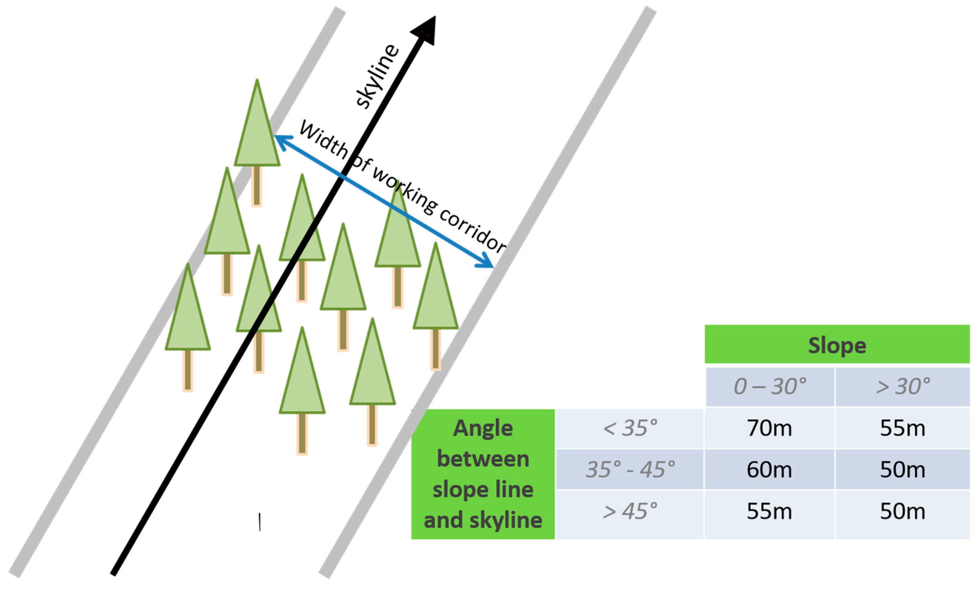
Forests 10 00687 g002
Figure 3. Width of the working corridor within a CR, depending on the slope and the angle between slope line and skyline.
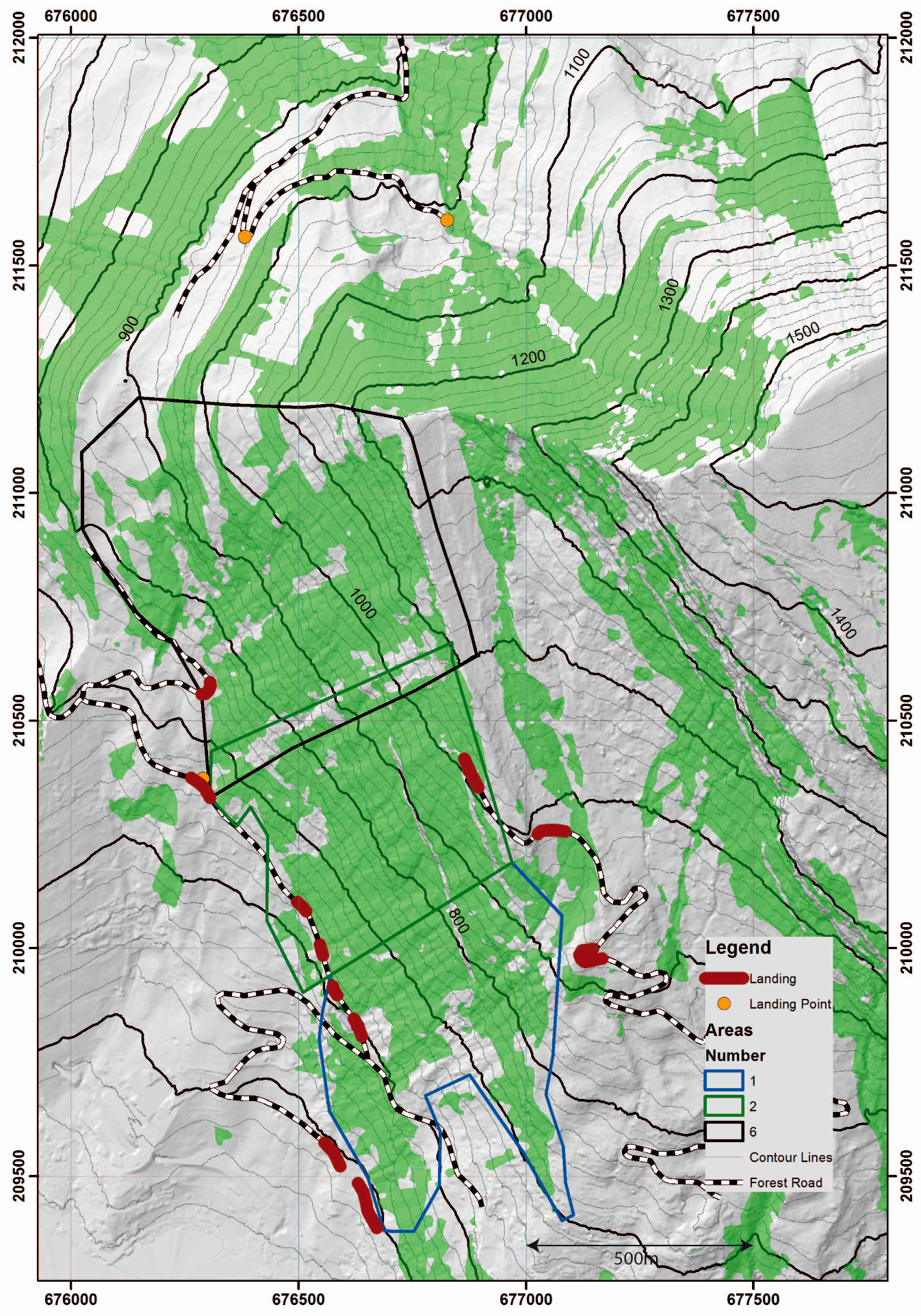
Forests 10 00687 g003
Figure 4. Rigi test areas. Here only sub-area numbers 1, 2 and 6 are displayed. Sub-areas 7, 8 and 9 are not displayed. Area 7 is composed of sub-areas of areas 6 and 2, area 8 covers areas 1 and 2, and area 9 covers the whole project area. Note that the landings and the forest road at the bottom right have a limited bearing capacity, leading to additional trans-shipment costs of 15 CHF/m3 (hillshade map © swisstopo (JA100118)).
Forests 10 00687 g004
Figure 5. Estimation of the amount of wood to harvest for some exemplary chosen numbers for the volume map.
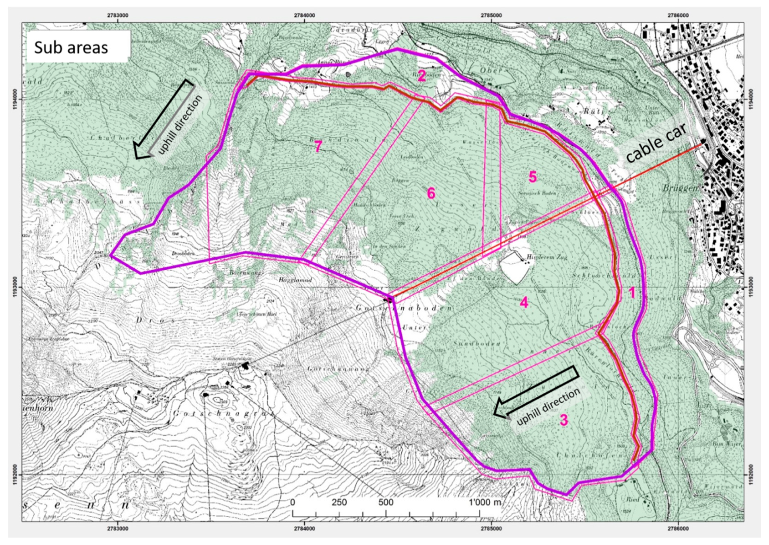
Forests 10 00687 g005
Figure 6. Sub-areas (numbered) in the Gotschna area subject to computation (topographic map © swisstopo (JA100118)).
Forests 10 00687 g006
Figure 7. CR and harvesting layouts of weighting cases 1, 3, 4, and 7 (with fH = 0.7) for area 01. The corresponding properties of those layouts can be found in Table 6.
Forests 10 00687 g007
Figure 8. Pareto-optimal solutions for Rigi, Area 01, for (a) harvesting costs and relative negative impact (RNI), with case numbers displayed; (b) downhill logging length and harvesting costs (only cases with λSL = 0); and (c) slope line length and harvesting costs (only cases with λDH = 0).
Forests 10 00687 g008
Figure 9. Harvesting layout for area 1 (Rigi) for different fH values (a: = 1, b: = 0.7, c: = 0.5) (helicopter wood extraction factor) (weighting: λSL = 0.25, λDH = 0.25, λC = 0.50). The darker green areas have a larger volume per TP. The corresponding properties of those layouts can be found in Table 6.
Forests 10 00687 g009
Figure 10. Aggregated results of the Pareto set consisting of the variants minimum harvesting costs (MIN-EK) (circle), minimum CR length in unfavorable direction (MIN-UR) (diamond) and MIX (square). In (a) the variants are characterized according to the negative net revenue and the length of CR in an unfavorable direction relative to the slope line. In (b) the variants are characterized according to the average harvest costs per cubic meter. (* objective weights applied to sub-units differ ➲ define merging rule).
Forests 10 00687 g010
Figure 11. Harvesting and CR layout for MIN-EK (minimize harvesting cost) (topographic map © swisstopo (JA100118)).
Forests 10 00687 g011
Figure 12. Harvesting and CR layout for MIX (multiobjective solution) (topographic map © swisstopo (JA100118)).
Forests 10 00687 g012
Figure 13. Harvesting and CR layout for MIN-UR (minimize length in unfavorable CR direction) (topographic map © swisstopo (JA100118)).
Forests 10 00687 g013
Table 1. Critical aisle properties for avalanches. The first column indicates that aisles steeper than 30° and longer than 60 m can cause avalanches.
SlopeLength of Aisle in Slope Line
>30°>60 m
>35°>50 m
>40°>40 m
>45°>30 m
Table 2. Penalty value for the angle of deviation of the cable roads (CR) direction from the slope line. (L: length of the CR within the corresponding angle of deviation).
Angle (α) of Deviation of the Yarding Direction from Slope LinePenalty Values
RigiGotschna
0–10°L × 0.5L
10–25°0L
25–35°00
35–45°L × 0.5L
45–90°L × 2L
Table 3. Parameters of the harvesting techniques. (MSK: short distance yarder, KSK: long distance yarder).
Harvesting TechniqueParameterUnitValues (Gotschna)Values (Rigi)
Cable yarderMinimum length (diagonal distance) (all)m100100
Maximum length (diagonal distance) (MSK/KSK)m600/8001000/--
average diagonal distance (used for calibration)m500600
Width of working corridorm60dependent on slope
Minimum ground clearance (load path)m86
Design payload (carriage and load)kN2525
Range of values for favorable deviation from slope line°25–3510–35
Installation cost (MSK/KSK) (used for calibration)CHF200/800200/800
Harvesting cost: felling, processing and yarding (MSK/KSK) (used for calibration)CHF/m372/87100/--
WinchMaximum skidding distance uphillm6060
Maximum skidding distance downhillm050
Harvesting cost: felling, processing and skiddingCHF/m34545
HelicopterHarvesting cost: felling, processing and loggingCHF/m3135150
AllAverage revenue for woodCHF/m36555
Table 4. Size and properties of the variables of the test areas. The variables have the following meaning: xic: number of combinations to harvest a timber parcel (TP) (clustered with number of clusters = 3) yk: number of CR sections, tlm: number of landings, xiH: number of TPs.
Number of Variables & Variable TypeSize (ha)
xic (nc = 3)yktlmxiH
Areacont.integercont.cont.
Rigi16430487183272228
27664444983292430
610,027259448441545
79993471961394540
812,028742892477048
921,922953192905391
Gotschna110,7816923373156135
293505716465149734
315,76314,552220306669
416,02114,849266300968
513,2018967222151534
611,18514,807138267060
720,93514,125234256958
Table 5. Key values for different objective weighting alternatives (Rigi, Sub-area 1).
Weight
CaseCostSlope LineDownhill LoggingNet Revenue (CHF)Harvesting Cost (CHF/m3)Slope Line Penalty Value (m)Length DH Logging (m)
11.0000−39,04372.516803900
20.7500.25−41,68173.417802630
30.750.250−40,10472.910853840
40.500.250.25−43,77674.18902840
50.500.500−46,69775.06803260
60.5000.50−46,89275.117001420
70.250.250.50−62,05979.95201560
80.250.500.25−62,04879.93752050
90.250.750−65,86081.12802670
100.2500.75−68,67482.0197580
110.020.240.73−168,011113.900
120.020.490.49−168,011113.900
130.020.730.24−168,011113.900
140.020.980.00−137,051104.001090
150.020.000.98−73,05583.520250
Table 6. CR and harvesting layouts properties of weighting cases 1, 3, 4, and 7. The corresponding visualizations can be found in Figure 7 and Figure 9. A. (H, W): Alternative helicopter or winch.
Case NumberfHNo. of TPs Harvested byTotal Length of CRs (m)Volume Harvested by (m3)
A. (H, W)YarderA. (H, W)YarderTotal
10.710551675531018928453034
30.711171613451025727483005
4111171613507037927363115
0.712091521386035326112964
0.51837893190076315902352
70.712911439385045224692921
Table 7. Computation time for solving the optimization problem with GUROBI [seconds] (n.s.: not solved within 2 days, n.c.: not calculated). Area numbers with an “a” (e.g. 1a, 2a) indicate that the harvesting volume for helicopter logging is less than for cable logging per parcel (fH = 1/3, basis: fH = 1/2).
WeightArea Number [Rigi] & Number of TPs
CostSlope LineDownhill11a22a66a77a88a99a
272227222924292444154415394539454770477090539053
1.000012612.9760687.392.24.6n.s.4263n.s.7108n.s.n.s.
0.7500.254668.716 35921679.02.8n.c.4441n.c.9535n.c.n.c.
0.750.2501875.5142949.617.08.0n.c.743n.c.5603n.c.n.c.
0.500.250.2560.81.1213613.017.11.8n.c.54.3n.c.1989n.c.n.c.
0.500.50021.90.61206.85.30.5n.c.7.0n.c.401n.c.n.c.
0.5000.501071.248 75112656.81.5n.c.579n.c.7993n.c.n.c.
0.250.250.5049.60.29091.45.50.4n.c.0.4n.c.3.6n.c.n.c.
0.250.500.2511.70.475.10.91.50.2n.c.0.4n.c.1.8n.c.n.c.
0.250.7501.40.94.21.20.81.0n.c.0.4n.c.4.4n.c.n.c.
0.2500.756.20.61411.02.40.4n.c.0.3n.c.0.6n.c.n.c.
0.010.250.740.40.20.50.30.20.4n.c.0.2n.c.0.3n.c.n.c.
0.010.500.500.80.20.20.60.20.2n.c.0.2n.c.0.3n.c.n.c.
0.010.740.250.30.20.30.20.20.2n.c.0.2n.c.0.3n.c.n.c.
0.010.9900.30.20.70.90.20.2n.c.0.3n.c.0.4n.c.n.c.
0.0100.991.40.36.90.20.20.2n.c.0.3n.c.0.4n.c.n.c.
Table 8. Characteristic values of the CR layouts calculated with different weights λC and λSL. “L unfavorable” quantifies the CR length in the unfavorable direction.
VariantMIN-EKMIN-URMIX
Net revenue (kCHF)−596−1790−828
L unfavorable (km)6.8150.0152.605
λC100.21
λSL010.79
Share cable Yarder (%)88.233.875.6
Share helicopter (%)11.265.223.7
Share winch (%)0.610.7
Table 9. CR and harvesting layouts properties of tested areas in Gotschna. The corresponding visualizations can be found in Figure 11, Figure 12 and Figure 13.
No. of TPs harvested byVolume Harvested by (m3)
CaseAlternativeYarderAlternativeYarderTotal
MIX10,4815406923532,47641,711
MIN-EK96236264421837,49341,711
MIN-UR13,175271225,19916,51241,711
Table 10. Properties and computation times (minutes) for the sub-areas in the Gotschna area.
Sub-Area1234567
No. of TPs1561149730663009151526702569
No. of potential CRs10,781935015,76316,02113,20111,18520,935
No. of NISE81055554
comp. time (min)5277230491019

