Comparison of Three Algorithms to Estimate Tree Stem Diameter from Terrestrial Laser Scanner Data


 , and
, and
Abstract
:1. Introduction
2. Benchmarked Algorithms for Stem Diameter Estimations
2.1. STEP Algorithm
2.2. Cylinder Fitting Algorithm
2.3. SimpleTree
3. Materials and Methods
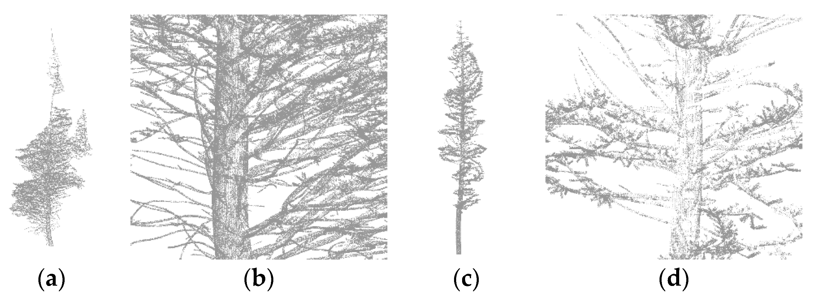
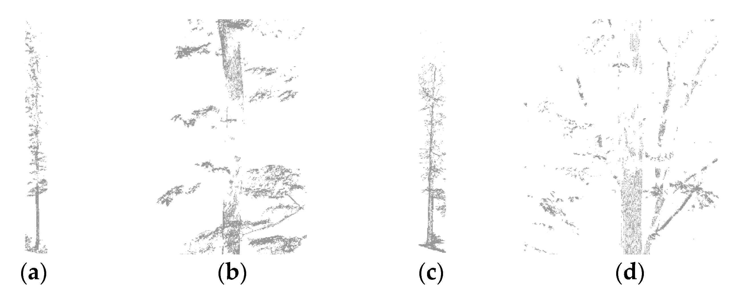
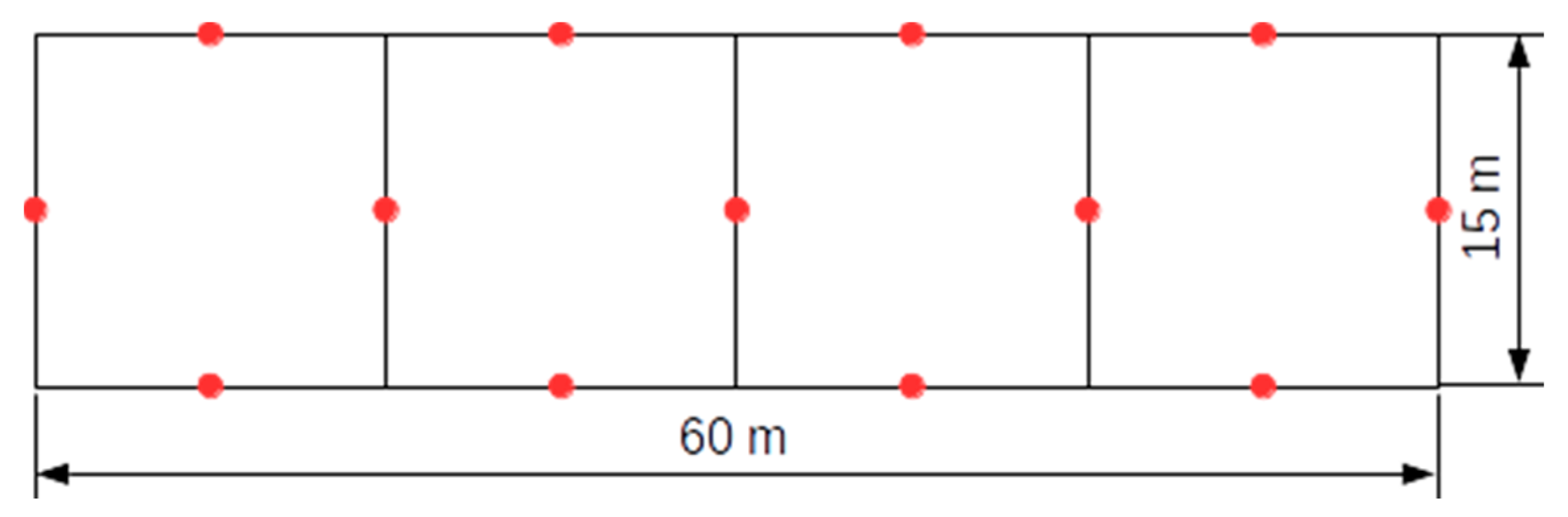
3.1. Test Sites and Data Sets
3.1.1. Newfoundland Dataset
3.1.2. Phalsbourg Data Set
3.1.3. Bas Saint-Laurent Dataset
3.2. Comparison
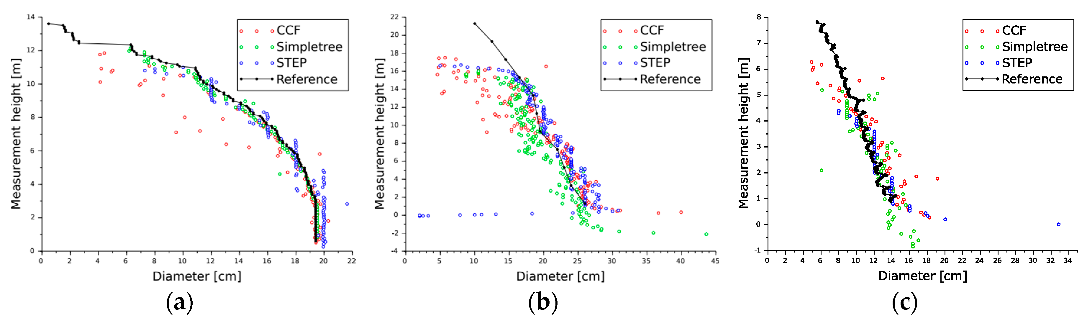
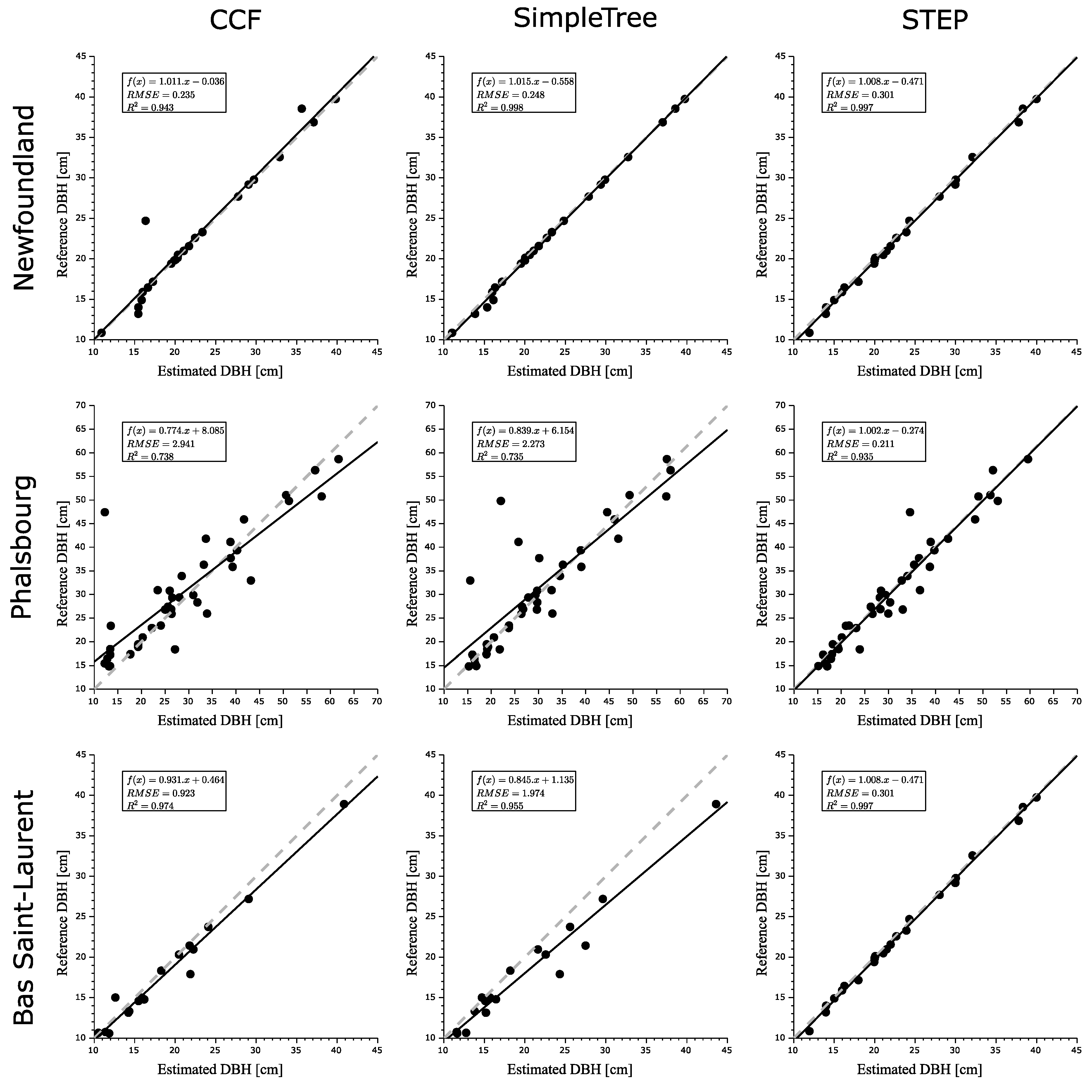
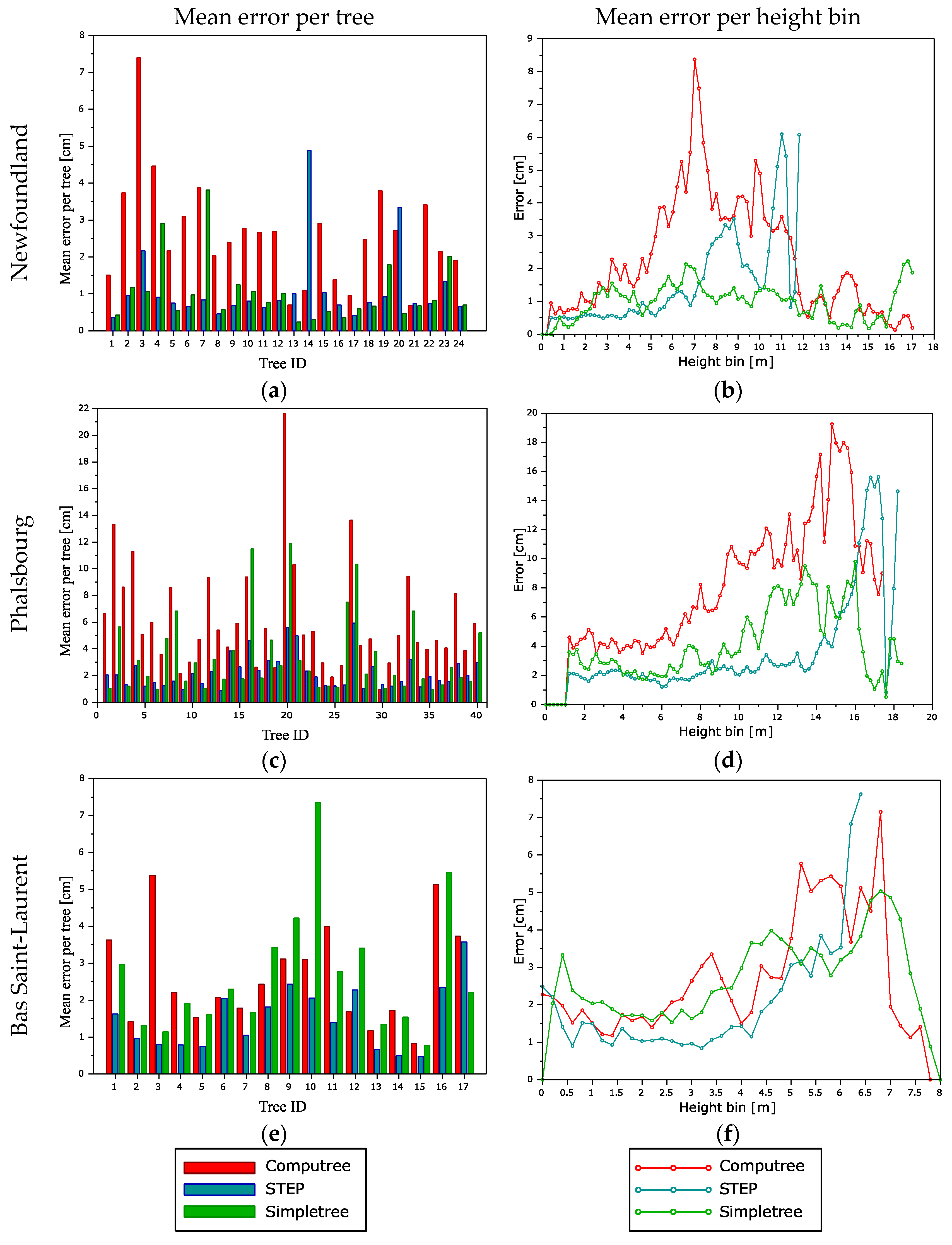
4. Results
5. Discussion
6. Conclusions
Author Contributions
Funding
Acknowledgments
Conflicts of Interest
References
- Feldpausch, T.R.; Banin, L.; Phillips, O.; Baker, T.R.; Lewis, S.L.; Quesada, C.A.; Affum-Baffoe, K.; Arets, E.J.M.M.; Berry, N.J.; Bird, M.; et al. Height-diameter allometry of tropical forest trees. Biogeosciences 2011, 8, 1081–1106. [Google Scholar] [CrossRef] [Green Version]
- Fortin, M.; Schneider, R.; Saucier, J.-P. Volume and Error Variance Estimation Using Integrated Stem Taper Models. For. Sci. 2012, 59, 345–358. [Google Scholar] [CrossRef]
- Wulder, M.A.; White, J.C.; Fournier, R.A.; Luther, J.E.; Magnussen, S. Spatially Explicit Large Area Biomass Estimation: Three Approaches Using Forest Inventory and Remotely Sensed Imagery in a GIS. Sensors 2008, 8, 529–560. [Google Scholar] [CrossRef] [PubMed] [Green Version]
- Black, K.; Reidy, B.; Bolger, T.; Tobin, B.; Osborne, B.; Nieuwenhuis, M. Assessment of allometric algorithms for estimating leaf biomass, leaf area index and litter fall in different-aged Sitka spruce forests. Forestry 2006, 79, 453–465. [Google Scholar]
- Köhl, M.; Magnussen, S.; Marchetti, M. Sampling Methods, Remote Sensing and GIS Multiresource Forest Inventory; Springer Science & Business Media: Berlin, Germany, 2006. [Google Scholar]
- van Laar, A.; Akca, A. Forest Mensuration; Springer Science & Business Media: Berlin, Germany, 2007. [Google Scholar]
- Avery, T.E.; Burkhart, H.E. Forest Measurements; McGraw-Hill: New York, NY, USA, 2001. [Google Scholar]
- Dassot, M.; Colin, A.; Santenoise, P.; Fournier, M.; Constant, T. Terrestrial laser scanning for measuring the solid wood volume, including branches, of adult standing trees in the forest environment. Comput. Electron. Agric. 2012, 89, 86–93. [Google Scholar] [CrossRef]
- Dassot, M.; Constant, T.; Fournier, M. The use of terrestrial LiDAR technology in forest science: Application fields, benefits and challenges. Ann. For. Sci. 2011, 68, 959–974. [Google Scholar] [CrossRef]
- Vosselman, G.; Maas, H.-G. Airborne and Terrestrial Laser Scanning; CRC Press: Boca Raton, FL, USA, 2010; p. 318. [Google Scholar]
- Bouvier, M.; Durrieu, S.; Fournier, R.; Saint-Geours, N.; Vincent, G.; Guyon, D.; Grau, E.; Hérault, B. Influence of sampling design parameters on biomass predictions derived from airborne lidar data. In Proceedings of the SilviLaser 2015, La Grande Motte, France, 28–30 September 2015; pp. 137–139. [Google Scholar]
- Falkowski, M.J.; Smith, A.M.; Hudak, A.T.; E Gessler, P.; A Vierling, L.; Crookston, N.L. Automated estimation of individual conifer tree height and crown diameter via two-dimensional spatial wavelet analysis of lidar data. Can. J. Remote Sens. 2006, 32, 153–161. [Google Scholar] [CrossRef] [Green Version]
- Næsset, E. Predicting forest stand characteristics with airborne scanning laser using a practical two-stage procedure and field data. Remote Sens. Environ. 2002, 80, 88–99. [Google Scholar] [CrossRef]
- Vepakomma, U.; St-Onge, B.; Kneeshaw, D. Spatially explicit characterization of boreal forest gap dynamics using multi-temporal lidar data. Remote Sens. Environ. 2008, 112, 2326–2340. [Google Scholar] [CrossRef]
- Liang, X.; Kankare, V.; Hyyppä, J.; Wang, Y.; Kukko, A.; Haggrén, H.; Yu, X.; Kaartinen, H.; Jaakkola, A.; Guan, F.; et al. Terrestrial laser scanning in forest inventories. ISPRS J. Photogramm. Remote Sens. 2016, 115, 63–77. [Google Scholar] [CrossRef]
- Metz, J.; Seidel, D.; Schall, P.; Scheffer, D.; Schulze, E.-D.; Ammer, C. Crown modeling by terrestrial laser scanning as an approach to assess the effect of aboveground intra-and interspecific competition on tree growth. For. Ecol. Manag. 2013, 310, 275–288. [Google Scholar] [CrossRef]
- Olivier, M.-D.; Robert, S.; Fournier, R.A. Response of sugar maple (Acer saccharum, Marsh.) tree crown structure to competition in pure versus mixed stands. For. Ecol. Manag. 2016, 374, 20–32. [Google Scholar] [CrossRef]
- Durrieu, S.; Allouis, T.; Fournier, R.; Véga, C.; Albrech, L. Spatial quantification of vegetation density from terrestrial laser scanner data for characterization of 3D forest structure at plot level. In Proceedings of the SilviLaser 2008, Edinburgh, UK, 17–19 September 2008; pp. 325–334. [Google Scholar]
- Béland, M.; Widlowski, J.-L.; Fournier, R.A.; Côté, J.-F.; Verstraete, M.M. Estimating leaf area distribution in savanna trees from terrestrial LiDAR measurements. Agric. For. Meteorol. 2011, 151, 1252–1266. [Google Scholar] [CrossRef]
- Hosoi, F.; Nakai, Y.; Omasa, K. Voxel tree modeling for estimating leaf area density and woody material volume using 3-D LIDAR data. ISPRS Ann. Photogramm. Remote Sens. Spat. Inf. Sci. 2013, 5, 115–120. [Google Scholar] [CrossRef]
- Côté, J.-F.; Fournier, R.A.; Egli, R. An architectural model of trees to estimate forest structural attributes using terrestrial LiDAR. Environ. Model. Softw. 2011, 26, 761–777. [Google Scholar] [CrossRef]
- Côté, J.-F.; Fournier, R.A.; Frazer, G.W.; Niemann, K.O. A fine-scale architectural model of trees to enhance LiDAR-derived measurements of forest canopy structure. Agric. For. Meteorol. 2012, 166, 72–85. [Google Scholar] [CrossRef]
- Blanchette, D.; Fournier, R.A.; Luther, J.E.; Côté, J.-F. Predicting wood fiber attributes using local-scale metrics from terrestrial LiDAR data: A case study of Newfoundland conifer species. For. Ecol. Manag. 2015, 347, 116–129. [Google Scholar] [CrossRef]
- Othmani, A.; Piboule, A.; Krebs, M.; Stolz, C. Towards automated and operational forest inventories with T-Lidar. In Proceedings of the SilviLaser 2011, Hobart, Australia, 16–20 October 2011; pp. 1–9. [Google Scholar]
- Kuusk, A.; Lang, M.; Märdla, S.; Pisek, J. Tree stems from terrestrial laser scanner measurements. For. Stud. 2015, 63, 44–55. [Google Scholar] [CrossRef] [Green Version]
- Brunner, A.; Gizachew, B. Rapid detection of stand density, tree positions, and tree diameter with a 2D terrestrial laser scanner. Eur. J. For. Res. 2014, 133, 819–831. [Google Scholar] [CrossRef]
- Henning, J.G.; Radtke, P.J. Detailed stem measurements of standing trees from ground-based scanning lidar. For. Sci. 2006, 52, 67–80. [Google Scholar]
- Bienert, A.; Scheller, S.; Keane, E.; Mullooly, G.; Mohan, F. Application of Terrestrial Laser Scanners For The Determination Of Forest Inventory Parameters. Int. Arch. Photogramm. Remote Sens. Spat. Inf. Sci. 2006, 36, 5. [Google Scholar]
- Schilling, A.; Schmidt, A.; Maas, H.-G. Automatic Tree Detection and Diameter Estimation in Terrestrial Laser Scanner Point Clouds. In Proceedings of the 16th Computer Vision Winter Workshop, Mitterberg, Austria, 2–4 February 2011; pp. 75–83. [Google Scholar]
- Lindberg, E.; Holmgren, J.; Olofsson, K.; Olsson, H. Estimation of stem attributes using a combination of terrestrial and airborne laser scanning. Eur. J. For. Res. 2012, 131, 1917–1931. [Google Scholar] [CrossRef] [Green Version]
- Olofsson, K.; Holmgren, J.; Olsson, H. Tree Stem and Height Measurements using Terrestrial Laser Scanning and the RANSAC Algorithm. Remote Sens. 2014, 6, 4323–4344. [Google Scholar] [CrossRef] [Green Version]
- Király, G.; Brolly, G. Modelling single trees from terrestrial laser scanning data in a forest reserve. Photogramm. J. Finl. 2008, 21, 37–50. [Google Scholar]
- Aschoff, T.; Spiecker, H. Algorithms for the automatic detection of trees in laser scanner data. Int. Arch. Photogramm. Remote Sens. Spat. Inf. Sci. 2004, 36, W2. [Google Scholar]
- Pál, I. Measurements of Forest Inventory Parameters on Terrestrial Laser Scanning Data Using Digital Geometry and Topology. Int. Arch. Photogramm. Remote Sens. Spat. Inf. Sci. 2008, 37, 373–380. [Google Scholar]
- Belton, D.; Moncrieff, S.; Chapman, J. Processing tree point clouds using Gaussian Mixture Models. In Proceedings of the ISPRS annals of the photogrammetry, remote sensing and spatial information sciences, Antalya, Turkey, 1–13 November 2013. [Google Scholar]
- Aiteanu, F.; Klein, R. Hybrid tree reconstruction from inhomogeneous point clouds. Vis. Comput. 2014, 30, 763–771. [Google Scholar] [CrossRef]
- Åkerblom, M.; Raumonen, P.; Kaasalainen, M.; Casella, E.; Baghdadi, N.; Thenkabail, P.S. Analysis of Geometric Primitives in Quantitative Structure Models of Tree Stems. Remote Sens. 2015, 7, 4581–4603. [Google Scholar] [Green Version]
- Simonse, M.; Aschoff, T.; Spiecker, H.; Thies, M. Automatic determination of forest inventory parameters using terrestrial laser scanning. In Proceedings of the ScandLaser Scientific Workshop on Airborne Laser Scanning of Forests, Umeå, Sweden, 3–4 September 2003; Volume 2003, pp. 252–258. [Google Scholar]
- Pfeifer, N.; Winterhalder, D.; Gorte, B.G.H. Three-dimensional reconstruction of stems for assessment of taper, sweep and lean based on laser scanning of standing trees. Scand. J. For. Res. 2004, 19, 571–581. [Google Scholar]
- Hackenberg, J.; Morhart, C.; Sheppard, J.; Spiecker, H.; Disney, M. Highly Accurate Tree Models Derived from Terrestrial Laser Scan Data: A Method Description. Forests 2014, 5, 1069–1105. [Google Scholar] [CrossRef] [Green Version]
- Wezyk, P.; Kozioł, K.; Glista, M.; Pierzchalski, M. Terrestrial laser scanning versus traditional forest inventory first results from the polish forests. In Proceedings of the ISPRS Workshop on Laser Scanning 2007 and SilviLaser 2007, Espoo, Finland, 12–14 September 2007; Volume 36, pp. 424–429. [Google Scholar]
- Yan, D.; Wintz, J.; Mourrain, B.; Wang, W.; Bourdon, F.; Godin, C. Efficient and robust tree model reconstruction from laser scanned data points. In Proceedings of the 11th IEEE International conference on Computer-Aided Design and Computer Graphics 2009, Huangshan, China, 19–21 August 2009; pp. 572–576. [Google Scholar]
- Moskal, L.M.; Zheng, G. Retrieving forest inventory variables with terrestrial laser scanning (TLS) in urban heterogeneous forest. Remote Sens. 2012, 4, 1–20. [Google Scholar] [CrossRef]
- Pfeifer, N.; Winterhalder, D. Modelling of tree cross sections from terrestrial laser scanning data with free-form curves. Int. Arch. Photogramm. Remote Sens. Spat. Inf. Sci. 2004, 36, W2. [Google Scholar]
- Liang, X.; Litkey, P.; Hyyppa, J.; Kaartinen, H.; Vastaranta, M.; Holopainen, M. Automatic Stem Mapping Using Single-Scan Terrestrial Laser Scanning. IEEE Trans. Geosci. Remote Sens. 2012, 50, 661–670. [Google Scholar] [CrossRef]
- Kankare, V.; Liang, X.; Yu, X.; Hyyppa, J.; Holopainen, M. Automated Stem Curve Measurement Using Terrestrial Laser Scanning. IEEE Trans. Geosci. Remote Sens. 2014, 52, 1739–1748. [Google Scholar]
- Kelbe, D.; Romanczyk, P.; Van Aardt, J.; Cawse-Nicholson, K. Reconstruction of 3D tree stem models from low-cost terrestrial laser scanner data. In Laser Radar Technology and Applications XVIII; International Society for Optics and Photonics: Bellingham, WA, USA, 2013; Volume 8731, p. 873106. [Google Scholar]
- McDaniel, M.W.; Nishihata, T.; Brooks, C.A.; Salesses, P.; Iagnemma, K. Terrain classification and identification of tree stems using ground-based LiDAR. J. Field Robot. 2012, 29, 891–910. [Google Scholar] [CrossRef]
- Kelbe, D.; Romanczyk, P. Automatic extraction of tree stem models from single terrestrial lidar scans in structurally heterogeneous forest environments. In Proceedings of the 12th International Conference on LiDAR Applications for Assessing Forest Ecosystems 2012, Vancouver, BC, Canada, 16–19 September 2012; pp. 1–8. [Google Scholar]
- Hildebrandt, R.; Iost, A. From points to numbers: A database-driven approach to convert terrestrial LiDAR point clouds to tree volumes. Eur. J. For. Res. 2012, 131, 1857–1867. [Google Scholar] [CrossRef]
- Aschoff, T.; Thies, M.; Spiecker, H. Describing forest stands using terrestrial laser-scanning. Int. Arch. Photogramm. Remote Sens. Spat. Inf. Sci. 2004, 35, 237–241. [Google Scholar]
- Huang, H.; Li, Z.; Gong, P.; Cheng, X.; Clinton, N.; Cao, C.; Ni, W.; Wang, L. Automated Methods for Measuring DBH and Tree Heights with a Commercial Scanning Lidar. Photogramm. Eng. Remote Sens. 2011, 77, 219–227. [Google Scholar] [CrossRef]
- Xi, Z.; Hopkinson, C.; Chasmer, L. Automating Plot-Level Stem Analysis from Terrestrial Laser Scanning. Forests 2016, 7, 252. [Google Scholar] [CrossRef]
- Ravaglia, J.; Bac, A.; Fournier, R.A. Extraction of tubular shapes from dense point clouds and application to tree reconstruction from laser scanned data. Comput. Graph. 2017, 66, 23–33. [Google Scholar] [CrossRef]
- Côté, J.-F.; Fournier, R.A.; Luther, J.E. Validation of L-Architect model for balsam fir and black spruce trees with structural measurements. Can. J. Remote Sens. 2013, 39, S41–S59. [Google Scholar] [CrossRef]
- Raumonen, P.; Kaasalainen, M.; Akerblom, M.; Kaasalainen, S.; Kaartinen, H.; Vastaranta, M.; Holopainen, M.; Disney, M.; Lewis, P. Fast Automatic Precision Tree Models from Terrestrial Laser Scanner Data. Remote Sens. 2013, 5, 491–520. [Google Scholar] [CrossRef] [Green Version]
- Raumonen, P.; Casella, E.; Calders, K.; Murphy, S.; Åkerbloma, M.; Kaasalainen, M. Massive-Scale Tree Modelling from TLS Data. ISPRS Ann. Photogramm. Remote Sens. Spat. Inf. Sci. 2015, II-3/W4, 189–196. [Google Scholar] [CrossRef]
- Hackenberg, J.; Wassenberg, M.; Spiecker, H.; Sun, D. Non Destructive Method for Biomass Prediction Combining TLS Derived Tree Volume and Wood Density. Forests 2015, 6, 1274–1300. [Google Scholar] [CrossRef]
- Hackenberg, J.; Spiecker, H.; Calders, K.; Disney, M.; Raumonen, P. SimpleTree—An Efficient Open Source Tool to Build Tree Models from TLS Clouds. Forests 2015, 6, 4245–4294. [Google Scholar] [CrossRef]
- Amanatides, J.; Woo, A. A Fast Voxel Traversal Algorithm for Ray Tracing; Eurographics: Montreal, QC, Canada, 1987; Volume 87, pp. 3–10. [Google Scholar]
- Kass, M.; Witkin, A.; Terzopoulos, D. Snakes: Active contour models. Int. J. Comput. Vis. 1988, 1, 321–331. [Google Scholar] [CrossRef]
- Ravaglia, J.; Bac, A.; Fournier, R.A. Anisotropic Octrees: A Tool for Fast Normals Estimation on Unorganized Point Clouds. In Proceedings of the Winter School of Computer Graphics (WSCG) 2017, Plzen, Czech Republic, 29 May–2 June 2017. [Google Scholar]
- Pfeifer, N.; Gorte, B.; Winterhalder, D. Automatic Reconstruction of Single Trees From Terrestrial Laser Scanner Data. In Proceedings of the 20th ISPRS Congress, Istanbul, Turkey, 12–23 July 2004; pp. 114–119. [Google Scholar]
- Pôle Recherche Développement Innovation, Office National des Forêts. Computree Official Website. 2019. Available online: http://computree.onf.fr/?lang=en (accessed on 5 August 2017).
- Pharr, M.; Jakob, W.; Humphreys, G. Physically Based Rendering: From Theory to Implementation; Morgan Kaufmann: Burlington, MA, USA, 2016. [Google Scholar]
- Saucier, J.-P.; Grondin, P.; Robitaille, A.; Bergeron, J.-F. Zone de Végétation des Domaines Bioclimatiques du Québec; Ministère des Ressources Naturelles, Direction des Inventaires Forestiers: Quebec, QC, Canada, 2001.
- Pitkänen, T.P.; Raumonen, P.; Kangas, A. Measuring stem diameters with TLS in boreal forests by complementary fitting procedure. ISPRS J. Photogramm. Remote Sens. 2019, 147, 294–306. [Google Scholar] [CrossRef]
- Calders, K.; Newnham, G.; Burt, A.; Murphy, S.; Raumonen, P.; Herold, M.; Culvenor, D.; Avitabile, V.; Disney, M.; Armston, J.; et al. Nondestructive estimates of above-ground biomass using terrestrial laser scanning. Methods Ecol. Evol. 2015, 6, 198–208. [Google Scholar] [CrossRef]
- Wang, P.; Li, R.; Bu, G.; Zhao, R. Automated low-cost terrestrial laser scanner for measuring diameters at breast height and heights of plantation trees. PLoS ONE 2019, 14, e0209888. [Google Scholar] [CrossRef]
- Zhang, W.; Wan, P.; Wang, T.; Cai, S.; Chen, Y.; Jin, X.; Yan, G. A Novel Approach for the Detection of Standing Tree Stems from Plot-Level Terrestrial Laser Scanning Data. Remote Sens. 2019, 11, 211. [Google Scholar] [CrossRef]
- Kunz, M.; Hess, C.; Raumonen, P.; Bienert, A.; Hackenberg, J.; Maas, H.-G.; Härdtle, W.; Fichtner, A.; Oheimb, G. Comparison of wood volume estimates of young trees from terrestrial laser scan data. iForest Biogeosci. For. 2017, 10, 451–458. [Google Scholar] [CrossRef] [Green Version]
- Gonzalez de Tanago, J.; Lau, A.; Bartholomeus, H.; Herold, M.; Avitabile, V.; Raumonen, P.; Martius, C.; Goodman, R.C.; Disney, M.; Manuri, S.; et al. Estimation of above-ground biomass of large tropical trees with terrestrial LiDAR. Methods Ecol. Evol. 2018, 9, 223–234. [Google Scholar] [CrossRef]
- Maas, H.-G.; Bienert, A.; Scheller, S.; Keane, E. Automatic forest inventory parameter determination from terrestrial laser scanner data. Int. J. Remote Sens. 2008, 29, 1579–1593. [Google Scholar] [CrossRef]
- Leblanc, S.; Fournier, R. Hemispherical photography simulations with an architectural model to assess retrieval of leaf area index. Agric. For. Meteorol. 2014, 194, 64–76. [Google Scholar] [CrossRef]
- Côté, J.-F.; Fournier, R.A.; Luther, J.E.; Van Lier, O.R. Fine-scale three-dimensional modeling of boreal forest plots to improve forest characterization with remote sensing. Remote Sens. Environ. 2018, 219, 99–114. [Google Scholar] [CrossRef]
- Rusu, R.B.; Cousins, S. 3D is here: Point Cloud Library (PCL). In Proceedings of the IEEE International Conference on Robotics and Automation, Shanghai, China, 9–13 May 2011. [Google Scholar]
- Boulch, A.; Marlet, R. Deep Learning for Robust Normal Estimation in Unstructured Point Clouds. Comput. Graph. Forum 2016, 35, 281–290. [Google Scholar] [CrossRef] [Green Version]
- Brodu, N.; Lague, D. 3D terrestrial lidar data classification of complex natural scenes using a multi-scale dimensionality criterion: Applications in geomorphology. ISPRS J. Photogramm. Remote Sens. 2012, 68, 121–134. [Google Scholar] [CrossRef] [Green Version]
- Martin-Ducup, O.; Schneider, R.; Fournier, R.A. Analyzing the Vertical Distribution of Crown Material in Mixed Stand Composed of Two Temperate Tree Species. Forests 2018, 9, 673. [Google Scholar] [CrossRef]


| Study Site | Newfoundland | Phalsbourg | Bas Saint-Laurent |
|---|---|---|---|
| Stand type | Coniferous | Mixed (mainly deciduous) | Coniferous |
| Tree species | Black Spruce Balsam Fir | Common beech Hornbeam | White spruce |
| Number of selected trees | 24 | 40 | 17 |
| Minimum DBH | 5.43 cm | 10 cm | 9 cm |
| Maximum DBH | 19.88 cm | 70 cm | 40 cm |
| TLS scanner | Simulated (PBRT) | Faro Focus 3D© | Faro Focus 3D A120© |
| Scanner angular resolution | 0.036° | 0.036° | 0.018° |
| Number of scans per plot | 5 | 4 | 4 |
| Reconstruction Height [m] | Algorithm | Newfoundland Site | Phalsbourg Site | Bas Saint-Laurent Site |
|---|---|---|---|---|
| Mean | CCF SimpleTree STEP | 9.35 10.22 8.80 | 11.02 11.21 10.66 | 5.95 6.37 4.88 |
| Std deviation | CCF SimpleTree STEP | 3.29 3.22 2.09 | 4.17 3.61 3.58 | 0.92 1.09 1.42 |
| Diameter Error per Tree [cm] | Algorithm | Newfoundland Site (24 Selected Trees) | Phalsbourg Site (40 Selected Trees) | Bas Saint-Laurent Site (17 Selected Trees) | |||
|---|---|---|---|---|---|---|---|
| Abs [cm] | Rel [%] | Abs [cm] | Rel [%] | Abs [cm] | Rel [%] | ||
| Minimum | CCF SimpleTree STEP | 0.69 0.24 0.37 | 5.82 1.61 2.00 | 0.96 0.95 0.93 | 5.98 3.82 3.11 | 0.83 0.77 0.47 | 18.92 8.13 4.69 |
| Global average | CCF SimpleTree STEP | 2.61 1.10 1.13 | 16.01 6.75 11.31 | 6.25 3.41 2.34 | 23.61 12.54 9.34 | 2.60 2.64 1.52 | 18.52 16.94 8.95 |
| Global Std deviation | CCF SimpleTree STEP | 3.94 2.51 2.61 | 28.03 11.26 63.68 | 7.47 5.32 3.09 | 24.27 16.59 12.88 | 3.44 2.74 1.83 | 28.12 13.95 10.57 |
| Global RMSE | CCF SimpleTree STEP | 4.72 2.74 2.84 | - - - | 9.74 6.32 3.87 | - - - | 4.31 3.80 2.38 | - - - |
| Average error at tree-level | CCF SimpleTree STEP | 2.62 1.03 1.11 | 15.78 6.55 10.40 | 6.1 3.34 2.28 | 24.71 12.72 9.76 | 2.64 2.67 1.5 | 18.92 16.85 9.31 |
| Std deviation at tree-level | CCF SimpleTree STEP | 1.44 0.85 1.01 | 6.97 4.11 19.18 | 3.96 2.88 1.25 | 11.44 7.10 4.11 | 1.35 1.72 0.87 | 12.31 5.01 4.82 |
| Average RMSE at tree-level | CCF SimpleTree STEP | 4.38 1.86 1.79 | - - - | 8.09 4.73 3.13 | - - - | 3.85 3.29 2.03 | - - - |
| Maximum | CCF SimpleTree STEP | 7.39 3.81 4.88 | 32.05 15.12 89.21 | 21.65 11.87 5.93 | 62.30 28.97 19.15 | 5.37 7.35 3.57 | 60.81 27.27 24.25 |
© 2019 by the authors. Licensee MDPI, Basel, Switzerland. This article is an open access article distributed under the terms and conditions of the Creative Commons Attribution (CC BY) license (http://creativecommons.org/licenses/by/4.0/).
Share and Cite
Ravaglia, J.; Fournier, R.A.; Bac, A.; Véga, C.; Côté, J.-F.; Piboule, A.; Rémillard, U. Comparison of Three Algorithms to Estimate Tree Stem Diameter from Terrestrial Laser Scanner Data. Forests 2019, 10, 599. https://doi.org/10.3390/f10070599
Ravaglia J, Fournier RA, Bac A, Véga C, Côté J-F, Piboule A, Rémillard U. Comparison of Three Algorithms to Estimate Tree Stem Diameter from Terrestrial Laser Scanner Data. Forests. 2019; 10(7):599. https://doi.org/10.3390/f10070599
Chicago/Turabian StyleRavaglia, Joris, Richard A. Fournier, Alexandra Bac, Cédric Véga, Jean-François Côté, Alexandre Piboule, and Ulysse Rémillard. 2019. "Comparison of Three Algorithms to Estimate Tree Stem Diameter from Terrestrial Laser Scanner Data" Forests 10, no. 7: 599. https://doi.org/10.3390/f10070599
APA StyleRavaglia, J., Fournier, R. A., Bac, A., Véga, C., Côté, J.-F., Piboule, A., & Rémillard, U. (2019). Comparison of Three Algorithms to Estimate Tree Stem Diameter from Terrestrial Laser Scanner Data. Forests, 10(7), 599. https://doi.org/10.3390/f10070599