Characterizing Diameter Distributions for Uneven-Aged Pine-Oak Mixed Forests in the Qinling Mountains of China

Abstract

Pine-oak mixed forests in the Qinling Mountains are an essential part of the ecosystem in Northwestern China. Diameter distribution models for four species groups of pine-oak mixed forests were developed using the Weibull function. Both moment and hybrid estimation approaches were used to predict the Weibull parameters. For each approach, three fitting methods (maximum likelihood estimator regression (MLER), cumulative distribution function regression (CDFR) and modified CDFR) were employed to obtain estimates for coefficients of regression equations to predict Weibull parameters. Overall results indicated that the Moment Estimation approach was better than the Hybrid approach, and that the CDFR method was superior to the MLER and modified CDFR methods. The combination of Moment Estimation and CDFR is recommended. The models constructed in this study enable the prediction of the diameter distribution of uneven-aged pine-oak mixed forests in the Qinling Mountains based on common stand-level information.

1. Introduction

As the major forest type at mid-elevation (1000–2300 m) in the Qinling Mountains, pine-oak mixed forests dominated by Pinus tabulaeformis, Pinus armandii and Quercus aliena var. acuteserrata have been considered as the cornerstone of the local ecosystem, which supports a huge variety of plants and wildlife. The pine-oak forests in the Qinling Mountains were naturally regenerated after harvesting during the 1960s and 1970s. Therefore, the pine-oak forests are mostly in the middle of a succession process. In other words, the dynamics of the stand structure is crucial in the prediction of growth and yield for such forests.

As the most direct and measurable factor, diameter is generally related to other important variables including basal area, density and volume. This makes the diameter distribution model a useful tool to provide more detailed information about the stand without additional inventory costs [1]. As a linkage between the whole stand model and the individual tree model, the diameter distribution model has been extensively explored by researchers and foresters [2,3,4].

A variety of probability density functions (PDFs) including exponential [5], log-normal [6], gamma [7], beta [8], Weibull [9] and Johnson’s S_B [10] have been applied to characterize tree diameter distribution. Among these functions, the Weibull function might be the most popular because of its flexibility in shape and simplicity of mathematical operations. It has been widely used to describe the diameter distribution of loblolly pine [11,12,13,14,15], slash pine [16,17], black spruce [18], Scots pine [19], European beech [1], longleaf pine [20], Austrian black pine [21] and cork oak [22], as well as mixed species [23,24,25,26].

The PDF parameters of the Weibull function are usually predicted by the parameter prediction or recovery approach [27]. In the parameter prediction approach, parameters are predicted from stand variables by use of regression equations. The parameter recovery approach involves predicting diameter moments or percentiles from stand variables, and then using these values to recover the PDF parameters.

Coefficients of the regression equations were generally estimated by ordinary least squares (OLS) or seemingly unrelated regression (SUR). Cao [28] introduced the maximum likelihood estimator regression (MLER) and also the cumulative distribution function regression (CDFR), both of which turned out to perform better than the previous methods. The Modified CDFR method, obtained by computing CDF with diameter class information, was found by Poudel and Cao [15] to produce better results than the CDFR method.

The diameter distribution of pine-oak forests varies depending on succession stages, site conditions, forest types, and silvicultural treatments. This makes the prediction of stand structure for pine-oak forests difficult. Even though diameter distributions play an important role in effective forest management and planning, diameter distribution models for pine-oak mixed forests in the Qinling Mountains are still lacking. The objectives of this study were to: (1) develop diameter distribution models for uneven-aged pine-oak mixed forests in the Qinling Mountains of China; (2) evaluate two approaches to predict the parameters of the Weibull function for pine-oak forest diameter distributions; and (3) evaluate three methods of model fitting for each of the above prediction approaches.

2. Data

The data used in this study were collected between 2013 and 2014 from three forest regions in the Qinling Mountains of China: Xinjiashan (E 106°26′–106°38′, N 34°10′–34°20′), Huoditang (E 108°21′–108°29′, N 33°18′–33°28′) and Xunyangba (E 103°58′–109°48′, N 32°29′–33°13′). Plots of size 0.04 ha (20 m × 20 m) were randomly established where all trees with a minimum diameter at breast height (dbh) of 5 cm were tallied. A total of 8490 trees were measured in 152 plots. Figure 1 presents the locations of the sampling plots.

The stands consisted of three primary tree species, Pinus tabulaeformis Carr., Pinus armandii Franch., and Quercus aliena var. acuteserrata Maxim., as well as other species including Toxicodendron vernicifluum (Stokes) F.A.Barkl., Acer davidii Franch. and Betula albo-sinensis Burk. Even though the total amount of trees of all the miscellaneous species formed a considerable proportion in the stands, the number for each of them was small (usually less than 10% in a stand). Hence, all the miscellaneous species were pooled into one species group in this study. Twenty-two of the plots were dominated by P. tabulaeformis, 26 by P. armandii, and 55 by Q. aliena var. acuteserrata. The remaining 49 plots were dominated by the miscellaneous species. For the sake of simplification, P. tabulaeformis, P. armandii, Q. aliena var. acuteserrata and the miscellaneous species were specified as species group 1, 2, 3 and 4, respectively. The plots were categorized based on the proportion of stand basal area for each species group. Figure 2 shows the diameter distribution of each species group for all plots.

The two-fold cross-validation scheme [29] was applied in this study by dividing the data into two groups of 76 plots each (

Table 1. Means (and standard deviations) of stand attributes for each species, by group.

Group	Attribute	Tree Species a
		1	2	3	4	All
1 (76 plots)	Tree diameter (cm) b	20.4 (7.9)	17.7 (5.3)	21.4 (13.5)	13.2 (3.1)	17.2 (3.3)
	Basal area (m2/ha)	4.4 (7.2)	6.0 (5.8)	9.8 (11.1)	9.0 (6.3)	29.2 (8.4)
	Number of trees/ha	109 (156)	287 (325)	307 (336)	650 (449)	1353 (548)
	Dominant height (m) c					13.6 (2.7)
2 (76 plots)	Tree diameter (cm)	22.5 (9.4)	19.0 (8.9)	17.4 (8.9)	13.4 (4.2)	17.3 (3.4)
	Basal area (m2/ha)	5.4 (8.1)	6.4 (7.4)	10.0 (9.1)	9.7 (7.7)	31.4 (7.6)
	Number of trees/ha	130 (184)	234 (331)	420 (348)	655 (458)	1439 (541)
	Dominant height (m)					13.9 (2.5)

^a Tree species 1 = Pinus tabulaeformis Carr.; 2 = Pinus armandii Franch.; 3 = Quercus aliena var. acuteserrata Maxim.; 4 = other species; all = all tree species. ^b Tree diameter indicates quadratic mean diameter. ^c Dominant height is the average height of the dominant and codominant trees.

). Model parameters estimated from data of one group were used to predict for the other group. Evaluation statistics were then calculated based on predictions from both groups.

3. Methods

The Weibull PDF, used to characterize diameter distributions, has the following form:

$$f\left(x\right)=\left(\frac{c}{b}\right){\left(\frac{x-a}{b}\right)}^{c-1}\exp \left[-{\left(\frac{x-a}{b}\right)}^c\right];x\ge a,b>0,c>0$$

(1)

where x is tree dbh; a, b, and c are, respectively, the location, scale, and shape parameters of the Weibull distribution.

In this study, parameter a was set at 5 cm, which was the minimum diameter of all measured trees.

Because the pine-oak forests are uneven-aged, commonly used stand variables such as age and site index were not used in this study. The general model for regression equations to predict the Weibull parameters and moments was as follows:

$$y_s=f\left(D_{q_s},B{A}_s,N_s,D_q,BA,N,H_d,RS,\frac{D_{q_s}}{D_q},\frac{B{A}_s}{BA},\frac{N_s}{N}\right)$$

(2)

where y_s is either a specific Weibull parameter or diameter variance for species s; D_q, BA, N are stand quadratic mean diameter, basal area, and number of trees per ha, respectively; H_d is stand dominant height; and RS is relative spacing, $\left(\sqrt{10,000/N}\right)/H_d$, which is the ratio of average distance between trees and dominant height. Stand variables with subscript s denotes those variables computed separately for species group s. The ratios in Equation (2) act as composition indices for each species. The backward elimination approach with a 5% level of significance was employed to develop the final regression equations for each tree species.

3.1. Prediction of Weibull Parameters

We used two approaches to predict the Weibull parameters.

3.1.1. Moment Estimation

In the Moment Estimation approach, parameter b and c were recovered from two moments (quadratic mean diameter and diameter variance). Whereas quadratic mean diameter was observed, diameter variance was predicted from Equation (2). Similar to method three in Poudel and Cao [15], b and c were obtained by solving the following system of two equations:

$$b=-a\frac{G_1}{G_2}+\sqrt{{\left(\frac{a}{G_2}\right)}^2\left(G_1^2-G_2\right)+\frac{D_q^2}{G_2}}$$

(3)

$$b^2\left(G_2-G_1^2\right)-{\widehat{D}}_{var}=0$$

(4)

where G_i = Γ (1 + i/c); Γ (•) is the complete gamma function and ${\widehat{D}}_{var}$ is the predicted diameter variance.

3.1.2. Hybrid

The Hybrid approach is a combination of parameter prediction and recovery. This approach involved prediction of the shape parameter (c) from Equation (2). The Weibull scale parameter b was computed from c and the quadratic mean diameter (D_q) by use of Equation (3).

3.2. Model Fitting

We employed the three fitting methods described below to obtain estimates for the regression coefficients in Equation (2) with the SAS NLIN (nonlinear regression) procedure [30]. Sample SAS programs for the MLER and CDFR methods can be found in Cao [28], and Poudel and Cao [15] presents a sample SAS program for the modified CDFR method.

3.2.1. MLER Method

The Maximum Likelihood Estimator Regression (MLER) method, developed by Cao [28], was applied to obtain regression coefficients by maximizing the sum of the log-likelihood values from all plots:

$${\displaystyle \sum }_{i=1}^p\frac{\ln L_i}{n_i}$$

(5)

where ln(L_i) is log-likelihood value for the ith plot; n_i is number of trees in the ith plot; and p is number of plots.

3.2.2. CDFR Method

The Cumulative Distribution Function Regression (CDFR) method was proposed by Cao [28]. The regression coefficients in this method were iteratively searched to minimize the sum of square differences between observed and predicted cumulative probabilities:

$${\displaystyle \sum }_{i=1}^p\frac{{{\displaystyle \sum }}_j^{n_i}{\left(F_{ij}-{\widehat{F}}_{ij}\right)}^2}{n_i}$$

(6)

where F_ij = (j − 0.5)/n_i is the observed cumulative probability of tree j in the ith plot; ${\widehat{F}}_{ij}$ = 1 − exp{- [(x_ij − a)/b]^c} is the value of the Weibull CDF evaluated at x_ij; and x_ij is the dbh of tree j in the ith plot.

3.2.3. Modified CDFR Method

In the modified CDFR method [15], the CDF was based on information derived from 2-cm diameter classes rather than from individual trees. The regression coefficients were acquired by minimizing the following function:

$${\displaystyle \sum }_{i=1}^p\frac{{{\displaystyle \sum }}_{k=1}^{m_i-1}{\left(F_{ik}-{\widehat{F}}_{ik}\right)}^2}{m_i-1}$$

(7)

where $F_{ij}=\left({\displaystyle \sum }_{j=1}^k{n}_{ij}\right)/n_i$ is the observed cumulative probability of the kth diameter class in the ith plot, n_ik is the number of trees in the kth diameter class in the ith plot; ${\widehat{F}}_{ij}$ is the value of the Weibull CDF evaluated at the upper bound of the kth diameter class; and m_i is the number of diameter classes in the ith plot.

3.3. Model Evaluation

A two-fold evaluation strategy was carried out with three steps: (1) parameters of the regression equations, developed from Equation (2) for each tree species group, were estimated using data from group 1 (considered the fit data), and then used to predict for group 2 (considered the validation data); (2) repeat the procedure, with group 2 being the fit data and group 1 the validation data; (3) pool the predictions from both groups together to compute evaluation statistics.

3.3.1. Evaluation Statistics

We computed four goodness-of-fit evaluation statistics for each combination of parameter prediction approaches and model fitting methods. For each statistic, the best method produced the smallest value.

• The Anderson–Darling (AD) statistic [31]:

  $$A{D}_i=-n_i-{\displaystyle \sum }_{j=1}^{n_i}\left(2j-1\right)\left[\ln \left(u_j\right)+\ln \left(1-u_{n_i-j+1}\right)\right]/n_i$$

  (8)

  where u_j = F(x)_j = 1 − exp{− [(x_j − a)/b] ^c}, n_i is the number of trees in the ith plot, and the x_j’s are diameter, sorted in ascending order for each plot (x₁≤x₂…≤x_ni).
• The one-sample Kolmogorov–Smirnov (KS) statistic [32]:

  $$K{S}_i=\max \left\{{\max }_{1\le i\le n_i}\left[\left(j/n_i\right)-u_j\right],{\max }_{1\le i\le n_i}\left[(u_j-\left(j-1\right))/n_i\right]\right\}$$

  (9)
• Negative log-likelihood (-lnL) statistic:

  $$-\mathrm{lnL}={\displaystyle \sum }_{j=1}^{n_i}\left[\ln \left(b\right)-\ln \left(c\right)+\left(1-c\right)\ln \left(\frac{x_{ij}-a}{b}\right)+{\left(\frac{x_{ij}-a}{b}\right)}^c\right]$$

  (10)

  where −lnL is the negative value of the log-likelihood function of the Weibull distribution.
• Error Index (EI) [33]:

  $$E{I}_i={\displaystyle \sum }_{k=1}^{m_i}\left|n_{ik}-{\widehat{n}}_{ik}\right|$$

  (11)

  where n_ik and ${\widehat{n}}_{ik}$ are, respectively, the observed and predicted number of trees per ha in the kth diameter class.

3.3.2. Ranking of Methods

The relative rank, proposed by Poudel and Cao [15], was used to show the relative position of each fitting method. The relative rank is defined as:

$$R_i=1+\frac{\left(m-1\right)\left(S_i-S_{\min }\right)}{S_{\max }-S_{\min }}$$

(12)

where R_i is the relative rank of method i (i = 1, 2, …, m), m is the number of methods evaluated, S_i is the evaluation statistic value of method i, and S_min and S_max are respectively the minimum and maximum value of S_i. R_i is a real number between 1 (best) and m (worst).

4. Results and Discussion

4.1. Regression Equations for Each Species

The final models for diameter variance and Weibull parameter c varied depending on species group (

Table 2. Regression equations for diameter variance (D_var) and Weibull parameter c for each tree species.

Dependent Variable	Tree Species	Regression Equation	R2 a
Dvar	1	$\exp \left[b_1+b_2\ln \left(D_q{}_1\right)+b_3\ln \left(B{A}_1\right)+b_4 \frac{D_q{}_1}{D_q}\right]$	0.4682
	2	$\exp \left[b_1+b_2 D_q{}_2+b_3\ln \left(B{A}_2\right)+b_4\ln \left(N_2\right)+b_5 \frac{N_2}{N}\right]$	0.5227
	3	$\exp \left[b_1+b_2 D_q{}_3+b_3\ln \left(B{A}_3\right)+b_4\ln \left(N\right)+b_5 \frac{N_3}{N}\right]$	0.5256
	4	$\exp \left[b_1+b_2 D_q{}_4+b_3\ln \left(B{A}_4\right)+b_4 \ln \left(N_4\right)\right]$	0.5782
	All	$\exp \left[b_1+b_2\ln \left(BA\right)+b_3 \frac{N}{1000}\right]$	0.5344
c	1	$\exp \left[c_1+c_2 D_q+c_3 \ln \left(BA\right)+c_4 \frac{N}{1000}+c_5 \frac{D_q{}_1}{D_q}+c_{6 }\frac{B{A}_1}{BA}\right]$	0.4001
	2	$\exp \left[c_1+c_2 D_q+c_3\ln \left(BA\right)+c_4 \frac{N}{1000}+c_5 \frac{B{A}_2}{BA}\right]$	0.2250
	3	$\exp \left[c_1+c_2 \frac{N_3}{1000}+c_3\ln \left(H_d\right)+c_4 RS+c_5 \frac{N_3}{N}\right]$	0.3397
	4	$\exp \left[c_1+c_2 D_q{}_4+c_3\ln \left(BA\right)+c_4\ln \left(H_d\right)+c_5 RS+c_6 \frac{D_q{}_4}{D_q}\right]$	0.1069
	All	$\exp \left[c_1+c_2 D_q+c_3\ln \left(BA\right)+c_4 \frac{N}{1000}\right]$	0.1908

^a$R^2=1-\frac{\sum {\left(y_s-\widehat{y_s}\right)}^2}{\sum {\left(y_s-\overline{y}\right)}^2}$, where $y_s$ and $\widehat{y_s}$ are observed and predicted values of the dependent variables for species s, and $\overline{y}$ is the average of $y_s$’s.

). The fit index (R²) values for regression equations to predict parameter c were consistently lower than those to predict D_var for all species groups. Values of R² ranged from 0.47 to 0.58 for D_var, but only from 0.11 to 0.40 for parameter c. This difficulty in predicting Weibull parameters has been documented in previous studies [11,12]. Diameter variance in uneven-aged forests could vary a great deal depending on various stand conditions, which makes it more useful in characterizing stand structure than that in even-aged counterparts.

Stand structures in uneven-aged mixed forests are diverse because of the interactions among tree species. For a specific species, the diameter distribution depends on its forest story, size position and composition proportion. The general model used in this study (Equation (2)) includes a majority of common stand-level variables for each species in uneven-aged pine-oak mixed forests.

Meanwhile, stand variables often perform well in groups. The backward elimination approach applied in this study has the advantage of keeping these sets of variables intact, in contrast to the forward and stepwise approaches.

Table 3. Coefficients (b_1-5, c_1-6) of regression equations in Table 2, by species code and fitting method. MLER = maximum likelihood estimator regression; CDFR = cumulative distribution function regression.

Species Group	b1	b2	b3	b4	b5	c1	c2	c3	c4	c5	c6
MLER
1	1.1301	0.2642	0.3422	0.9036		−1.6362	0.0707	0.2690	−0.2057	0.6036	−0.3433
2	17.4478	−0.2445	3.1697	−2.6410	−1.6399	1.2921	0.1066	−0.8874	0.3362	−0.1049
3	11.5602	−0.0444	1.4474	−1.1873	−4.0406	−1.9224	−0.1659	0.5783	2.8482	0.3288
4	20.2400	−0.2548	3.3081	−3.1624		−7.4441	−0.0920	0.7417	1.3561	7.1403	1.6060
All	1.3748	1.1904	−0.7721			0.2731	0.0689	−0.5215	0.2826
CDFR
1	−0.8584	1.2229	0.2327	0.3347		−1.4798	0.0983	−0.0493	0.0583	0.5987	-0.1247
2	15.2328	−0.1902	2.6659	−2.2530	−1.4584	1.1543	0.0754	−0.6514	0.2071	0.0417
3	16.0364	−0.0809	1.7938	−1.7380	−6.0049	−2.1816	−0.0843	0.5935	4.3920	0.3001
4	20.5877	−0.2825	3.3470	−3.1633		−6.5713	−0.0644	0.6449	1.1704	6.4124	1.2264
All	1.5390	1.1192	−0.7121			0.0444	0.0992	−0.6536	0.3841
Modified CDFR
1	−0.6451	1.2301	−0.1185	0.8253		−2.2593	0.0350	0.6436	−0.3037	0.3910	0.4273
2	19.9821	−0.2614	3.2956	−3.0674	−1.3659	0.7444	0.0548	−0.4092	0.0411	0.4520
3	12.2780	−0.0232	1.1250	−1.2307	−4.1511	−0.1817	−0.4332	−0.0073	1.7209	1.0615
4	15.9113	−0.1634	2.5094	−2.3986		−8.7537	−0.0905	0.9122	1.4713	8.0754	1.8117
All	1.5256	1.1366	−0.7426			0.1167	0.0859	−0.5904	0.3410

shows the coefficients of equations listed in Table 2, obtained from the three fitting methods for each species group. These coefficients were estimated from the entire data set.

4.2. Moment Estimation vs. Hybrid

The evaluation statistics were computed separately for each species group. For each statistic and each species group, a relative rank (between 1–6) was computed for each of the six combinations (two prediction approaches × three fitting methods).

Table 4. Evaluation statistics (and relative ranks ^a), by species code, prediction approach, and fitting method.

Fitting Method	Species Group	Moment Estimation Approach				Hybrid Approach
		AD	KS	-lnL	EI	AD	KS	-lnL	EI
MLER	1	1.1759 (1.25)	0.3047 (2.59)	31.124 (1.00)	351.05 (5.68)	1.3484 (5.84)	0.2959 (1.00)	31.978 (6.00)	347.80 (1.00)
	2	0.9918 (3.13)	0.2523 (1.00)	44.333 (2.24)	509.12 (1.75)	1.0732 (6.00)	0.2672 (5.21)	44.579 (6.00)	516.44 (6.00)
	3	2.5535 (3.76)	0.2817 (4.13)	60.087 (1.87)	681.67 (6.00)	2.0491 (1.00)	0.2708 (1.00)	57.874 (1.00)	678.06 (1.00)
	4	1.7437 (2.22)	0.2267 (2.46)	74.004 (1.00)	929.80 (3.20)	2.0153 (6.00)	0.2340 (6.00)	74.339 (6.00)	933.69 (6.00)
	All	2.6904 (2.94)	0.1629 (2.46)	175.47 (1.00)	1958.0 (3.95)	2.8535 (6.00)	0.1675 (6.00)	175.67 (3.87)	1964.9 (6.00)
CDFR	1	1.2559 (3.38)	0.3018 (2.06)	31.291 (1.98)	350.64 (5.09)	1.3544 (6.00)	0.2996 (1.67)	31.600 (3.79)	348.42 (1.89)
	2	0.9315 (1.00)	0.2529 (1.17)	44.252 (1.00)	507.82 (1.00)	1.0233 (4.24)	0.2681 (5.46)	44.527 (5.20)	514.57 (4.922)
	3	2.9634 (6.00)	0.2793 (3.44)	70.536 (6.00)	678.89 (2.15)	2.1057 (1.31)	0.2728 (1.57)	58.073 (1.08)	681.60 (5.90)
	4	1.6784 (1.31)	0.2237 (1.00)	74.084 (2.19)	927.66 (1.66)	1.8459 (3.64)	0.2323 (5.17)	74.222 (4.25)	930.78 (3.90)
	All	2.6069 (1.38)	0.1611 (1.08)	175.56 (2.25)	1948.2 (1.00)	2.7800 (4.62)	0.1649 (4.00)	175.83 (6.00)	1956.6 (3.53)
Modified CDFR	1	1.2688 (3.72)	0.3236 (6.00)	31.431 (2.80)	351.27 (6.00)	1.1664 (1.00)	0.3043 (2.52)	31.262 (1.81)	349.42 (3.33)
	2	0.9645 (2.16)	0.2598 (3.12)	44.443 (3.92)	513.43 (4.25)	0.9527 (1.75)	0.2700 (6.00)	44.460 (4.18)	510.79 (2.72)
	3	2.6132 (4.08)	0.2882 (6.00)	60.485 (2.03)	681.40 (5.63)	2.0716 (1.12)	0.2737 (1.83)	58.038 (1.06)	681.22 (5.38)
	4	1.6564 (1.00)	0.2323 (5.17)	74.128 (2.85)	928.66 (2.38)	1.7306 (2.03)	0.2319 (4.98)	74.138 (3.00)	926.75 (1.00)
	All	2.5868 (1.00)	0.1610 (1.00)	175.50 (1.45)	1949.1 (1.29)	2.7811 (4.64)	0.1656 (4.54)	175.77 (5.21)	1959.7 (4.45)

^a For each species group and each statistic, a relative rank (between 1–6) is given to each of the six combinations (two prediction approaches × three fitting methods). AD = Anderson–Darling statistic; KS = Kolmogorov–Smirnov statistic; -lnL = negative log-likelihood; EI = error index.

displays the evaluation statistics and their relative ranks by species code, prediction approach, and fitting method.

Summing the relative ranks from the four evaluation statistics and three fitting methods allowed the evaluation of the Moment Estimation approach against the Hybrid approach (

Table 5. Sum of the relative rank ^a, by species group and prediction approach.

Species Group	Moment Estimation Approach	Hybrid Approach
1	41.55	38.85
2	25.74	57.68
3	51.09	23.25
4	26.44	51.97
All	20.80	58.86
Sum	165.62	227.61
Final rank	1.00	2.00

^a For each species group, an entry in the table is the sum of relative ranks from four evaluation statistics and three fitting methods. A bold number denotes the better of the two approaches for each species group.

). The Moment Estimation approach produced a better rank sum for species groups 2 and 4, and also for all species combined. As a result, the total sum of the ranks for each approach shows that the Moment Estimation (with a total of 165.62) was overall better than the Hybrid approach (with a total of 227.61). This is in line with Weiskittel et al. [34] that the Moment approach is preferred in growth and yield modeling.

4.3. Evaluation of Three Fitting Methods

For each species group and each fitting method, the relative ranks were summed over four evaluation statistics and two prediction methods (

Table 6. Sum of the relative rank ^a, by species group and fitting method.

Species Group	MLER	CDFR	Modified CDFR
1	24.36	25.86	27.18
2	31.33	23.99	28.10
3	19.76	27.45	27.13
4	32.88	23.12	22.41
All	32.22	23.86	23.58
Sum	140.55	124.28	128.40
Final rank	3.00	1.00	1.51

^a For each species group, an entry in the table is the sum of relative ranks from four evaluation statistics and two prediction approaches. A bold number denotes the best of the three methods for each species group.

). The MLER method ranked best for species 1 and 3, but last for the remaining species groups. The CDFR method was best for species 2, whereas the Modified CDFR method ranked best for species group 4 and also for the combined all species group. The total sum of the ranks for each fitting method (Table 6) reveals that the CDFR method was the best performer, followed closely by the Modified CDFR method with an overall relative rank of 1.51. The MLER method was a distant third.

The superior performance of the CDFR method as compared to the MLER method was supported by Cao [28]. On the other hand, Poudel and Cao [15] reported that the Modified CDFR method was better than the CDFR method, contrary to the findings from this study.

Overall, the CDFR method is recommended as the appropriate fitting method because it consistently ranked near the top for all species groups.

4.4. Model Performance

Figure 3 depicts the error percent of the predicted number of trees in the 4-cm diameter class for each tree species group, using the overall best approach (Moment Estimation using the CDFR method).

For all tree species groups, error percent decreased, and numbers of trees were overestimated in larger diameter classes, i.e., diameter classes larger than 39-cm for species 1, and 35-cm for other species groups. This is because few large trees were observed, which led to over-prediction by the diameter distribution models. Prediction errors are also related to sample area [35]. Increasing sample area and plot size (0.04 ha in this study) may improve the accuracy for modeling diameter distributions of uneven-aged mixed forests.

In addition, overestimation was found for species 1 (Pinus tabulaeformis Carr.) at the 15-cm diameter class. The reason may be that thinning operations for Pinus tabulaeformis were carried out in a few stands, resulting in a bimodal diameter distribution (Figure 2).

4.5. Case Study

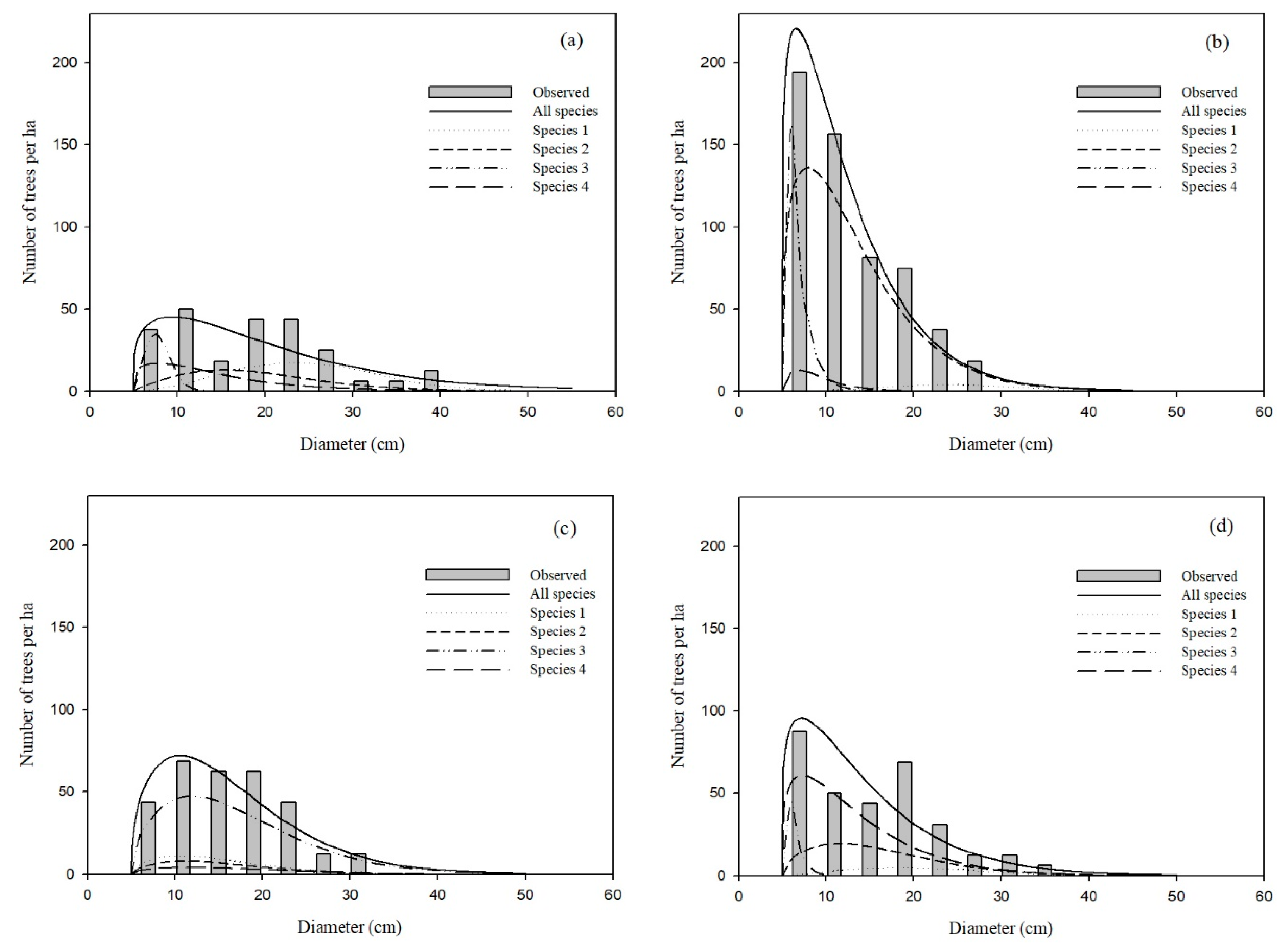
Figure 4 shows the predicted diameter distributions for each species group in four sample stands, which were dominated by species 1, 2, 3 and 4, respectively. The overall best approach, i.e., Moment Estimation using the CDFR method, was also applied at this point.

The diameter distributions of the entire stand for all four sample stands appeared to be positively skewed (Figure 4), meaning that the average age of the pine-oak mixed forests was quite young. Even though Pinus tabulaeformis (species 1) is the dominant species in Figure 4a, it also has fewer small trees than other tree species. The reason might be that Pinus tabulaeformis is a shade-intolerant species, which makes its regeneration in mixed forests relatively difficult. In contrast, small trees of Quercus aliena (species 3) frequently occur, especially in stands that are dominated by other tree species (Figure 4a,b,d). This is because Quercus aliena is shade-tolerant, and it can regenerate by both seedling and sprouting. On the other hand, Pinus armandii (species 2), which is also shade-tolerant, can only regenerate by seedling because it is a pine species, resulting in diameter distributions in between those of Pinus tabulaeformis and Quercus aliena.

Bias could be found between the predicted diameter distribution of all species and that of the summation of each species group (Figure 4). In other words, additivity was not satisfied. The average prediction error of each 4-cm diameter class using the diameter distribution model of all species were 32 trees/ha (Figure 4a), 31 trees/ha (Figure 4b), 41 trees/ha (Figure 4c) and 42 trees/ha (Figure 4d), respectively. The corresponding values by summing the diameter distribution of each species group were 25 trees/ha, 28 trees/ha, 37 trees/ha and 37 trees/ha. For the four sample stands, the prediction error was a little higher from modeling the entire stand as compared to summing distributions from individual species groups. For practical applications, Maltamo [23] suggested that diameter distribution models fitted separately for different tree species would give better predictions.

5. Conclusions

Diameter distribution models for uneven-aged pine-oak mixed forests in the Qinling Mountains of China were developed and evaluated in this study. Both Moment and Hybrid estimation approaches were used to predict the Weibull parameters. For each approach, three fitting methods (maximum likelihood estimator regression (MLER), cumulative distribution function regression (CDFR) and modified CDFR) were employed to obtain estimates for coefficients of regression equations to predict Weibull parameters. The overall results indicated that the Moment Estimation approach was better than the Hybrid approach, and that the CDFR method was superior to the MLER and modified CDFR methods. The combination of Moment Estimation and CDFR is therefore recommended for this data set.

The proposed diameter distribution models enable one to predict the diameter distribution for a given pine-oak stand in the Qinling Mountains, using limited stand information. This makes the set of models a useful tool for the inventory and management of pine-oak forests. However, different results might be obtained for other forest types. The methodology could be extended to other distributions as well.

References

- Nord-Larsen, T.; Cao, Q.V. A diameter distribution model for even-aged beech in Denmark. For. Ecol. Manag. 2006, 231, 218–225. [Google Scholar] [CrossRef]
- Diamantopoulou, M.J.; Ozcelik, R.; Crecente-Campo, F.; Eler, U. Estimation of Weibull function parameters for modelling tree diameter distribution using least squares and artificial neural networks methods. Biosyst. Eng. 2015, 133, 33–45. [Google Scholar] [CrossRef]
- De Lima, R.A.F.; Batista, J.L.F.; Prado, P.I. Modeling tree diameter distributions in natural forests: An evaluation of 10 statistical models. For. Sci. 2015, 61, 320–327. [Google Scholar] [CrossRef]
- Ozcelik, R.; Fonseca, T.J.F.; Parresol, B.R.; Eler, U. Modeling the diameter distributions of Brutian pine stands using Johnson’s S-B distribution. For. Sci. 2016, 62, 587–593. [Google Scholar]
- Meyer, H. Eine matematisch-statistiche Untersuchung über den Aufbau des Plenterwaldes. Schweiz. Z. für Forstwes. 1933, 84, 33–46, 88–103, 124–133. [Google Scholar]
- Bliss, C.I.; Reinker, K.A. A lognormal approach to diameter distributions in even-aged stands. For. Sci. 1964, 10, 350–360. [Google Scholar]
- Nelson, T.C. Diameter distribution and growth of loblolly pine. For. Sci. 1964, 10, 105–114. [Google Scholar]
- Clutter, J.L.; Bennett, F.A. Diameter distribution in old-field slash pine plantations. GA. For. Res. Counc. Rep 1965, 13, 9. [Google Scholar]
- Bailey, R.L.; Dell, T.R. Quantifying diameter distributions with the Weibull function. For. Sci. 1973, 19, 97–104. [Google Scholar]
- Tham, Å. Structure of mixed Picea abies (L.) Karst. and Betula pendula Roth. and Betula pubescens Ehrh. stands in south and middle Sweden. Scand. J. Res. 1988, 3, 355–370. [Google Scholar] [CrossRef]
- Smalley, G.W.; Bailey, R.L. Yield tables and stand structure for loblolly pine plantations in Tennessee, Alabama, and Georgia highlands. USDA For. Serv. Res. Paper SO-96 1974, 96, 81. [Google Scholar]
- Feduccia, D.P.; Dell, T.R.; Mann, W.F., Jr.; Campbell, T.E.; Polmer, B.H. Yields of Unthinned Loblolly Pine Plantations on Cutover Sites in the West. Gulf Region; Res. Pap. SO-148; US Department of Agriculture, Forest Service, Southern Forest Experiment Station: New Orleans, LA, USA, 1979; Volume 148.
- Matney, T.G.; Sullivan, A.D. Compatible stand and stock tables for thinned and unthinned loblolly pine stands. For. Sci. 1982, 28, 161–171. [Google Scholar]
- Baldwin, V.C., Jr.; Feduccia, D.P. Loblolly pine growth and yield prediction for managed West. Gulf plantations. USDA For. Serv. Res. Paper SO-236 1987, 236, 27. [Google Scholar]
- Poudel, K.P.; Cao, Q.V. Evaluation of methods to predict Weibull parameters for characterizing diameter distributions. For. Sci. 2013, 59, 243–252. [Google Scholar] [CrossRef]
- Schreuder, H.T.; Hafley, W.L.; Bennet, F.A. Yield prediction for unthinned natural slash pine stands. For. Sci. 1979, 25, 25–30. [Google Scholar]
- Brooks, J.R.; Borders, B.E.; Bailey, R.L. Predicting diameter distributions for site-prepared loblolly and slash pine plantations. South. J. Appl. 1992, 16, 130–133. [Google Scholar]
- Newton, P.F.; Lei, Y.; Zhang, S.Y. Stand-level diameter distribution yield model for black spruce plantations. For. Ecol. Manag. 2005, 209, 181–192. [Google Scholar] [CrossRef]
- Sarkkola, S.; Hökkä, H.; Laiho, R.; Päivänen, J.; Penttilä, T. Stand structural dynamics on drained peatlands dominanted by Scots pine. For. Ecol. Manag. 2005, 206, 135–152. [Google Scholar] [CrossRef]
- Jiang, L.C.; Brooks, J.R. Predicting diameter distributions for young longleaf pine plantations in southwest Georgia. South. J. Appl. For. 2009, 33, 25–28. [Google Scholar]
- Stankova, T.V.; Zlatanov, T.M. Modeling diameter distribution of Austrian black pine (Pinus nigra Arn.) plantations: A comparison of the Weibull frequency distribution function and percentile-based projection methods. Eur. J. For. Res. 2010, 129, 1169–1179. [Google Scholar] [CrossRef]
- Carretero, A.C.; Alvarez, E.T. Modelling diameter distributions of Quercus suber L. stands in “Los Alcornocales” Natural Park (Cádiz-Málaga, Spain) by using the two-parameter Weibull functions. For. Syst. 2013, 22, 15–24. [Google Scholar]
- Maltamo, M. Comparing basal area diameter distributions estimated by tree species and for the entire growing stock in a mixed stand. Silva. Fennica. 1997, 31, 53–65. [Google Scholar] [CrossRef]
- Siipilehto, J. Improving the accuracy of predicted basal-area diameter distribution in advanced stands by determining stem number. Silva. Fenn. 1999, 33, 281–301. [Google Scholar] [CrossRef]
- Chen, W.J. Tree size distribution functions of four boreal forest types for biomass mapping. For. Sci. 2004, 50, 436–449. [Google Scholar]
- Liu, F.X.; Li, F.R.; Zhang, L.J.; Jin, X.J. Modeling diameter distributions of mixed-species forest stands. Scand. J. For. Res. 2014, 29, 653–663. [Google Scholar] [CrossRef]
- Burkhart, H.E.; Tomé, M. Modeling Forest Trees and Stands; Springer Science & Business Media: Dordrecht, The Netherlands, 2012; pp. 261–272. [Google Scholar]
- Cao, Q.V. Predicting parameters of a Weibull function for modelling diameter distribution. For. Sci. 2004, 50, 682–685. [Google Scholar]
- Cao, Q.V. An integrated system for modeling tree and stand survival. Can. J. For. Res. 2017, 47, 1405–1409. [Google Scholar]
- SAS Institute, Inc. Base SAS® 9.4 Procedures Guide; SAS Institute Inc.: Cary, NC, USA, 2014. [Google Scholar]
- Anderson, T.W.; Darling, D.A. A test of goodness of fit. J. Am. Stat. Assoc. 1954, 49, 765–769. [Google Scholar] [CrossRef]
- Massey, F.J., Jr. The Kolmogorov-Smirnov test for goodness of fit. J. Am. Stat. Assoc. 1951, 46, 68–78. [Google Scholar] [CrossRef]
- Reynolds, M.R.; Burk, T.E.; Huang, W.C. Goodness-of-fit tests and model selection procedures for diameter distribution models. For. Sci. 1988, 34, 373–399. [Google Scholar]
- Weiskittel, A.R.; Hann, D.W.; Kershaw, J.A., Jr.; Vanclay, J.K. Forest Growth and Yield Modeling; John Wiley & Sons: New York, NY, USA, 2011; pp. 170–173. [Google Scholar]
- Janowiak, M.K.; Nagel, L.M.; Webster, C.R. Spatial scale and stand structure in northern hardwood forests: Implications for quantifying diameter distributions. For. Sci. 2008, 54, 497–506. [Google Scholar]
© 2019 by the authors. Licensee MDPI, Basel, Switzerland. This article is an open access article distributed under the terms and conditions of the Creative Commons Attribution (CC BY) license (http://creativecommons.org/licenses/by/4.0/).