Article

Characterizing Seedling Stands Using Leaf-Off and Leaf-On Photogrammetric Point Clouds and Hyperspectral Imagery Acquired from Unmanned Aerial Vehicle

1
Department of Forest Sciences, University of Helsinki, P. O. Box 27, 00014 Helsinki, Finland
2
Centre of Excellence in Laser Scanning Research, Finnish Geospatial Research Institute, National Land Survey, Geodeetinrinne 2, 02431 Masala, Finland
3
School of Forest Sciences, University of Eastern Finland, P. O. Box 111, 80101 Joensuu, Finland
4
Department of Remote Sensing and Photogrammetry, Finnish Geospatial Research Institute (FGI), National Land Survey of Finland (NLS), Geodeetinrinne 2, 02430 Masala, Finland
*
Author to whom correspondence should be addressed.
Forests 2019, 10(5), 415; https://doi.org/10.3390/f10050415
Submission received: 24 April 2019 / Revised: 8 May 2019 / Accepted: 8 May 2019 / Published: 13 May 2019
(This article belongs to the Special Issue Forestry Applications of Unmanned Aerial Vehicles (UAVs) 2019)

Abstract

:
Seedling stands are mainly inventoried through field measurements, which are typically laborious, expensive and time-consuming due to high tree density and small tree size. In addition, operationally used sparse density airborne laser scanning (ALS) and aerial imagery data are not sufficiently accurate for inventorying seedling stands. The use of unmanned aerial vehicles (UAVs) for forestry applications is currently in high attention and in the midst of quick development and this technology could be used to make seedling stand management more efficient. This study was designed to investigate the use of UAV-based photogrammetric point clouds and hyperspectral imagery for characterizing seedling stands in leaf-off and leaf-on conditions. The focus was in retrieving tree density and the height in young seedling stands in the southern boreal forests of Finland. After creating the canopy height model from photogrammetric point clouds using national digital terrain model based on ALS, the watershed segmentation method was applied to delineate the tree canopy boundary at individual tree level. The segments were then used to extract tree heights and spectral information. Optimal bands for calculating vegetation indices were analysed and used for species classification using the random forest method. Tree density and the mean tree height of the total and spruce trees were then estimated at the plot level. The overall tree density was underestimated by 17.5% and 20.2% in leaf-off and leaf-on conditions with the relative root mean square error (relative RMSE) of 33.5% and 26.8%, respectively. Mean tree height was underestimated by 20.8% and 7.4% (relative RMSE of 23.0% and 11.5%, and RMSE of 0.57 m and 0.29 m) in leaf-off and leaf-on conditions, respectively. The leaf-on data outperformed the leaf-off data in the estimations. The results showed that UAV imagery hold potential for reliably characterizing seedling stands and to be used to supplement or replace the laborious field inventory methods.

Graphical Abstract

1. Introduction

Sustainable forest management requires accurate and up-to-date information. The information is acquired by field measurements or remote sensing-based inventorying. The field measurements are time-consuming, expensive and laborious, in contrast to remote sensing-based inventorying techniques. Currently, unmanned aerial vehicles (UAVs, aka: drones) are in high interest for forest inventorying because of the UAVs’ capability to collect data from which suite of essential forest inventory attributes can be derived with accuracy close to field inventories [1,2,3,4,5,6,7,8]. UAVs provide an easy, inexpensive, and repeatable data collection method [9] with very high spatial resolution data that can even support the detection of small trees which has not been possible using airborne laser scanning (ALS) data [10].
In Finland, seedling stands are defined as the forest stands with mean height of < 7 m (conifer) or 9 m (deciduous) [11]. Conditions of the seedling stands can greatly predict and define the condition of future mature stands [12]. For example, Huuskonen and Hynynen [12] revealed that precommercial thinning, which was carried out when the dominate height was 3 m and the target tree density was 2000 trees per hectare (TPH), resulted in an increase of 15% in the mean diameter of the first commercial thinning. Thus, monitoring and management of the seedling stands development are required to ensure quality timber as well as the future timber supply.
ALS data, used in operational private forest inventories (61%) in Finland, is not capable to characterise seedling stands due to small tree size and high tree density. Thus, the seedling stands are inventoried by field measurements, which are the most expensive part of the total cost of the inventory. Therefore, analysing other cost-efficient means to estimate tree density, height, and species composition is required. A few studies explored the use of UAV-based photogrammetric point clouds in the seedling stands. For example, Puliti et al. [13] estimated biophysical properties of seedling stands using UAV-photogrammetric point cloud data, and compared it with ALS data. Similarly, UAV demonstrated promising results to detect coniferous seedlings in leaf-off conditions where seedlings were visually and spectrally distinctive [14]. Moreover, Goodbody et al. [15] combined UAV- and aerial-photogrammetric point clouds to assess spatial, spectral and structural details for the seedling stands. The UAV-based photogrammetric data were also utilized to investigate the feasibly and merits of UAV for evaluating regeneration performance in naturally-growing and planted conifer seedlings in different growth phases [16]; as well as assessing the effects of the European spruce bark beetle (Ips typographus L.) disturbance on natural regeneration and standing deadwood [17].
In addition to the few UAV studies, other remote sensing materials were also used for investigating the seedling stands, for example airborne imagery [18,19,20,21] and SPOT-5 satellite imagery [22]. Moreover, ALS data were applied for analysing small trees in the forest-tundra ecotone [23,24], regeneration or young forests [25,26] and predicting aboveground biomass (AGB) change in young forests [27]. Additionally, Korpela et al. [28] combined ALS and airborne imagery for characterizing seedling stand vegetation; and for detecting the requirement for tending seedling stands [29]. Also, Korhonen et al. [29] used ALS and aerial imagery to detect the tending requirement of seedling stands, by creating model function based on ALS-derived echo intensity and height percentiles together with aerial images texture. However, they appointed out that their approach could not completely replace the field visits with regards to the need for tending seedling stands.
The use of hyperspectral data and comparing data from leaf-off and leaf-on conditions remained unexplored in the previous seedling-focused studies. Thus, this study was designed to extend current knowledge of using UAV-red, green, blue (RGB)-imagery, UAV-hyperspectral data as well as analysing the performance of leaf-off and leaf-on data with predefined plot-level tree densities (TPH). This research concentrates on retrieving the total and spruce-specific tree density and height in seedling stands in the southern boreal forests of Finland. We focused on the spruces because it is the species of interest to be grown and spruce seedling stands commonly require more care (e.g., tending and removal of naturally regenerated broadleaf trees) compared to seedling stands of Scots pine. In Finland, seedling stands are divided into young (height ≤  1.3 m, YoS) and advanced seedling stands (height  >  1.3 m, AdS). Therefore, this study also aims to assess the differences between predictions for YoS and AdS.

2. Materials and Methods

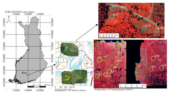
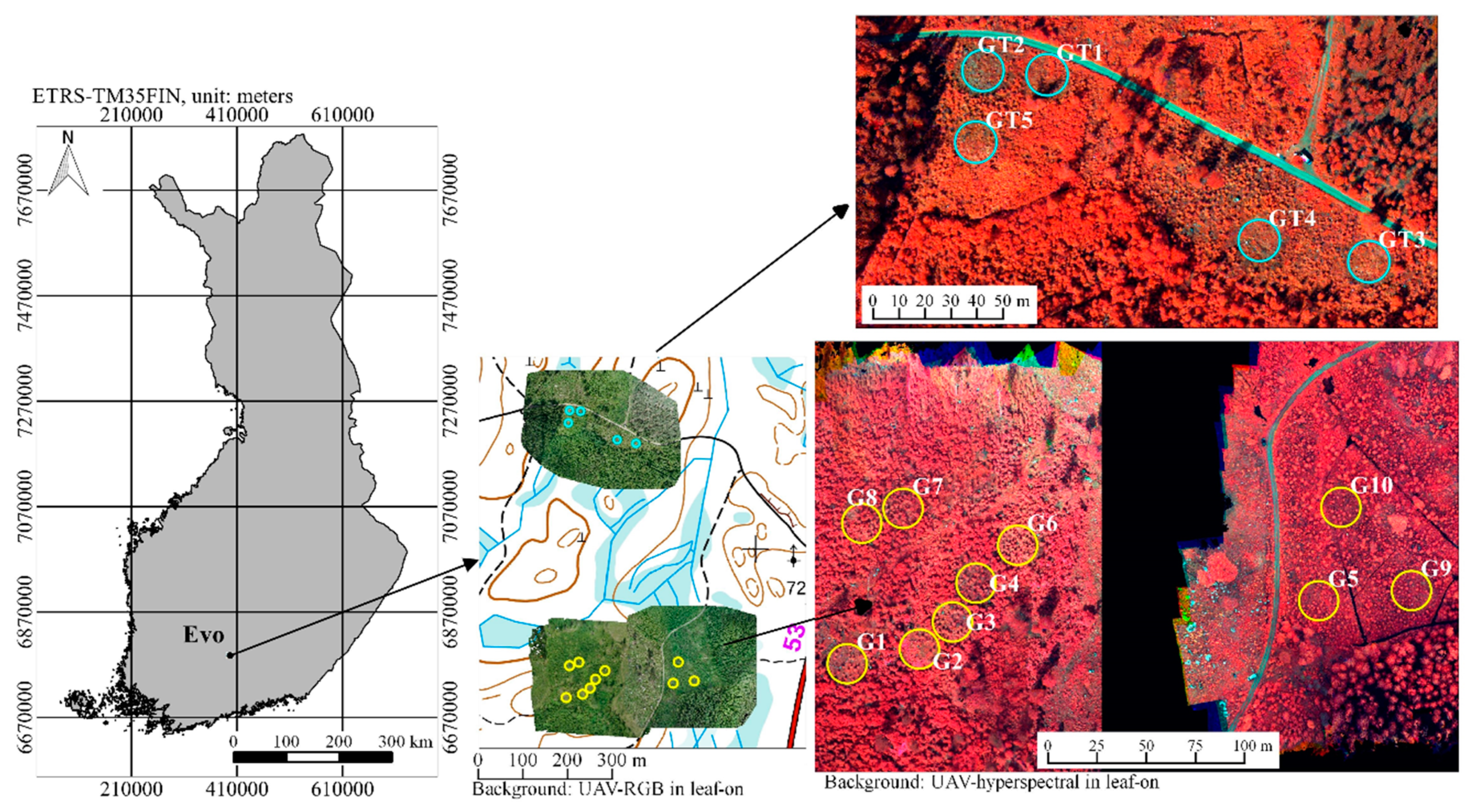
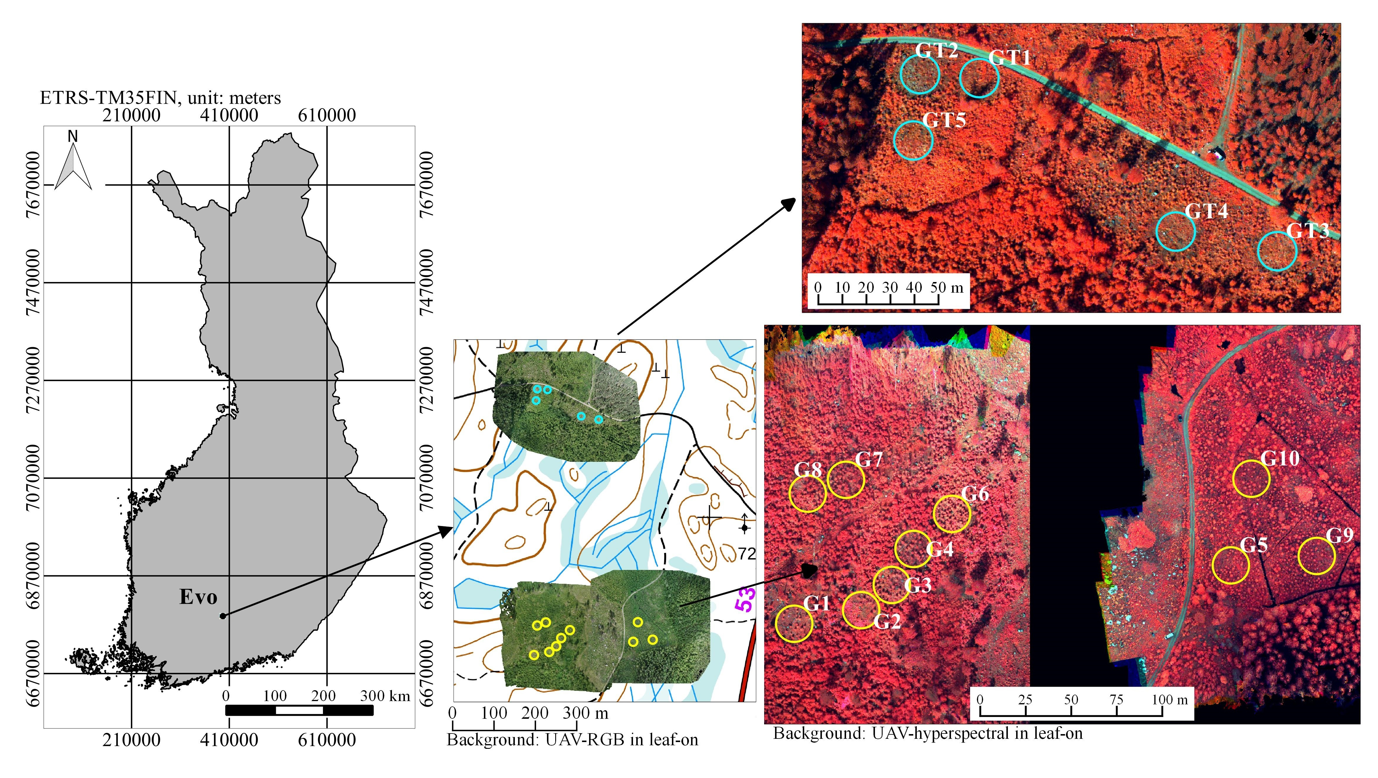
2.1. Study Area and Establishment of the Sample Plots

This study was carried out in a southern boreal forest zone in Evo, Finland (61.20° N, 25.08° E, 133–150 m above sea level) (Figure 1). There are mostly managed forests where Scots pine and Norway spruce are the dominant tree species.
In our study, we selected one YoS and one AdS stand from the study area based on the existing forest resource information. A prerequisite for both seedling stands was the number of TPH, which had to be more than 2400. Such a density was required to establish sample plots and thin them to varying densities. We established five sample plots with an 8-m radius to YoS and 10 sample plots with a 10-m radius to AdS. The sample plots in YoS were thinned approximately to the following target tree densities: 1200, 1400, 1600, 1800, and 2000 TPH. Respectively, the sample plots in AdS were thinned to the following densities: 600, 800, 1000, 1200, 1400, 1600, 1800, 2000, 2200, and 2400 TPH.
The sample plots were established in April through May 2016. Sample plot locations were recorded using the Trimble GeoXT Global Navigation Satellite System (GNSS) device. The GNSS positions were differentially corrected using the data from the local reference station. The expected accuracy in an open area is below 1 meter. After the thinning treatments, tree attributes were measured during June (Table 1), and the sample plot-level forest inventory attributes were compiled. In YoS all remaining trees were spruce, but AdS sample plots had an admixture of birch that varied from 0% to 51%. The site type of our sample plots is the mesic heath forest.
During the field data collection in June, many fern and grasses had emerged. In AdS, the tree species was determined, and the diameter at breast height (DBH) was measured with steel callipers from every tree with a height of ≥ 1.3 m. The tree height was measured using an electronic hypsometer (Vertex IV, Haglöf, Långsele, Sweden) from every third tree for each tree species. In addition, the height of the tallest tree was measured from every sample plot. YoS was measured similarly, but instead of DBH, the diameter at ground height was measured because the mean height of the YoS sample plots was less than 1.3 m (Table 1). The height for all of the trees within each sample plot was predicted using the sample tree height measurements and by fitting the Näslund’s height curve [30] to the measured data. The relative RMSE of the tree height prediction was 12.8% (relative Bias: −0.13%) and 11.8% (relative Bias: 0.60%) for YoS and AdS, respectively. In the sample plots with mixed species classes, mean tree height of all trees was calculated with a weighted average of the number of each tree species and their mean height. Plot-level TPH was calculated by dividing the number of field-observed trees in each plot with its area (radius of 8 and 10 m in YoS and AdS, respectively) and converting the area to hectare. Species-specific tree height and TPH statistics are presented in Table 1.

2.2. Remote Sensing Data

Remote sensing data acquisition were carried out using a hexacopter drone of the Finnish Geospatial Research Institute (FGI). A hyperspectral camera based on Fabry–Pérot interferometer (FPI) [31] and a Samsung NX300 RGB camera were used to collect remote sensing imagery. The FPI technology provides spectral data cubes with a rectangular image format, but each band in the data cube has a slightly different position and orientation. The sensor provides images with dimension of 1024 in 648 pixels where every pixel is 11 μm × 11 μm. In this study, a filter with a wavelength range of 500–900 nm and settings with 36 separate bands was used; the spectral resolution range was 10–40 nm at the full width at half maximum (FWHM) (Table 2). A Samsung RGB camera had a 16-mm fixed lens and an image size of 5472 × 3648 pixels. The drone was equipped with a NV08C-CSM-GNSS receiver that was used to calculate the flight trajectory. The Raspberry Pi2 on-board computer was used for collecting timing data for all devices and for logging the GNSS receiver. More details of the imaging sensor and UAV system are provided in [32,33].
The UAV imagery was acquired during leaf-off (9 and 11 May) and leaf-on (29 June) 2016 in three separate flights in both seasons. The weather conditions were bright and cloudless during leaf-off campaigns and varied from sunny to cloudy during leaf-on campaigns (Table 3). The flight height was 100 m from the ground level, which provided a ground sampling distance (GSD) of 10 cm for the FPI and 2.5 cm for the RGB images. The flight speed was 3 m/s. The forward and side overlaps were 83% and 80%, respectively, for the FPI camera blocks and 96% and 85%, respectively, for the RGB camera blocks. Altogether, 20 ground control points (GCPs) were installed in the areas for georeferencing purposes (6 GCPs in YoS and 7 GCPs in both AdS east and west). They were targeted with circular targets with a 30-cm diameter, and their coordinates were measured using a Trimble R10 (L1 + L2) RTK-GPS receiver with accuracies of 2 cm in horizontal coordinates and 3 cm in height. For the reflectance transformation purposes, reflectance panels with a size of 1 m × 1 m and nominal reflectance of 0.03, 0.10, and 0.50 [34] were positioned near the UAV take-off place. An ASD Field Spec Pro (Analytical Spectral Devices, Malvern Panalytical Ltd., Malvern, United Kingdom) with cosine collector optics was installed near the take-off place to make irradiance measurements during the flights.

2.3. Creating Dense Point Clouds and Image Mosaics

Georeferencing of the RGB images was carried out using the Pix4D MapperPro (Pix4D S.A., Prilly, Switzerland) version 2.2.25 software and supported by GCP and GNSS trajectory data collected on-board the UAV. After orientation processing, dense three-dimensional (3D) point clouds were created by automatic image matching using average point densities of 1600 points/m2. Orientations of the FPI images were determined in a separate process. First, the orientations of three reference bands (band 3: L0 = 513.5 nm; band 11: L0 = 591.9; band 14: L0 = 616.2 nm) were calculated using the Pix4D software, as was the case with the RGB images. The rest of the bands were co-registered to the reference bands using a rigorous 3D approach [35]. The process provided the band registration with a better than 1-pixel accuracy over the area.
The objective of the radiometric processing of the FPI imagery was to provide high-quality reflectance mosaics including the 36 spectral bands. The radiometric modelling approach developed at the FGI and implemented in the FGI’s radBA software (version 2016-08-20, Masala, Finland), an in-house toolbox for radiometric block adjustment [32,36], included sensor correction, atmospheric correction, correction for the illumination changes and other non-uniformities, and normalisation of the anisotropy effects due to the varying illumination and viewing directions [32]. The empirical line method [37] was used to calculate the transformation from digital numbers to reflectance factors with the aid of the reflectance reference panels. A radiometric block-adjustment method was used to determine the model-based radiometric correction to compensate for the radiometric disturbances. In this investigation, the relative image-wise correction parameters were calculated for all six datasets. Furthermore, disturbances caused by the object-reflectance anisotropy (i.e., bidirectional reflectance distribution function (BRDF)) were determined for the datasets that were collected during sunny weather (Table 3). Markelin et al. [38] previously evaluated different options of the radiometric processing.
The RGB image orthomosaics were calculated with a GSD of 2.5 cm using the Pix4D software. The hyperspectral orthomosaics were created using the FGI’s radBA software ([32,36] with a GSD of 10 cm).

2.4. Delineation of Tree Crowns and Extracting 3D Metrics

The height of the photogrammetric point clouds was normalised to the height above-ground level using the national digital terrain model (DTM) with the resolution of 2 m. The DTM was created by the National Land Survey of Finland using ALS data. The expected elevation accuracy of the DTM varies from 10 to 30 cm in boreal forest conditions [39]. The DTM has been updated in August 2015.
For detecting tree crowns, leaf-off and leaf-on canopy height models (CHMs) were created from the normalised point clouds, by assigning the height value of the highest point to pixels of the CHMs. The resolution of 10 cm was selected for the CHMs to also match with the resolution of the FPI hyperspectral images. To avoid any empty pixels (gaps) in the CHMs, values for the null pixels were interpolated using the K-nearest neighbour inverse distance weighting (KNNidw) with the three nearest neighbours in the lidR package [40] in R 3.3.3 [41]. To delineate tree crowns from the CHMs of each plot, we applied watershed segmentation in SAGA GIS version 2.3.2 [42].
The maximum and mean height (Hmax, Hmean) of segments were extracted from CHMs. Then, segments with Hmax below a height threshold (0.5 m and 1.0 m for YoS and AdS, respectively) were excluded as ground vegetation or understory. Næsset and Bjerknes [26], and Økseter et al. [27], excluded ALS points below the 0.5-m threshold, assuming them to be laser returns from the ground vegetation. Therefore, we selected the threshold 0.5 for YoS and 1m AdS. Moreover, according to field data (Table 1), the smallest tree had Hmin of 0.73 m in YoS and 1.57 m in AdS. Therefore, the selected thresholds were lower to include all tree segments. Within segments, we kept cells with height of ≥ 50% of segments Hmax to minimise the possible effect of understory. The 50% was selected by expert knowledge and visual inspection, although we admit that there might be other approaches.

2.5. Selection of Training Segments

The exclusion of segments with Hmax below height thresholds was also applied for segments located outside sample plots boundary. Then, training segments were selected by visual interpretation of the well-distinguishable and typical leaf-off and leaf-on segments, located within a 2 m buffer around the sample plots boundary. The visual interpretation was carried out using leaf-off and leaf-on RGB orthomosaics to detect tree classes (spruce and birch) and non-tree classes (stumps/deadwood, bush/grass and rock). The number of training segments were 144 in leaf-off and 279 in leaf-on (Table 4). The non-tree classes were merged for the classification step.
The number of training data is higher in leaf-on (Table 4) because grass, bushes, and ferns (which are in the non-tree class) had more segments in leaf-on data. They emerge in summer, grow fast, and reach the height thresholds.

2.6. Vegetation Indices and Finding Optimal Bands

We calculated the arithmetic mean of spectral values for each band from the hyperspectral data for each segment in the leaf-off and leaf-on data separately. These were then used to calculate three vegetation indices (VIs) (Equation (1)) using a combination of near-infra red (NIR) together with green (i), red (ii), and red-edge bands (iii). As there were several bands within these ranges of spectrum in our hyperspectral data (Table 5), we calculated all possible combinations of the three VIs using Equation (1).
Index = ( R λ 1 R λ 2 ) ( R λ 1 + R λ 2 ) ,
where R is the reflectance value and λ1 and λ2 are the wavelengths of the two bands employed in the index.
To select the optimal and most important bands for the VIs in identifying trees from non-trees as well as spruce from birch, we ran the random forest method (implemented from yaImpute package [43] in R 3.3.3) 100 times for both leaf-off and leaf-on data. The final selection for the VIs was done based on the scaled importance; in other words, the VIs that were considered the most important variable at least 20 times of the 100 random forest runs were selected for the final modelling.

2.7. Segments Classification

In addition to the optimal VIs, Hmax and Hmean were also used as predictors in training and prediction phases of the random forest classification method [44] to predict the species class of segments. The random forest classification method was applied to find the nearest neighbours (i.e., crown segments) in a feature space using the predictors selected (i.e., VIs, Hmax, and Hmean).
We used the random forest method from the yaImpute R package with the buildClasses mode with 500 trees, k = 1, and we set the classification classes (birch, spruce, non-tree classes) as the y variable.
After classifying the segments, we discarded non-tree classes and proceeded to extract the plot-level total and spruce-specific TPH, as well as the mean height of all trees and of spruce trees’ mean height. Note that tree heights were derived from CHMs and not predicted with the random forest method.

2.8. Accuracy Evaluation for Tree Density and Height

We compared plot-level spruce-specific TPH and the total TPH attributes with field-measured reference. To evaluate the reliability of remotely sensed tree height, we compared our estimation of the plot-level mean tree height with its corresponding field data, either spruce-specific tree heights or total tree heights, using the equations. Absolute and relative bias (BIAS) and RMSE were calculated for each attribute (Equations (2)–(5)).
BIAS = i = 1 n ( y i y ^ i ) n ,
BIAS % = 100 × BIAS y ¯ ,
RMSE = i = 1 n ( y i y ^ i ) n ,
RMSE % = 100 × RMSE y ¯ ,
where n is the number of plots, yi the value from the field data for plot i, y ^ i the remotely sensed (predicted) value for plot i, and y ¯ is the mean of the variable in the field data.
In addition, we also used Pearson correlation coefficient (r). The output value can be interpreted as the proportion of the variance in an attribute (remotely-sensed data) to the variance in another (field data) as x and y, respectively. The formula is the following:
r = i = 1 n ( x i x ¯ ) . ( y i y ¯ ) i = 1 n ( x i x ¯ ) 2 . i = 1 n ( y i y ¯ ) 2 ,
The accuracy evaluation for TPH and tree height was analysed and reported for all sample plots (n = 15) for both leaf-off and leaf-on conditions. Additionally, the accuracy was assessed among YoS (n = 5) and AdS (n = 10) separately.

3. Results

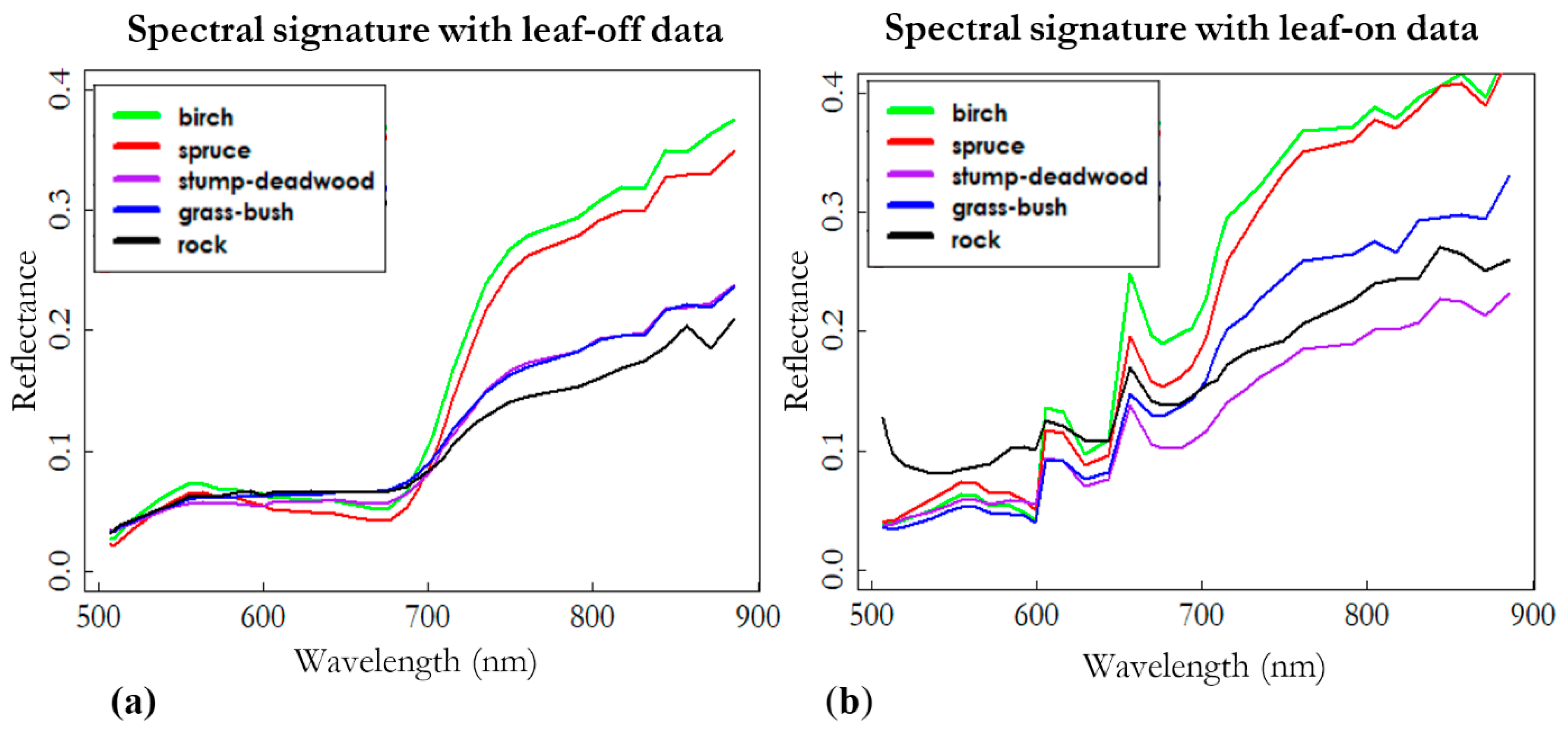
3.1. Analysing Spectral Features and Optimal Bands for Vegetation Indices

The spectral reflectance of training data using leaf-off and leaf-on hyperspectral data (Figure 2) showed that the tree classes are distinguishable from the non-tree class, especially in the red-edge and NIR spectrum in both epochs. The reflectance spectra from AdS leaf-on datasets had some anomalies (Figure 2b). The datasets were captured under cloudy or partially cloudy conditions using a short exposure time of 10 ms, which resulted in poor image quality, especially in the red spectral range (600–670 nm). This was not considered a critical problem in the analysis because only one of the indices was in this range, and our selection procedure did not select the lowest quality bands for the indices.
The optimal bands found and used for creating VIs are given in Table 6 for each epoch.

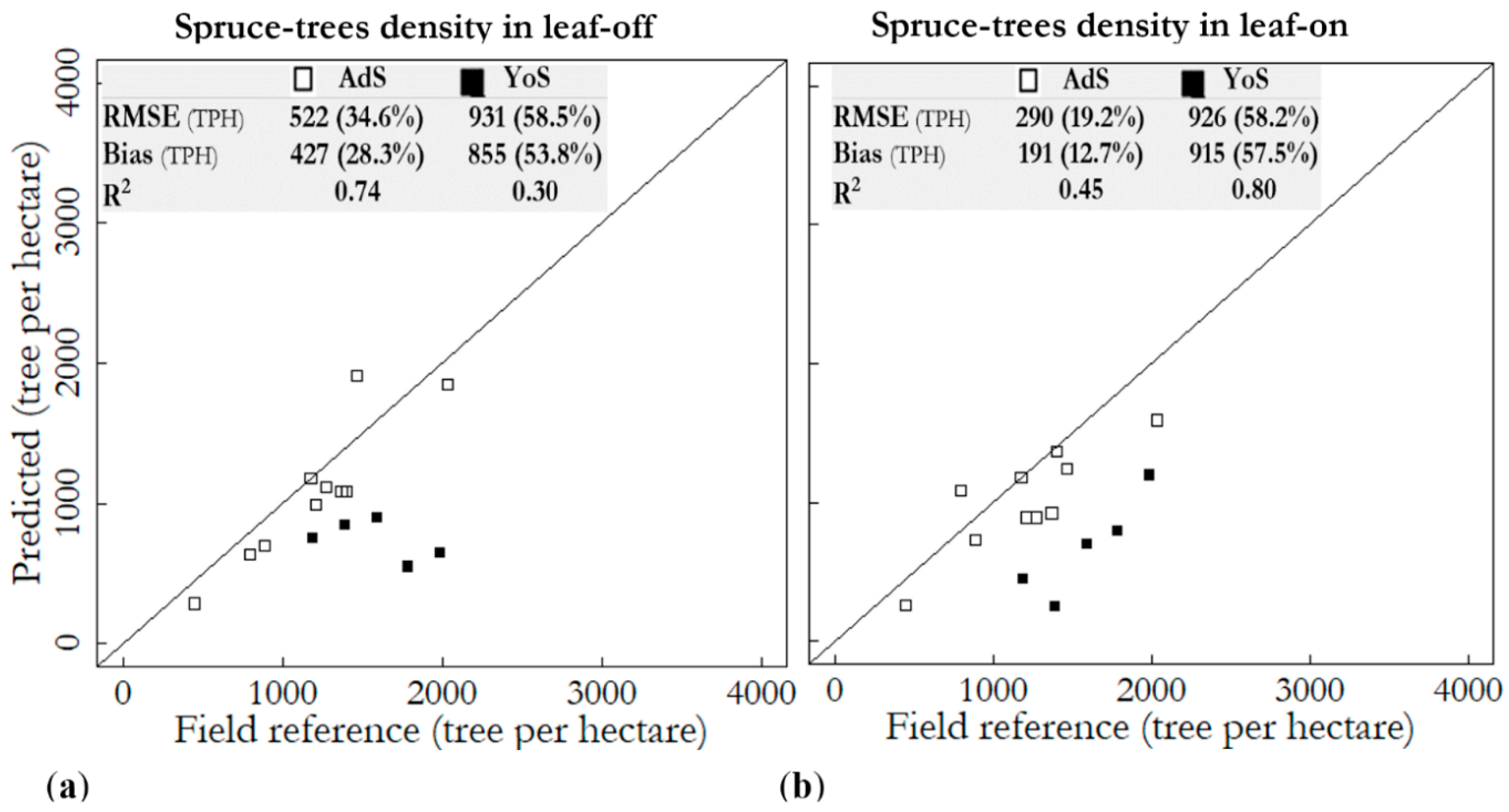
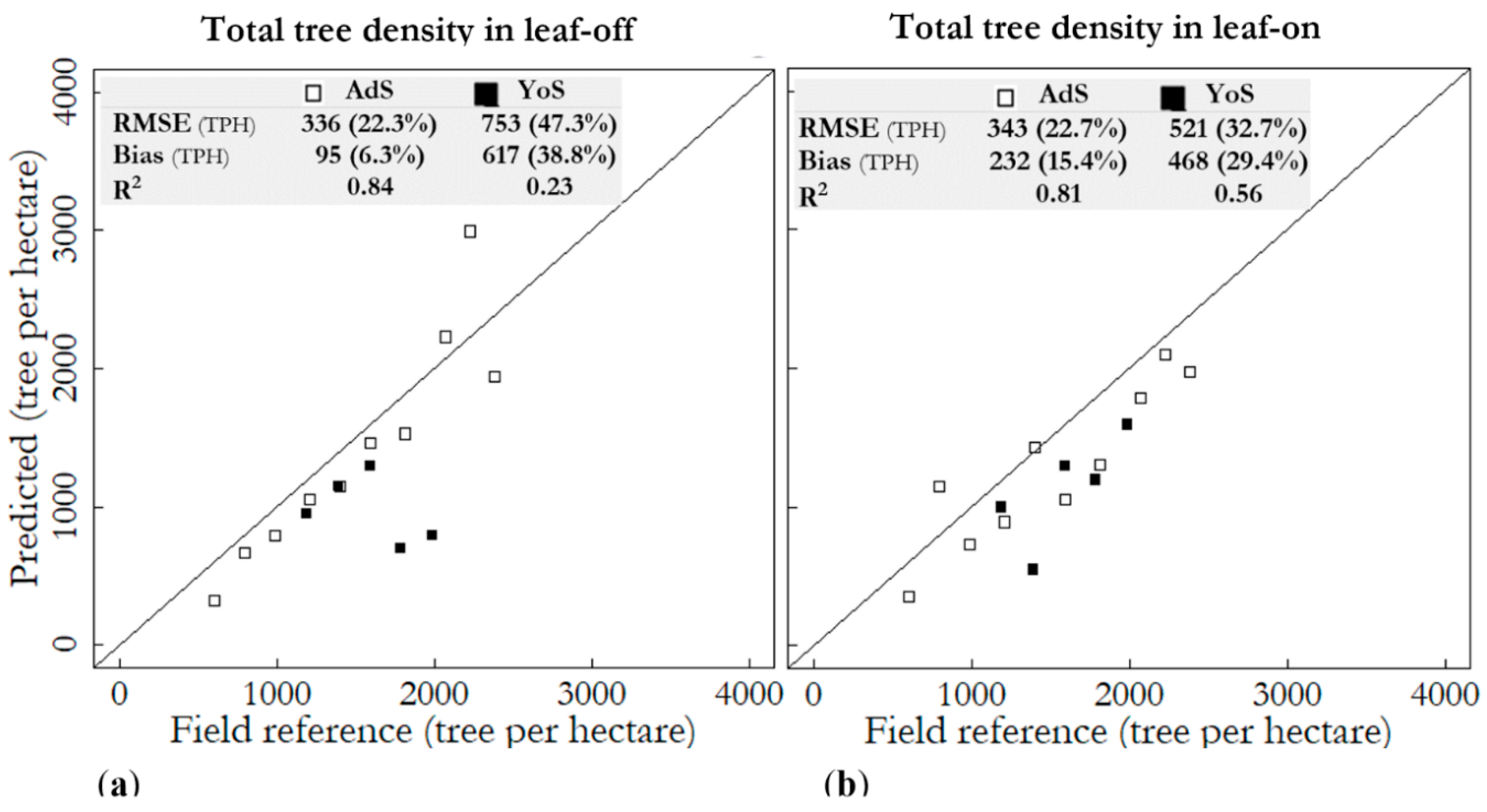
3.2. Tree Density Estimation

Both total tree density and spruce tree density were more accurately predicted with leaf-on data (Table 7). The total tree density was estimated approximately 10%-points more accurately (relative RMSE of 33.5% and 26.8% in leaf-off and leaf-on) than spruce tree density (44.6% and 38.1%) in both epochs.
The estimation of the total TPH was also compared among YoS and AdS separately (Figure 3). Total tree density of YoS were estimated more accurately with leaf-on data (relative RMSE of 32.7%) than with leaf-off data (relative RMSE of 47.3%). The total TPH was underestimated by 15.4% in leaf-on conditions whereas the underestimate for leaf-off conditions was 6.3%; although there was no substantial difference in relative and absolute RMSE between the epochs (Figure 3).
Moreover, spruce tree density among YoS (n = 5) and AdS (n = 10) was also calculated for both epochs (Figure 4). The relative RMSE of spruce tree density in AdS was 19.2% in leaf-on data whereas it was 58.5% and 58.2% in YoS for both epochs. Spruce tree density was less underestimated in AdS in leaf-on (28.3% and 12.7% in leaf-off and leaf-on); nevertheless, it was approximately 4%-points more accurate in leaf-off in YoS (53.8% and 57.5% in leaf-off and leaf-on conditions).

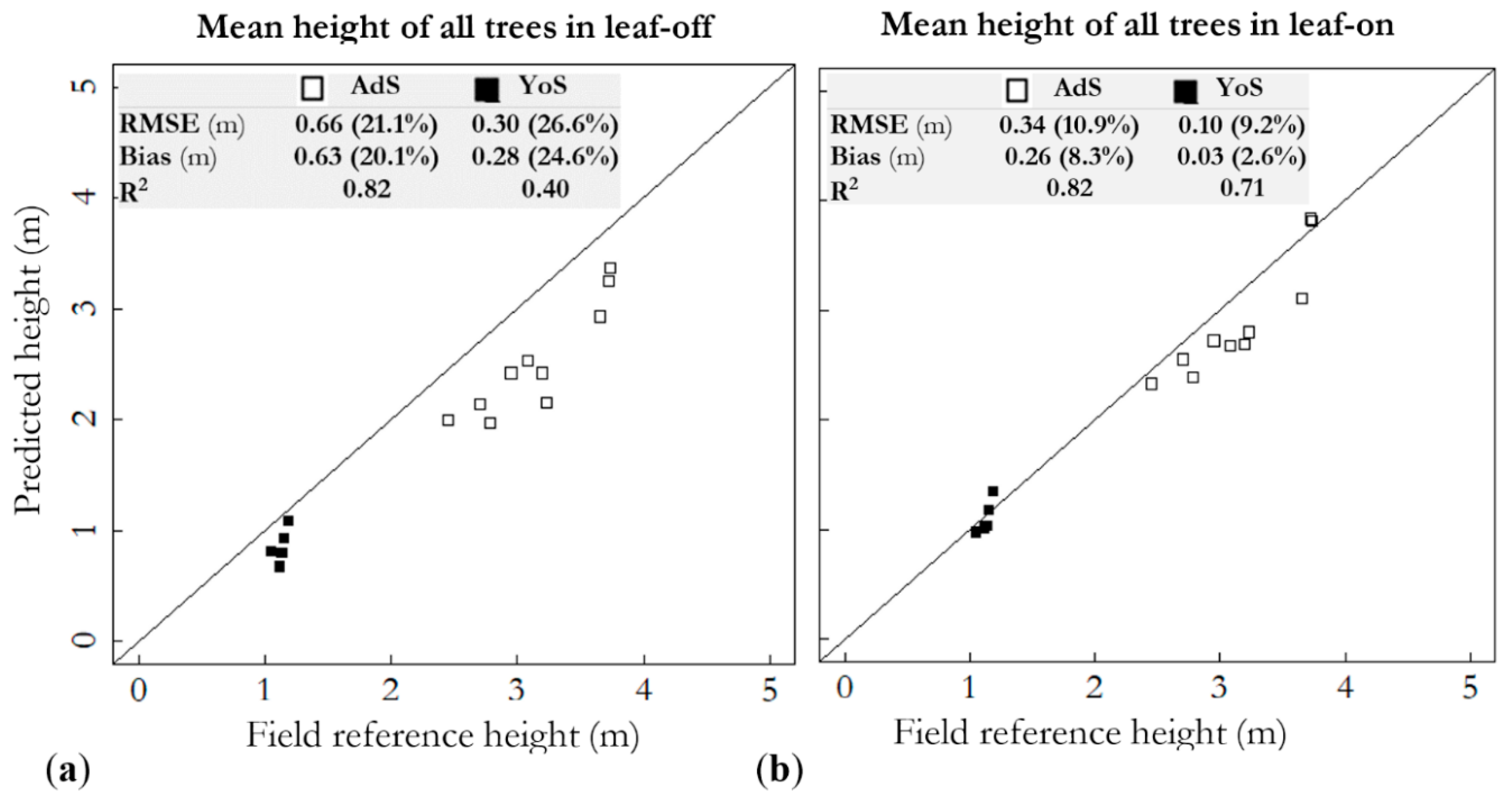
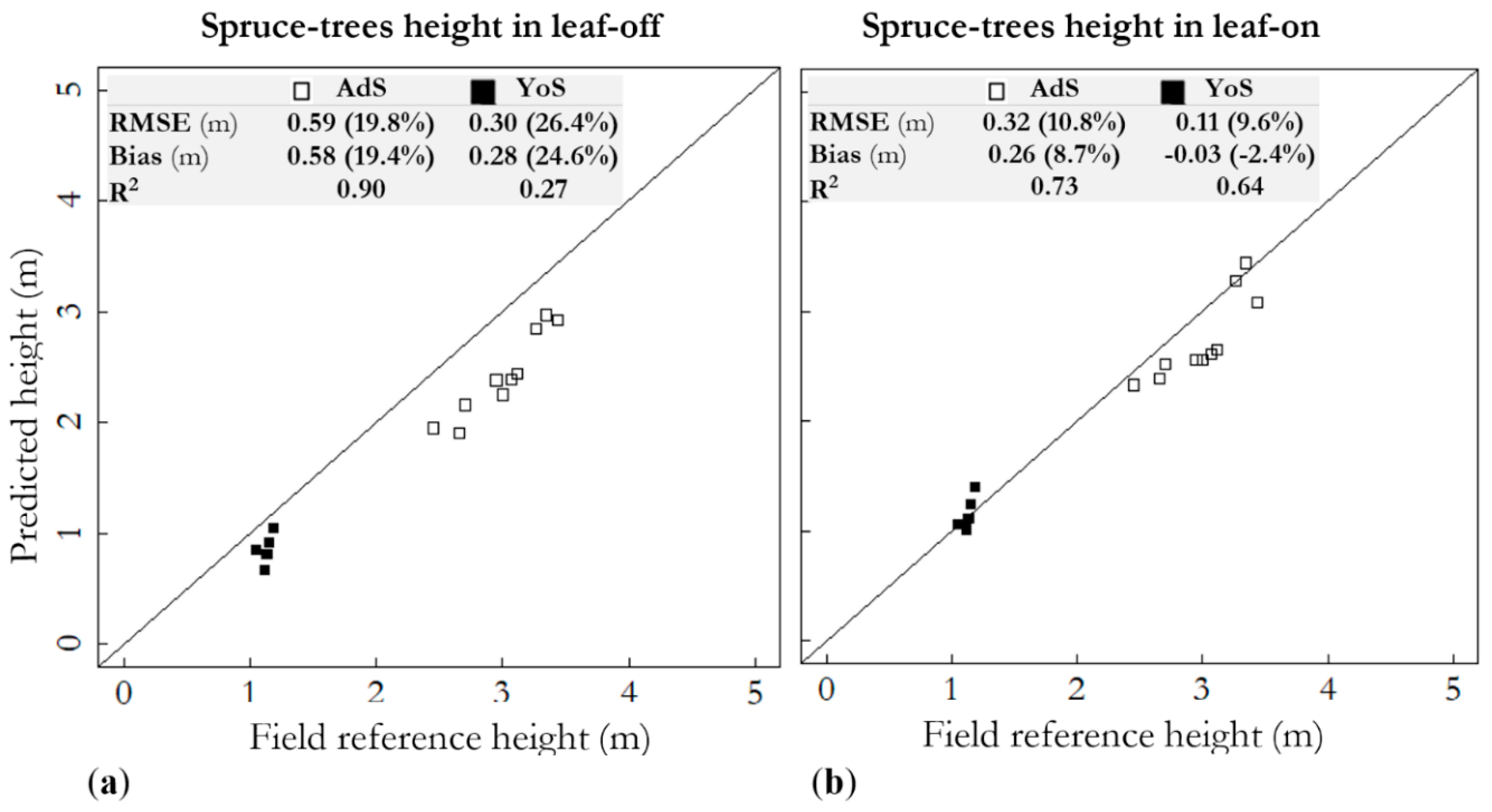
3.3. Height Attribute Extraction

Among all sample plots, the mean height of all trees was underestimated by 20.8% and 7.4% (relative RMSE of 23.0% and 11.5%) in leaf-off and leaf-on conditions, respectively (Table 8). The mean height of spruces was underestimated by 20.2% and 6.9% (relative RMSE of 21.7% and 11.4%) with leaf-off and leaf-on data, respectively. As the results show, leaf-on data were more favourable for both all trees and the spruce mean height estimation. The absolute RMSEs and biases were 0.29 m and 0.18 m, respectively, for the leaf-on data, and 0.57 m and 0.52 m, respectively, for the leaf-off dataset.
Figure 5 shows the estimation of the total tree height among YoS and AdS separately in both epochs. Leaf-on data resulted in more accurate estimations in both YoS and AdS. The mean height of all trees in AdS was underestimated by 20.1% in leaf-off, whereas it was improved to 8.3% in the leaf-on data. The underestimation in YoS was improved from 24.6% in leaf-off conditions to 2.6% in leaf-on conditions.
The mean height of spruces was underestimated by 19.4% and 8.7% (relative RMSE of 19.8% and 10.8%) in the AdS in leaf-off and leaf-on conditions, respectively (Figure 6). Although it was underestimated by 24.6% (relative RMSE of 26.4%) for the YoS in leaf-off conditions; it was overestimated by 2.4% in leaf-on conditions (relative RMSE of 9.6%). The overestimation (Figure 6b) could be due to higher underestimation of spruce tree density in leaf-on (Figure 4b), which could show the omission of small spruce trees and result in the 2.4% overestimation. Relative RMSE for AdS (10.8%) was larger than YoS (9.6%) in leaf-on, in contrast to leaf-off conditions.

4. Discussion

4.1. Tree Density Estimation

Our findings for total trees density in leaf-on (relative RMSE: 26.8%) was an improvement to [13] that achieved plot-level relative RMSE of 36.3%, that used area-based approach to fit random forest models with plot data and UAV for estimating forest attributes. We shall note that Puliti et al. [13] presented RMSE of different tree densities ranging between 1 to >10,000 at every 1000 intervals. Comparing the range of our field tree density (600–2400 TPH) with the corresponding reported interval in their results, our total tree leaf-on RMSE was more accurate (411 TPH) than their achievement (~1900 TPH). Our underestimation of tree density (leaf-off 17.5% and 20.2% leaf-on) was greater than [14] (13.6%). The greater underestimation can be because of different tree detection method they used three-step object-based methods, unlike our watershed-segmentation.
Comparing our findings with seedling-focused ALS studies, our relative RMSE was more accurate (26.8%) than [13] (53.4%). They used ALS data with point density of 5 points m−2 with the same methodology that they used for UAV data, area-based approach and random forest model fitting. Our higher point density and the different used method could consequence the outperformance. Earlier, Ørka et al. [25] applied ALS for predicting the attributes of 19 regeneration stands achieved a relative RMSE of 47% for predicting the total TPH at the stand level. Comparing our plot-level results with that of the stand level predictions in [25], our findings are more accurate because a decrease in the RMSE values was observed when scaling the plot-level estimation to stand level [13]. Moreover, an earlier study [26] utilised small-footprint ALS to estimate the tree height and the TPH in young forest stands (tree heights < 6 m). They resulted in a relative RMSE of 42% for predicting the stem number using a regression model, created with a combination of field reference data. Our tree density results (relative RMSE: 26.8%) were more reliable than above-mentioned studies in the seedling stands. However, we admit that every study can have various parameters that affect the results, such as sample size, tree species, density and height conditions, different resolution and quality of remote sensing imagery. The most comparable studies are [13,14], because the other above-mentioned literature used models to predict TPH, instead of direct detection of the trees from the remote sensing data.

4.2. Tree Height Estimation

Our findings for total trees leaf-on height (relative RMSE: 26.8% TPH) was in line with [13], achieved plot-level relative RMSE of 30.9 % using area-based approach and fitting random forest models with plot data and UAV to predict forest attributes. Our tree height estimation was more accurate than [17] that used UAV-based photogrammetric point clouds to assess the effects of the European spruce bark beetle (Ips typographus L.) disturbance on natural regeneration and standing deadwood. They reached a mean RMSE of 1.31 m (59%) and 1.57 m (64%) for manually and automatically delineated regeneration trees, respectively. They reported more accurate tree height estimation with point clouds from UAV than from aerial photography (mean relative RMSE of 115% and 59%, respectively), when manually delineating trees in both data. Moreover, Vepakomma et al. [16] resulted in an underestimation of 0.39 m in seedling tree height retrieval using UAV-based photogrammetric point clouds. Furthermore, Goodbody et al. [15] assessed the conditions of regeneration stands using digital aerial photography and UAVs, and underestimated tree height by 0.55 m (RMSE = 0.92 m) using UAV-based photogrammetric point clouds. They claimed that their result had the potential to be used in silvicultural prescriptions and growth projection models.
ALS has been another important data source for estimating tree height. Puliti et al. [13] achieved 32.0% of relative RMSE when assessing seedling tree height using 5 points m−2 density ALS data. Also, Ørka et al. [25] utilised ALS data in 19 regenerations stands in Norway for predicting tree attributes. They revealed relative RMSE of 28% for predicting the mean tree height at the stand level. Næsset and Bjerknes [26] predicted the plot-level height with 0.23 m (3.5%) of bias using a two-stage procedure. Note that only 29 sample plots (of the total 174 sample plots of their whole study area) were young stands (heights < 11.5m). Also, the tree height in the study [26] was higher than this study, although their tree density was higher (mean density 4197 TPH). Their smaller bias could be due to the two-stage procedure or because they had a mixture of mature stands in their study.
In our evaluations, the absolute RMSE and bias for mean tree height of all trees were 0.29 m and 0.18 m, respectively, for the leaf-on data, and 0.57 m and 0.52 m, respectively, for the leaf-off dataset. The values of the leaf-on data were close to the limits of the methods when considering the georeferencing accuracy of approximately 0.05 m, reconstruction accuracy of the tree surfaces of decimetres, and the uncertainty of the ALS based DTM, of approximately 0.10–0.30 m. The poorer accuracy of the leaf-off data is likely to be due to the challenges of 3D object reconstruction of leafless branches with of data set with a GSD of 2.5 cm using image matching; furthermore, the overall accuracy of the photogrammetric processing could be poorer with the more challenging leaf-off dataset. These results were better than in earlier studies for seedling stands although the earlier studies can have different parameters that can influence on the result such as sample size, tree species, density and height conditions, in addition to the quality of remotely-sensed data. The mean tree height in [17] varied between 1.19 and 4.10 m within eight sample plots, scanned by UAV at 40-m flying altitude. The GSD after optimisation process in the study had yielded average residuals < 10 cm in all plots (they used only RGB, not hyperspectral). Yet the flight height in this study was 100 m, which resulted in a GSD of hyperspectral data up to 10 cm and RGB-orthomosaics of 2.5 cm. The regeneration density in the study [17] varied more (approximately 300–8000 TPH) than in this study (approximately 1200–2000 TPH in YoS and 600–2400 TPH in AdS). Yet in this study, the deviation of plot-level tree height was higher (0.77–4.54 m) than in [17] that varied between 1.19–4.10 m.
In this study, the tree height could be even more accurately estimated if our field reference data were measured at the individual tree level or if at least the training data had tree-wise field-measured height. It is common that the tree height is also predicted at the same time as species classification carries out using the random forest method because it can handle predicting several attributes. This could improve the height estimation further and correct the small overestimation of tree height in YoS in the leaf-on data. Additionally, underestimation in tree density can cause overestimation in height retrieval, especially the omission of smaller trees. It was perhaps why the underestimation of spruce density in leaf-on caused a minor height overestimation (2.4%).

4.3. Comparing Leaf-Off and Leaf-On Data

This research was specifically designed to evaluate the performance of data collected in leaf-off and leaf-on conditions for seedling stands. It was observed that inventorying in leaf-on conditions is more favourable for both tree density and mean tree height overall, and we recommend the use of leaf-on data when object reconstruction is based on photogrammetry. Mean tree height was predicted more reliably (relative RMSE: 11.5%) than tree density (relative RMSE: 26.8%) among all sample plots with leaf-on data.
To the best of our knowledge, there were no prior literature to compare leaf-off and leaf-on data for characterizing seedling stands (using any type of remote sensing data, either from UAV, aerial imagery, active sensing or spaceborne). Therefore, we should compare our findings with studies that focused on non-seedling stands. In mature forests, leaf-off and leaf-on aerial images had been used to assess mapping of forest attributes [45]. They recommended against of using leaf-off aerial images, where coniferous trees (pine and spruce) were major species with birch trees as minor tree, because they observed poor accuracy and underestimation of height distribution using leaf-off data in deciduous forest. The lower height value estimation in leaf-off data was also reported by [46], that used leaf-off and leaf-on aerial images to estimate the proportion of deciduous stem volume in mixed coniferous-deciduous forest using area-based approach. Our findings are in parallel with their results. It is worth noting that further advantage of the leaf-on data includes the prospects of utilizing the spectral information in characterizing the vegetation.
In terms of ALS data for mature forests, small difference (relative RMSE and bias < 2%) was reported for estimating all forest attributes except volume (< 7%) between leaf-off and leaf-on data, affirming that leaf-off ALS data could be used for area-based methods [47]. Similarly, Lorey’s mean height were estimated more accurately in leaf-off (RMSE: 0.07 m), than leaf-on (RMSE: 0.09 m) using area-based approach with ALS in a mixed managed boreal forest [48]. Also, other ALS studies recommended the use of leaf-off [49,50]. The reported slight advantage of leaf-off data in the ALS studies could be due to the used single-spectral ALS sensor that can be insufficient for discriminating different species in leaf-on conditions; in contrast to multi- and hyper-spectral data that outperformed in leaf-on in our research as well as other studies [45,46]. We note that further studies are required to examine this with more sample plots.
Our study showed that UAV imagery can be reliable used for characterizing seedling stands and may be a supplement or replacement for inventorying seedling stands in the future. Admittedly, further studies with more sample plots containing more deviation in tree height and density are required.

5. Conclusions

We used UAV-based photogrammetric point clouds and hyperspectral data to characterize tree attributes in seedling stands with our predesigned tree density and the species proportions of each field plot. Our data were acquired with leaf-on and leaf-off conditions.
Tree density feature in AdS were more accurately predicted compared to YoS, although tree density was higher in AdS. Thus, it can be concluded that the YoS (average height of less than 1.3 m) remained challenging to UAV-based photogrammetric point clouds and hyperspectral data and required further studies with more sample plots.
Overall, mean tree height of all and spruce trees were estimated more accurately in leaf-on conditions for both YoS and AdS. Comparing both height estimations between YoS and AdS in leaf-on conditions, the heights were estimated more accurately for YoS than AdS.
Comparing epochs, it can be concluded that collecting remotely sensed data in leaf-on conditions could be more favorable because our findings showed lower absolute and relative RMSE with leaf-on data for both the total and spruce tree density. The superiority of the leaf-on condition, considering absolute and relative RMSE, was the same for mean tree height of all and spruces trees, for both YoS and AdS, although some absolute and relative bias were different. Generally, leaf-on data is recommended especially when using photogrammetric reconstruction method, and furthermore, when using hyperspectral data, the leaf-on data might provide further information about the condition of the vegetation.

Author Contributions

Conceptualization, N.S., E.H., M.H., J.H. and M.V.; Data curation, M.I.; Formal analysis, M.I.; Funding acquisition, E.H., M.H., J.H. and M.V.; Methodology, M.I., M.H. and M.V.; Project administration, M.H. and J.H.; Resources, L.M., T.R., R.N., T.H. and E.H.; Supervision, N.S., E.H., M.H. and M.V.; Writing–original draft, M.I.; Writing–review & editing, M.I., N.S., L.M., T.R., R.N., T.H., E.H., M.H., J.H. and M.V.

Funding

The research was funded by the Academy of Finland through the project “Unmanned Airborne Vehicle-based 4D Remote Sensing for Mapping Rain Forest Biodiversity and Its Change in Brazil” (Project number 292941), Finnish Ministry of Agriculture and Forestry (project number 188/03.02.02.00/2016), and the Centre of Excellence in Laser Scanning Research (project number 307362).

Acknowledgments

The authors would like to thank Tomi Koivisto for establishing the field plots by thinning trees to target densities and collecting the field data. Additionally, Häme University of Applied Sciences and Evo field station are thanked for supporting our research activities at Evo study site.

Conflicts of Interest

The authors declare no conflict of interest. The funders had no role in the design of the study; in the collection, analyses, or interpretation of data; in the writing of the manuscript, or in the decision to publish the results.

References

  1. Puliti, S.; Ene, L.T.; Gobakken, T.; Næsset, E. Use of partial-coverage UAV data in sampling for large scale forest inventories. Remote Sens. Environ. 2017, 194, 115–126. [Google Scholar] [CrossRef]
  2. Goodbody, T.R.H.; Coops, N.C.; Marshall, P.L.; Tompalski, P.; Crawford, P. Unmanned aerial systems for precision forest inventory purposes: A review and case study. For. Chron. 2017, 93, 71–81. [Google Scholar] [CrossRef]
  3. Torresan, C.; Berton, A.; Carotenuto, F.; Di Gennaro, S.F.; Gioli, B.; Matese, A.; Miglietta, F.; Vagnoli, C.; Zaldei, A.; Wallace, L. Forestry applications of UAVs in Europe: A review. Int. J. Remote Sens. 2016, 38, 1–21. [Google Scholar] [CrossRef]
  4. Zahawi, R.A.; Dandois, J.P.; Holl, K.D.; Nadwodny, D.; Reid, J.L.; Ellis, E.C. Using lightweight unmanned aerial vehicles to monitor tropical forest recovery. Biol. Conserv. 2015, 186, 287–295. [Google Scholar] [CrossRef]
  5. Tuominen, S.; Balazs, A.; Saari, H.; Pölönen, I.; Sarkeala, J.; Viitala, R. Unmanned aerial system imagery and photogrammetric canopy height data in area-based estimation of forest variables. Silva. Fenn. 2015, 49, 1–19. [Google Scholar] [CrossRef]
  6. Puliti, S.; Ørka, H.O.; Gobakken, T.; Næsset, E. Inventory of small forest areas using an unmanned aerial system. Remote Sens. 2015, 7, 9632–9654. [Google Scholar] [CrossRef]
  7. Lisein, J.; Pierrot-deseilligny, M.; Lejeune, P.; Management, N. A Photogrammetric Workflow for the Creation of a Forest Canopy Height Model from Small Unmanned Aerial System Imagery. Forests 2013, 922–944. [Google Scholar] [CrossRef]
  8. Wallace, L.O.; Lucieer, A.; Watson, C.S. Assessing the feasibility of UAV-based LiDAR for high resolution forest change detection. In Proceedings of the 12th Congress of the International Society for Photogrammetry and Remote Sensing, Melbourne, Australia, 25 August–1 September 2012; International Archives of the Photogrammetry, Remote Sensing and Spatial Information Science: Melbourne, Australia, 2012; Volume 39, pp. 499–504. [Google Scholar]
  9. Carr, J.C.; Slyder, J.B. Individual tree segmentation from a leaf-off photogrammetric point cloud. Int. J. Remote Sens. 2018, 39, 5195–5210. [Google Scholar] [CrossRef]
  10. Thiel, C.; Schmullius, C. Comparison of UAV photograph-based and airborne lidar-based point clouds over forest from a forestry application perspective. Int. J. Remote Sens. 2017, 38. [Google Scholar] [CrossRef]
  11. Tapio. Hyvän Metsänhoidon Suositukset. (Recommendations for Forest Management in Finland); Forest Development Centre Tapio. Metsäkustannus oy: Helsinki, Finland, 2006; p. 100. (In Finnish) [Google Scholar]
  12. Huuskonen, S.; Hynynen, J. Timing and intensity of precommercial thinning and their effects on the first commercial thinning in Scots pine stands. Silva. Fenn. 2006, 40, 645–662. [Google Scholar] [CrossRef]
  13. Puliti, S.; Solberg, S.; Granhus, A. Use of UAV Photogrammetric Data for Estimation of Biophysical Properties in Forest Stands Under Regeneration. Remote Sens. 2019, 11, 233. [Google Scholar] [CrossRef]
  14. Feduck, C.; Mcdermid, G.J. Detection of Coniferous Seedlings in UAV Imagery. Forests 2018, 9, 432. [Google Scholar] [CrossRef]
  15. Goodbody, T.R.H.; Coops, N.C.; Hermosilla, T.; Tompalski, P.; Crawford, P. Assessing the status of forest regeneration using digital aerial photogrammetry and unmanned aerial systems. Int. J. Remote Sens. 2018, 39, 5246–5264. [Google Scholar] [CrossRef]
  16. Vepakomma, U.; Cormier, D.; Thiffault, N. Potential of UAV based convergent photogrammetry in monitoring regeneration standards. Int. Arch. Photogramm. Remote Sens. Spat. Inf. Sci. 2015, 40, 281–285. [Google Scholar] [CrossRef]
  17. Röder, M.; Latifi, H.; Hill, S.; Wild, J.; Svoboda, M.; Brůna, J.; Macek, M.; Nováková, M.H.; Gülch, E.; Heurich, M. Application of optical unmanned aerial vehicle-based imagery for the inventory of natural regeneration and standing deadwood in post-disturbed spruce forests. Int. J. Remote Sens. 2018, 39, 5288–5309. [Google Scholar] [CrossRef]
  18. Kirby, C.L. A Camera and Interpretation System for Assessment of Forest Regeneration; Northern Forest Research Center: Edmonton, AB, Canada, 1980. [Google Scholar]
  19. Hall, R.J.; Aldred, A.H. Forest regeneration appraisal with large-scale aerial photographs. For. Chron. 1992, 68, 142–150. [Google Scholar] [CrossRef]
  20. Pouliot, D.A.; King, D.J.; Pitt, D.G. Development and evaluation of an automated tree detection—delineation algorithm for monitoring regenerating coniferous forests. Can. J. For. Res. 2005, 35, 2332–2345. [Google Scholar] [CrossRef]
  21. Pouliot, D.A.; King, D.J.; Pitt, D.G. Automated assessment of hardwood and shrub competition in regenerating forests using leaf-off airborne imagery. Remote Sens. Environ. 2006, 102, 223–236. [Google Scholar] [CrossRef]
  22. Wunderle, A.L.; Franklin, S.E.; Guo, X.G. Regenerating boreal forest structure estimation using SPOT-5 pan-sharpened imagery. Int. J. Remote Sens. 2007, 28, 4351–4364. [Google Scholar] [CrossRef]
  23. Hauglin, M.; Bollandsås, O.M.; Gobakken, T.; Næsset, E. Monitoring small pioneer trees in the forest-tundra ecotone: Using multi-temporal airborne laser scanning data to model height growth. Environ. Monit. Assess. 2018, 190. [Google Scholar] [CrossRef]
  24. Thieme, N.; Martin Bollandsås, O.; Gobakken, T.; Næsset, E. Detection of small single trees in the forest-tundra ecotone using height values from airborne laser scanning. Can. J. Remote Sens. 2011, 37, 264–274. [Google Scholar] [CrossRef]
  25. Ole Ørka, H.; Gobakken, T.; Næsset, E. Predicting Attributes of Regeneration Forests Using Airborne Laser Scanning. Can. J. Remote Sens. 2016, 42, 541–553. [Google Scholar] [CrossRef]
  26. Næsset, E.; Bjerknes, K.O. Estimating tree heights and number of stems in young forest stands using airborne laser scanner data. Remote Sens. Environ. 2001, 78, 328–340. [Google Scholar] [CrossRef]
  27. Økseter, R.; Bollandsås, O.M.; Gobakken, T.; Næsset, E. Modeling and predicting aboveground biomass change in young forest using multi-temporal airborne laser scanner data. Scand. J. For. Res. 2015, 30, 458–469. [Google Scholar] [CrossRef]
  28. Korpela, I.; Tuomola, T.; Tokola, T.; Dahlin, B. Appraisal of seedling stand vegetation with airborne imagery and discrete-return LiDAR—an exploratory analysis. Silva. Fenn. 2008, 42, 753–772. [Google Scholar] [CrossRef]
  29. Korhonen, L.; Pippuri, I.; Packalén, P.; Heikkinen, V.; Maltamo, M.; Heikkilä, J. Detection of the need for seedling stand tending using high-resolution remote sensing data. Silva. Fenn. 2013, 47, 1–20. [Google Scholar] [CrossRef]
  30. Näslund, M. Skogsförsöksanstaltens gallrings-försök i tallskog. Meddelanden från Statens Skogs-försöksanstalt 29; EDDELANDEN FRÅN STATENS KOGSFöRSöKSANSTALT HAFTE 29: Stockholm, Sweden, 1936; p. 169. (In Swedish) [Google Scholar]
  31. Saari, H.; Pölönen, I.; Salo, H.; Honkavaara, E.; Hakala, T.; Holmlund, C.; Mäkynen, J.; Mannila, R.; Antila, T.; Akujärvi, A. Miniaturized hyperspectral imager calibration and UAV flight campaigns. In Proceedings of the SPIE 8889, Sensors, Systems, and Next-Generation Satellites XVII, 88891O, Dresden, Germany, 24 October 2013; Meynart, R., Neeck, S.P., Shimoda, H., Eds.; International Society for Optics and Photonics SPIE: Dresden, Germany, 2013. [Google Scholar]
  32. Honkavaara, E.; Saari, H.; Kaivosoja, J.; Pölönen, I.; Hakala, T.; Litkey, P.; Mäkynen, J.; Pesonen, L. Processing and assessment of spectrometric, stereoscopic imagery collected using a lightweight UAV spectral camera for precision agriculture. Remote Sens. 2013, 5, 5006–5039. [Google Scholar] [CrossRef]
  33. Honkavaara, E.; Hakala, T.; Nevalainen, O.; Viljanen, N.; Rosnell, T.; Khoramshahi, E.; Näsi, R.; Oliveira, R.; Tommaselli, A. Geometric and reflectance signature characterization of complex canopies using hyperspectral stereoscopic images from uav and terrestrial platforms. Int. Arch. Photogramm. Remote Sens. Spat. Inf. Sci. 2016, 41, 77–82. [Google Scholar] [CrossRef]
  34. Honkavaara, E.; Markelin, L.; Hakala, T.; Peltoniemi, J. The Metrology of Directional, Spectral Reflectance Factor Measurements Based on Area Format Imaging by UAVs. Photogramm.-Fernerkund.-Geoinf. 2014, 2014, 175–188. [Google Scholar] [CrossRef]
  35. Honkavaara, E.; Rosnell, T.; Oliveira, R.; Tommaselli, A. Band registration of tuneable frame format hyperspectral UAV imagers in complex scenes. ISPRS J. Photogramm. Remote Sens. 2017, 134, 96–109. [Google Scholar] [CrossRef]
  36. Honkavaara, E.; Khoramshahi, E. Radiometric correction of close-range spectral image blocks captured using an unmanned aerial vehicle with a radiometric block adjustment. Remote Sens. 2018, 10, 256. [Google Scholar] [CrossRef]
  37. Smith, G.M.; Milton, E.J. The use of the empirical line method to calibrate remotely sensed data to reflectance. Int. J. Remote Sens. 1999, 20, 2653–2662. [Google Scholar] [CrossRef]
  38. Markelin, L.; Honkavaara, E.; Näsi, R.; Viljanen, N.; Rosnell, T.; Hakala, T.; Vastaranta, M.; Koivisto, T.; Holopainen, M. Radiometric correction of multitemporal hyperspectral uas image mosaics of seedling stands. Int. Arch. Photogramm. Remote Sens. Spat. Inf. Sci. 2017, 42, 113–118. [Google Scholar] [CrossRef]
  39. Hyyppä, J.; Hyyppä, H.; Leckie, D.; Gougeon, F.; Yu, X.; Maltamo, M. Review of methods of small-footprint airborne laser scanning for extracting forest inventory data in boreal forests. Int. J. Remote Sens. 2008, 29, 1339–1366. [Google Scholar] [CrossRef]
  40. Roussel, J.-R.; Auty, D. lidR: Airborne LiDAR Data Manipulation and Visualization for Forestry Applications. R package version 1.2.1. 2017. Available online: https://CRAN.R-project.org/package=lidR (accessed on 30 November 2017).
  41. R Core Team (2017). R: A language and environment for statistical computing. R Foundation for Statistical Computing, Vienna, Austria. Available online: https://www.R-project.org/ (accessed on 12 September 2017).
  42. Conrad, O.; Bechtel, B.; Bock, M.; Dietrich, H.; Fischer, E.; Gerlitz, L.; Wehberg, J.; Wichmann, V.; Böhner, J. System for Automated Geoscientific Analyses (SAGA) v. 2.1.4. Geosci. Model. Dev. 2015, 8, 1991–2007. [Google Scholar] [CrossRef]
  43. Crookston Nicholas, L.; Finley Andrew, O. YaImpute: An R Package for k-NN Imputation. J. Stat. Softw. 2008. Available online: https://CRAN.R-project.org/package=yaImpute (accessed on 1 March 2018).
  44. Breiman, L. Random forests. Mach. Learn. 2001, 45, 5–32. [Google Scholar] [CrossRef]
  45. Bohlin, J.; Bohlin, I.; Jonzén, J.; Nilsson, M. Mapping forest attributes using data from stereophotogrammetry of aerial images and field data from the national forest inventory. Silva. Fenn. 2017, 51, 1–18. [Google Scholar] [CrossRef]
  46. Bohlin, J.; Wallerman, J.; Fransson, J.E.S. Deciduous forest mapping using change detection of multi-temporal canopy height models from aerial images acquired at leaf-on and leaf-off conditions height models from aerial images acquired at leaf-on and leaf-off conditions. Scand. J. For. Res. 2016, 31, 517–525. [Google Scholar] [CrossRef]
  47. White, J.C.; Arnett, J.T.T.R.; Wulder, M.A.; Tompalski, P.; Coops, N.C. Evaluating the impact of leaf-on and leaf-off airborne laser scanning data on the estimation of forest inventory attributes with the area-based approach. Can. J. For. Res. 2015, 45, 1498–1513. [Google Scholar] [CrossRef]
  48. Næsset, E. Assessing sensor effects and effects of leaf-off and leaf-on canopy conditions on biophysical stand properties derived from small-footprint airborne laser data. 2005, 98, 356–370. [Google Scholar] [CrossRef]
  49. Villikka, M.; Packalén, P.; Maltamo, M. The suitability of leaf-off airborne laser scanning data in an area-based forest inventory of coniferous and deciduous trees. Silva. Fenn. 2012, 46, 99–110. [Google Scholar] [CrossRef]
  50. Ørka, H.O.; Næsset, E.; Bollandsås, O.M. Effects of different sensors and leaf-on and leaf-off canopy conditions on echo distributions and individual tree properties derived from airborne laser scanning. Remote Sens. Environ. 2010, 114, 1445–1461. [Google Scholar] [CrossRef]
Figure 1. Map of study area and established sample plots in young seedling stand (northern image block) and in advanced seedling stand (southern image blocks). Background: UAV-red, green, blue (RGB)-image mosaics (middle map) and UAV-hyperspectral image mosaics (right maps) visualized coloured-infrared (885.9 nm, 605.4 nm, 513.5 nm) in leaf-on conditions.
Forests 10 00415 g001
Figure 2. Mean spectra of training data in five classes, in leaf-off (a) and leaf-on (b).
Forests 10 00415 g002
Figure 3. Total tree density (unit: TPH) in leaf-off (a) and leaf-on (b) conditions, separating plots in advanced seedling stand (AdS) and plots in young seedling stand (YoS).
Forests 10 00415 g003
Figure 4. Spruce tree density (TPH) in leaf-off (a) and leaf-on (b) conditions, separating plots in advanced seedling stand (AdS) and plots in young seedling stand (YoS) in leaf-off and leaf-on conditions.
Forests 10 00415 g004
Figure 5. Mean tree height (unit: meter) of all trees in leaf-off (a) and leaf-on (b) conditions, separating plots in advanced seedling stand (AdS) and plots in young seedling stand (YoS).
Forests 10 00415 g005
Figure 6. Spruce-specific mean tree height (unit: meter) in leaf-off (a) and leaf-on (b) conditions, separating plots in advanced seedling stand (AdS) and plots in young seedling stand (YoS) in leaf-off and leaf-on conditions.
Forests 10 00415 g006
Table 1. Tree height variation in sample plots. YoS: young seedling stands, AdS: advanced seedling stands, Hmin, Hmax, Hmean, and Hstd: minimum, maximum, mean and standard deviation of field-measured heights (TPH: Trees per hectare, Height unit: meter).
Stand Development Class Total TreesSpruceBirch
Plot NameStem Number (TPH)Hmean (m)Stem NumberHminHmaxHmeanHstdStem NumberHminHmaxHmeanHstd
YoS
(n = 5)
GT119891.1919890.731.871.190.330
GT217901.1617900.771.781.160.240
GT311941.1211940.771.611.120.190
GT413931.0513930.821.481.050.200
GT515921.1415920.861.561.140.190
AdS
(n = 10)
G19862.788911.623.922.660.55953.664.333.900.4
G26053.234461.873.833.000.571593.364.273.880.4
G315923.2013691.714.003.120.582233.284.333.670.3
G418143.6612731.574.403.440.635413.365.014.170.5
G514012.7014011.623.872.700.540
G620693.0820371.714.543.070.66323.443.443.44
G722283.7214642.094.213.270.527643.365.584.580.6
G823883.7411781.624.283.350.6212102.745.174.120.6
G912102.4512101.713.562.450.500
G107962.957962.033.962.950.580
Table 2. Spectral settings of the hyperspectral spectral camera. L0: Central wavelength, FWHM: Full width at half maximum.
Spectral Settings of the Hyperspectral Spectral Camera
L0 (nm)507.24509.08513.48520.44537.16545.62554.2562.85572.27584.43591.92599.24
605.39616.18628.6643.2656.34668.97675.75687.44694.17702.28709.41715.4
726.91734.62748.81761.23790.85804.14816.73831.08844.45857.46871.31885.86
FWHM (nm)7.7910.5715.8619.8220.1119.2320.5320.6922.7516.6415.3519.82
26.5526.7230.8128.6127.928.9827.8530.0130.5928.2925.4526.13
29.9431.342829.627.6525.1327.9728.628.4130.6832.7529.52
Table 3. Details of the UAV data capture in young seedling (YoS) and advanced seedling (AdS): date, time, sun zenith (SunZen) and azimuth (SunAz) angles, illumination conditions, and information about radiometric model used for FPI image processing (BRDF = bidirectional reflectance distribution function correction, RELA = relative image-wise corrections).
SpotYoSAdS WestAdS East
SeasonLeaf-OffLeaf-OnLeaf-OffLeaf-OnLeaf-OffLeaf-On
Date11 May29 June9 May29 June9 May29 June
Time (UTC + 3)11:4115:1112:1013:5711:3113:12
SunZen46°42°45°38°47°38°
SunAz148°218°158°193°145°176°
Illumination ConditionsBrightBrightBrightVariableBrightOvercast
Radiometric ModelBRDFBRDFBRDFRELABRDFRELA
Table 4. Number of training data in each classification class in each epoch. Non-tree classes include stump/deadwood, bush/grass/fern, and rock.
BirchSpruceNon-TreesTotal
Leaf-off306747 144
Leaf-on50101128279
Table 5. Wavelength range and corresponding number of bands from hyperspectral images.
Wavelength Range (nm)Number of Bands
Green507–5628
Red620–7007
Red Edge700–7807
NIR780–8868
Table 6. Wavelengths used for calculating vegetation indices.
Vegetation IndexLeaf-Off Wavelengths (nm)Leaf-On Wavelengths (nm)
Red and NIR694.16 and 857.46
675.75 and 804.15
675.75 and 871.31
Green and NIR520.44 and 857.46
513.48 and 871.31
537.16 and 790.85
Red Edge and NIR709.41 and 790.85
702.28 and 844.45
761.23 and 831.08
709.41 and 885.86
715.40 and 871.31
715.40 and 885.86
748.81 and 844.45
Table 7. Evaluation of the total and spruce tree densities among all sample plots (n = 15) (TPH = Trees per hectare).
Total Number of TreesNumber of Spruce Trees
Leaf-OffLeaf-OnLeaf-OffLeaf-On
RMSE (TPH)514411686585
Relative RMSE (%)33.526.844.638.1
Bias (TPH)269311570432
Bias %17.520.237.128.1
R20.570.730.460.35
Table 8. Evaluation of the total and spruce mean tree heights among all sample plots (n = 15).
Mean Height of all of the TreesMean Height of Spruce Trees
Leaf-OffLeaf-OnLeaf-OffLeaf-On
RMSE (m)0.570.290.520.27
Relative RMSE (%)23.011.521.711.4
Bias (m)0.520.180.480.16
Bias%20.87.420.26.9
R20.950.960.970.95

