Article

Testing a New Ensemble Model Based on SVM and Random Forest in Forest Fire Susceptibility Assessment and Its Mapping in Serbia’s Tara National Park

by
Ljubomir Gigović
1,
Hamid Reza Pourghasemi
2,*,
Siniša Drobnjak
3 and
Shibiao Bai
4,*
1
Department of Geography, University of Defence, 11000 Belgrade, Serbia
2
Department of Natural Resources and Environmental Engineering, College of Agriculture, Shiraz University, Shiraz, Iran
3
Military Geographical Institute, 11000 Belgrade, Serbia
4
College of Marine Sciences and Engineering, Nanjing Normal University, Nanjing 210023, China
*
Authors to whom correspondence should be addressed.
Forests 2019, 10(5), 408; https://doi.org/10.3390/f10050408
Submission received: 18 April 2019 / Revised: 5 May 2019 / Accepted: 7 May 2019 / Published: 11 May 2019
(This article belongs to the Special Issue Remote Sensing Technology Applications in Forestry and REDD+)

Abstract

:
The main objectives of this paper are to demonstrate the results of an ensemble learning method based on prediction results of support vector machine and random forest methods using Bayesian average. In this study, we generated susceptibility maps of forest fire using supervised machine learning method (support vector machine—SVM) and its comparison with a versatile machine learning algorithm (random forest—RF) and their ensembles. In order to achieve this, first of all, a forest fire inventory map was constructed using Serbian historical forest fire database, Moderate Resolution Imaging Spectro radiometer (MODIS), Landsat 8 OLI and Worldview-2 satellite images, field surveys, and interpretation of aerial photo images. A total of 126 forest fire locations were identified and randomly divided by a random selection algorithm into two groups, including training (70%) and validation data sets (30%). Forest fire susceptibility maps were prepared using SVM, RF, and their ensemble models using the training dataset and 14 selected different conditioning factors. Finally, to explore the performance of the mentioned models we used the values for area under the curve (AUC) of receiver operating characteristics (ROC). The results depicted that the ensemble model had an AUC = 0.848, followed by the SVM model (AUC = 0.844), and RF model (AUC = 0.834). According to achieved AUC results, it can be deduced that SVM, RF, and their ensemble method had satisfactory performance. The study was applied in the Tara National Park (West Serbia), a region of about 191.7 sq. km distinguished by a very high forest density and a large number of forest fires.

1. Introduction

Forest fires (also called wildfires) represent the uncontrolled movements of fire along the forest surface and they are one of the most damaging natural disasters and forces [1]. According to Chuvieco [2] and Zheng [3], forest fires have become increasingly widespread, partly due to global warming; since summer periods have become hotter and drier than before, winds are getting stronger and the stability of the rainy periods is disturbed, but above all the changes are a result of human negligence and sometimes ulterior motives.
A forest fire turns out to be one of the most critical natural hazards in recent years, and results in a serious loss of human life and terrific damage to the ecological environment and human infrastructure [4]. Wildfires are natural causes for ecological change and a very destructive natural phenomenon the same as earthquakes, landslides, and floods. Therefore, desertification and deforestation are ones of the most important effects of wildfires [5].
Different methods and techniques for forest fire susceptibility mapping are introduced according to the literature and can be classified into three groups: Probabilistic, statistical, and machine learning methods [4].
Probabilistic (mechanistic) methods simulate and predict the possible behavior of forest fires using specific mathematical functions and equations [6]. For this reason, these methods have the ability to model and predict the behavior of fire in space and time. The most commonly used mechanistic forest fire models described in the literature are BEHAVE [7], FIRETEC [8], Fire station [9], and LANDIS-II [10].
Unlike probabilistic methods, the statistical method is a better way to model forest fires when the research field is large, in particular, the combination of remote sensing (RS) technology and geographic information systems (GIS). This is because the statistical method for modeling forest fires collects and processes a large number of spatial data with different scales and resolutions covering large areas. Furthermore, various statistical methods and techniques for forest fire modeling exist, such as logistical regression [2,11,12,13], Monte Carlo simulations [14], weights-of-evidence [15], logistic generalized additive model [16], evidential belief function [13], and geographically weighted regression [17].
Machine learning methods were proposed and introduced due to the critical accuracy of forest fire evaluation, such as the support vector machine [18,19], random forest [17,20], kernel logistic regression [4], maximum entropy [20], and artificial neural networks (ANN) [1,11,21]. Generally speaking, an evaluation assessment of the machine learning method is better than the statistical method [22]. Indeed, according to Tien Bui [4], due to multiple and complex interactions between conditioning and ignition factors for forest fires, it is still difficult to model and predict forest fires on a regional scale. The objective of this research is, therefore, to evaluate forest fire susceptibility maps using supervised and versatile machine learning algorithms and their ensemble and to compare their performance in the Tara National Park, Republic of Serbia. In this research, 126 forest fire occurrence locations have been identified from satellite images, aerial photo images, and extensive field surveys, and they constitute the basic content of the fire inventory database. Of these, 88 (70%) locations were indiscriminately identified as training data and the remaining 38 (30%) cases were used for confirmation goals. These training datasets and 14 different conditioning factors were used as input data for the application of machine learning algorithms in order to obtain wildfire susceptibility maps.

2. Materials and Methods

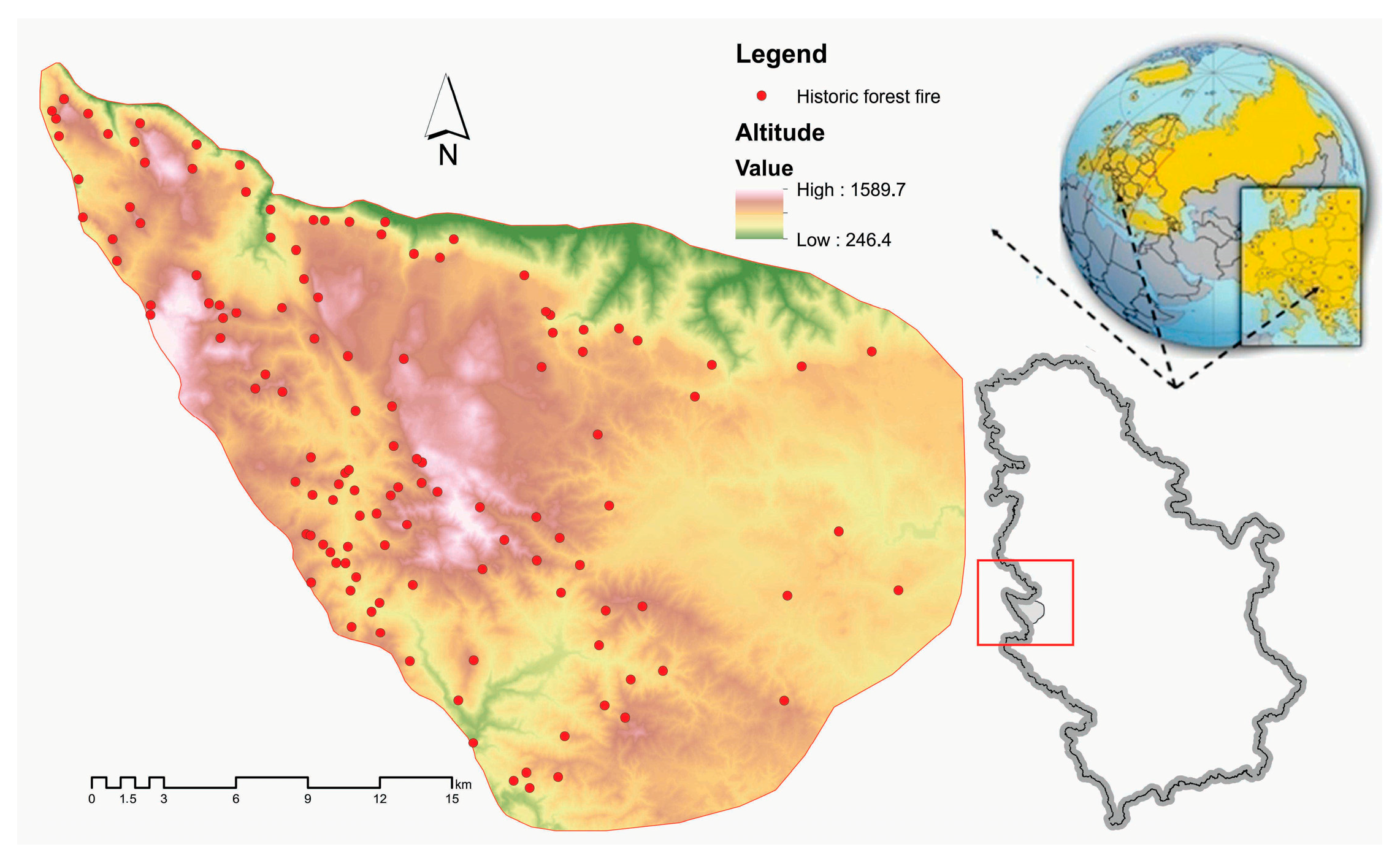
2.1. Study Area and Data
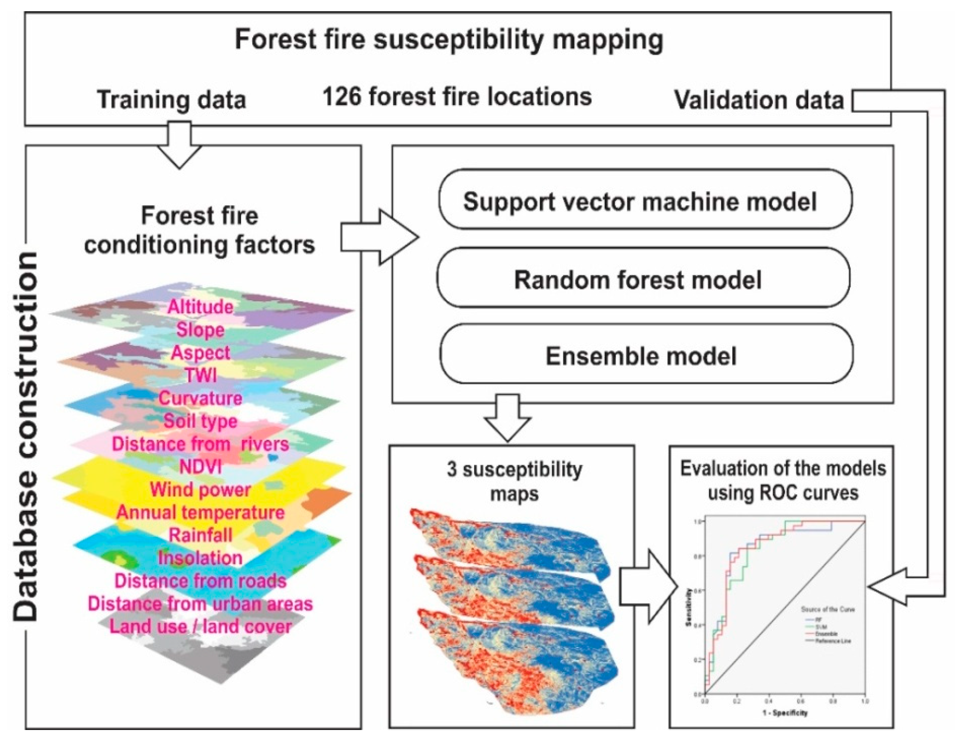
Forest area in the Republic of Serbia covers 27,200 sq. km, which is approximately 31.1% of the country area. The study area includes the whole of Serbia’s Tara National Park, which approximately covers 191.7 sq. km between latitudes of 43°43′13″ to 44°01′09″ N, and longitudes of 19°13′51″ to 19°44′20″ E. It is in the west of the Republic of Serbia (Figure 1). The study area's altitude varies from 200 to 1591 m above mean sea level (m.s.l.). Tara National Park was founded in 1981. The Tara National Park and the Mokra Gora Nature Park were nominated as potential biosphere reserves by the UNESCO MAB Committee. Mount Tara belongs to the Dinaric Alps and is part of the Old Vlach Mountains of Serbia. It is situated in the far west of Serbia, bordering the Drina River and next to the state border. Mount Tara is a medium–high mountain with an average altitude of 1000–1200 m above mean sea level (m.s.l.). The highest peak is Kozji rid at 1591 meters of altitude.
The Emerald Network program established Tara National Park as a primary butterfly area (PBA), an important bird area (IBA), and an important plant area (IPA). The Mount Tara area is a typical forest area covered by Silver Fir, European Beech, and European Spruce mixed forests (over 85% of forest area). The slope angles of the test area range from 0° to as much as 89°. The total annual rainfall ranges from 773 to 1038 mm/m2, in different parts of the study region. The maximum rainfall is between March and June, based on records from the Republic Hydrometeorological Service of Serbia.
Producing forest fire inventory maps is an important step for forest fire susceptibility mapping. The best technique for collecting data on forest fire inventory maps is still unknown. The most common is an aggregation of data collected by a combination of remote sensing technology, geographic information systems, and field work. Therefore, in this study, historical reports, field surveys, high resolution Worldview-2 images, Landsat 8 OLI and MODIS satellite images, and aerial photo interpretation were applied to prepare a forest fire inventory map. The acquisition period of satellite images for the fire inventory map is between 2010 and 2016. The analyzed aerial photos are from 2015 and 2016, with a spatial resolution of 0.4 meters. Forest fire conditioning factor is another key topic and has been researched by a lot of scientists [13,17,19,20,21,22]. Hence, different layers, including altitude, aspect, slope degree, plan curvature, topographic wetness index (TWI), normalized difference vegetation index (NDVI), distance from rivers, distance from roads, distance from urban area, annual rainfall, land use/land cover, maximum annual temperature, wind power, and soil type, have been used to analyze the forest fire susceptibility.
Topography data and digital elevation models are among the most important conditions for forest fire sensitivity mapping [13]. In the literature, such as [23,24], the impacts of aspect, altitudes, degree of slope, and curvature have been widely reported. In the current study, a digital elevation model (DEM) with 20 m spatial resolution was developed using topography data contour lines. Conditioning factors such as altitude, aspect, slope degree, plan curvature, and TWI have been created using the mentioned DEM. The land use/land cover map was created using CORINE 2006 data, whereas soil texture is extracted from national soil data. The acronym CORINE stands for Co-ORdination of INformation on the Environment, an experimental programme of the Directorate-General for Environment, Nuclear Safety and Civil protection of the Commission of the European Communities. For assessment vegetation cover, the NDVI obtained from multispectral LANDSAT 8 OLI images. The NDVI index is obtained as the mean value from the average monthly values calculated for 2016. Distance from roads, distance from rivers, and distance from urban areas were prepared using a digital topographic database at scale 1:25,000 produced in the Serbian Military Geographical Institute. Maximum annual temperature, wind power, and annual rainfall were obtained using meteorological data from the Republic Hydro-Meteorological Service of Serbia. The detailed information of data sources for forest fire conditioning factors is shown in Table 1.

2.2. Methods

The flowchart of the method used in the research is shown in Figure 2. In the first step, the data collection is presented, where all data are placed in the database. In the following, models of support vector machine, random forest, and their ensemble were applied. The validation of the constructed models was finally tested using receiver operating characteristic (ROC) curve.

3. Input Variables

3.1. Conditioning Factors

The selection of criteria for assessing the forest fire and its mapping is an important step in the analysis. To create a reliable forest fire susceptibility map, it is essential to identify forest fire conditioning factors [25]. Based on experts’ opinions and longer field observations, this study adopted fifteen criteria that are an important cause of susceptibility to forest fires in the Tara National Park of Serbia. The selected criteria with a short description are given in Table 2, and they are shown in Figure 3, Figure 4, Figure 5 and Figure 6.
In addition, a description of the soil types based on codes is shown in Table 3.
A full description of the land use/land cover conditioning factor (Figure 4d) based on codes is shown in Table 4.
Weather patterns such as temperature, rainfall, and wind power are considered as principal factors that strongly affect forest fire behavior, in which the forest fire is more likely to occur under hot, windy, and dry weather conditions. For this study, the weather data in 2016 that were available at the Republic Hydrometeorological Service of Serbia were used, including average maximum annual climatic related data: Wind power, temperature, and the total sum of rainfall (Figure 5).

3.2. Multi-Collinearity Test

In the current research, the multi-collinearity test was used to avoid the occurrence of collinearity between the conditioning factors. Multi-collinearity is a phenomenon where one predictor variable can be predicted from the other predictor variables with an extensive degree of accuracy in a multiple regression model. To quantify the severity of multi-collinearity in an ensemble learning model, tolerance and variance inflation factor (VIF) was used. Variance inflation factor contributes to a measuring index that shows how much an estimated and collinearity effected regression coefficient is increased.
A tolerance value less than 0.2 indicates multi-collinearity between independent variables, and serious multi-collinearity occurs when the tolerance values are smaller than 0.1. If the VIF value exceeds 10, it is often regarded as a multi-collinearity indication [27,28]. The tolerance and VIF values in this study are estimated and shown in Table 5. The highest VIF and the lowest tolerance were 4.496 and 0.222, respectively, based on Table 5. There is, therefore, no multi-colinearity in current research between independent factors. In the meantime, insolation had a tolerance of less than 0.1 and was removed from the following analyses.

4. Training Data Selection

In order to collect data for forest fire database, we use Moderate Resolution Imaging Spectroradiometer (MODIS), Landsat 8 OLI and Worldview-2 satellite images, extensive field surveys, and aerial photo images. In this research, a total of 126 forest fire occurrence locations were identified. Locations of forest fires are mapped and analyzed as “points”. These points refer to the points located on the center of gravity of the forest fire occurrence or centroids of the burned areas.
From a machine learning point of view of, mapping susceptibility to forest fire can be considered as a binary classification problem with two classes: Forest fire and non-forest fire. Forest fire points are coded as "1," while non-forest fire points are coded as "0" and the dependent variable is represented. For this analysis, all 126 forest fire locations were randomly divided by a random selection algorithm into two groups: Training 88 forest fire locations (70%) and validation data sets with remaining 38 forest fire hotspots (30%). The second validation dataset with the remaining 38 forest fires was used for the model validation and to confirm the prediction accuracy.
We need positive and negative examples of fire occurrence in order to build predictive models of forest fires. Positive examples were represented in the past by validation datasets of forest fire sites where we noticed the occurrence of the fire along with the date and time. The same quantity of non-forest fire points was randomly sampled from non-forest fire areas within the areas at least 15 km away from any positive example detected in timestamp ± 5 days and they represent negative examples.

5. Machine Learning Applications

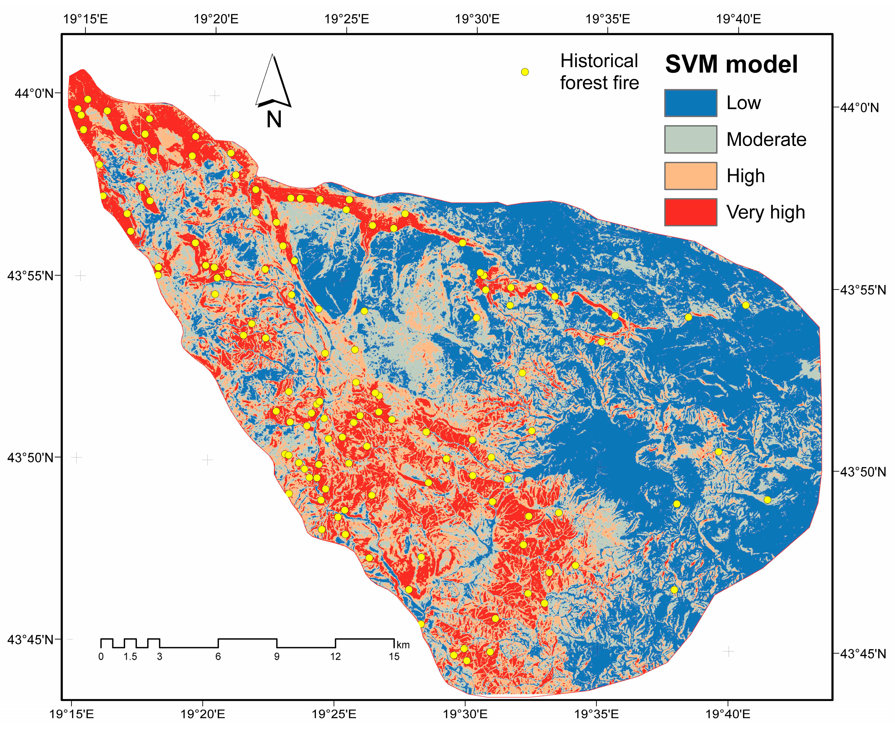
5.1. Support Vector Machine

The support vector machine (SVM) is a widely used statistical machine learning algorithm proposed by Vapnik [29] based on the basic risk minimization principle. The support vector machine algorithm separates the classes with a final surface (called an optimal hyper-plane) that optimizes the margin among the classes in the dataset. The data points of these classes closest to the hyper-plane were originally called support vectors. The main objective of SVM statistical learning algorithms is not just to separate the two classes, but also to find an optimal hyper-plane separating the two classes (i.e., wildfires and no wildfires) and the training data set.
Training data are introduced by { x i , y i } ,   i = 1 , .. r ,   y i = { 1 ,   1 } , where r is a number of training samples and the training vector consists of two classes y i = 1 for class α 1 and y i = 1 for class   α 2 . If classes are linearly separable, it is possible to define at least one hyper-plane defined by vector w with bias b, which can separate the classes properly (training error is 0) according to Equation (1):
w · x + b = 0
To find such hyper-plane, w and b are estimated in the way that y i ( w · x i + b ) 1   for   y i = 1   ( class α 1 ) and y i ( w · x i + b ) 1   for   y i = 1   ( class α 2 ) . These two can be associated based on Equation (2):
y i ( w · x i + b ) 1 0
There are many hyper-plane systems that can be used to separate two classes, but there is only one optimal hyper-plane in n dimensions. The training points closest to the optimal hyper-plane and located at the two boundaries, given with w · x i + b = ± 1 , are called support vectors and the center of the margin is the optimal hyper-plane separation.
The optimal hyper-plane between two classes is defined by maximizing the gap between the nearest classes. Mathematically, this means that we want to differentiate the two classes by their maximum distance between support vectors. This distance is equal to 2 | | w | | . This is expressed as follows:
min 1 2 | | w | | 2
subject to the following constraints:   y i ( w · x i + b ) 1 ,   where, |(|w|) | is the hyper-plane standard, b is a scalar base, and (⋅) denotes the scalar product. The cost function can be defined by using the Lagrangian multiplier as in Equation (4):
L = 1 2 | | w | | 2 i = 1 r a i ( y i ( ( w · x i ) + b ) 1 )
where, a i is the Lagrangian multiplier.
For non-linearly separable classes, the constraints can be changed by introducing slack variables ξ i [30].
Equation (3) becomes:
L = min 1 2 | | w | | 2 + C i = 1 r ξ i
where C is the constant or penalty parameter that determines the correlation between training error and the complexity of the model [31].
In order to deal with the non-linearity of the classification or regression problem, the SVM classification approach introduced certain classes of functions called kernels K ( x i , x j ) = ϕ ( x i ) ϕ ( x j ) . The original input data can easily be transferred to high-dimensional function space with certain non-linear kernel functions. The most commonly used SVM classification kernels are a radial basis function (RBF), also known as Gaussian kernels, polynomial, linear, and sigmoid kernels [29].
In this study, the radial basis function (RBF) kernel is used to model forest fire using the SVM model [32]. Since the performance of the SVM model depends on the kernel width (γ) and the regularization constant (C), they should be carefully monitored. In this research, the R open source software “rminer” package [33] was used for support vector machine modeling and optimal parameters are provided. The tuning was done in a separate data set. Features of SVM applied for forest fire modeling are:
  • SVM type applied for model: Radial Basis function.
  • Hyper-parameter: sigma = 0.054
  • Number of Support Vectors: 34
  • Objective Function Value: −93.072
  • Training error: 0.160
The best values for kernel width and regularization parameter of the SVM were obtained using the grid search method, and the optimal values were found as 0.125 and 7.95 for the kernel width and regularization parameters, respectively.
To conclude, the forest fire hazard index is symbolized with four classes using Natural Breaks classifications [31,32] and reclassified using the reclassify tool from Spatial Analyst Tools ArcGIS 10.4 software (ESRI, Redlands, California, CA, USA) release. Established on this, each cell is classified into four categories and receives a new value, low, moderate, high, or very high, representing the forest fire hazard index. The results of the forest fire susceptibility assessment using SVM model are given in Figure 7. In general, a low value is an area with the least probability of forest fire occurrence, while the very high value represents areas with the highest probability of forest fire susceptibility.

5.2. Random Forests

The random forest (RF) algorithm is an influential method of collaborative learning developed for classification, regression, and unsupervised learning [33]. Moreover, the random forest method is widely used for data prediction and is suitable for high-dimensional non-linear modeling of forest fire susceptibility. The objective of RF is to identify the appropriate model for analyzing the relationship between independent variables and a dependent variable for weight determination for each factor. In this research, training data set forest fire locations (i.e., 88 forest fire locations) and 15 forest fire conditioning factors were used as dependent and independent variables.
The RF algorithm operates by building many classification trees during the training period [34] and the final output of the model generation process is the average value of the results of all classification trees [33].
In order to run the RF model, two main parameters of the random forest model must be defined a priori: The square root of the number of factors (mtry) and the number of trees to run the model (ntree). The above parameters should be optimized to minimize the generalization error. In general, the model selects the best possible parameters for maximum accuracy [34].
Additionally, for tree learners, random forest training algorithm uses the regular technique of bagging or boot-strap aggregating. The RF method uses the Gini Index as a measure for the best split selection measuring the impurity of a given element in relation to the rest of the classes [35,36]. The Gini index is a measure of inequality of a distribution. The Gini index can be computed by summing the probability pi of a single class with label i being chosen multiplies by the probability k i p k = 1 p i   of a mistake in categorizing that class i. The Gini Index can be expressed as the following equation for a given training dataset T with j classes:
I T ( p ) = i = 1 j p i k i p k = 1 i = 1 j p i 2
where, i ∈ {1, 2, ..., j}. Therefore, a decision tree is made to grow to its maximum depth by using a given combination of features.
In this research, the RF model was used to observe the link between forest fire conditioning factors and the occurrence of forest fire and to predict the susceptibility of a forest fire. In this study, we used the Random Forest package of R open source software [36] for RF modeling and then the final produced map was added to ArcGIS 10.4 to visualize the forest fire susceptibility maps using the Spatial Analyst Tools reclassification tool. The mtry parameter was regulated using the internal random forest function. In order to obtain the values of the study area's forest fire susceptibility index, the value of each wildfire environmental factor in each grid cell was calculated using a random forest model and the parameter configuration with the highest prediction accuracy was determined and set to mtry = 5. In addition, in this study, the number of trees (mtree) in RF was fixed to 250 after a preliminary analysis and the number m of variables sampled at each node was selected to be 1. No calibration set is needed to tune the parameters. In addition, two types of error were calculated in this model: A mean decrease in accuracy and mean decrease in node impurity (mean decrease Gini). This different importance measure can be used for ranking variables and for variable selection.
The big advantage of the RF model is that it allows investigation of the variable importance (the contribution of each variable) measured by the mean reduction in prediction accuracy (Figure 8). Consequently, according to Peters [36], mean decrease in cross-validation and prediction accuracy assessment were used to examine the uncertainty propagation of conditioning factors for forest fire and to evaluate the whole random forest model.
We can see from Figure 8 that the most important conditioning factor in wildfires modeling is the slope degree, followed by NDVI, soil type, and maximum annual temperature. Namely, the fire is usually climbs uphill more easily than it descends downhill. The higher inclination effects a faster spreading of the fire [17]. Moreover, the fire follows the direction of the surrounding wind, which usually blows uphill. In addition, the smoke and heat generated by the fire, are able to heat the fuel more than the fire itself.
Using a reclassification tool in the Spatial Analyst Tools ArcGIS 10.4 software, each final map cell is classified into four categories (low, moderate, high, and very high) representing the forest fire hazard index. The obtained results of the forest fire susceptibility assessment using the random forest model are given in Figure 9. A low value (blue color) is the areas with the least probability of forest fire occurrence, while the values of very high (red color) represent areas with the highest probability of forest fire hazard.

5.3. Ensemble Modeling

Ensemble prediction is a learning algorithm that combines multiple model predictions [37] to reduce bias (boosting) and variance (bagging) or improve predictions (stacking). The Bayesian averaging is an original ensemble method, but the most popular methods for combining the predictions from different models are:
  • Boosting, which is used to build multiple models (typically the same type) using previous chain model prediction errors.
  • Bagging, which is used to create multiple models from different training dataset subsamples.
  • Stacking, which is used to build multiple models and the supervisor model that best combines the predictions of the primary models.
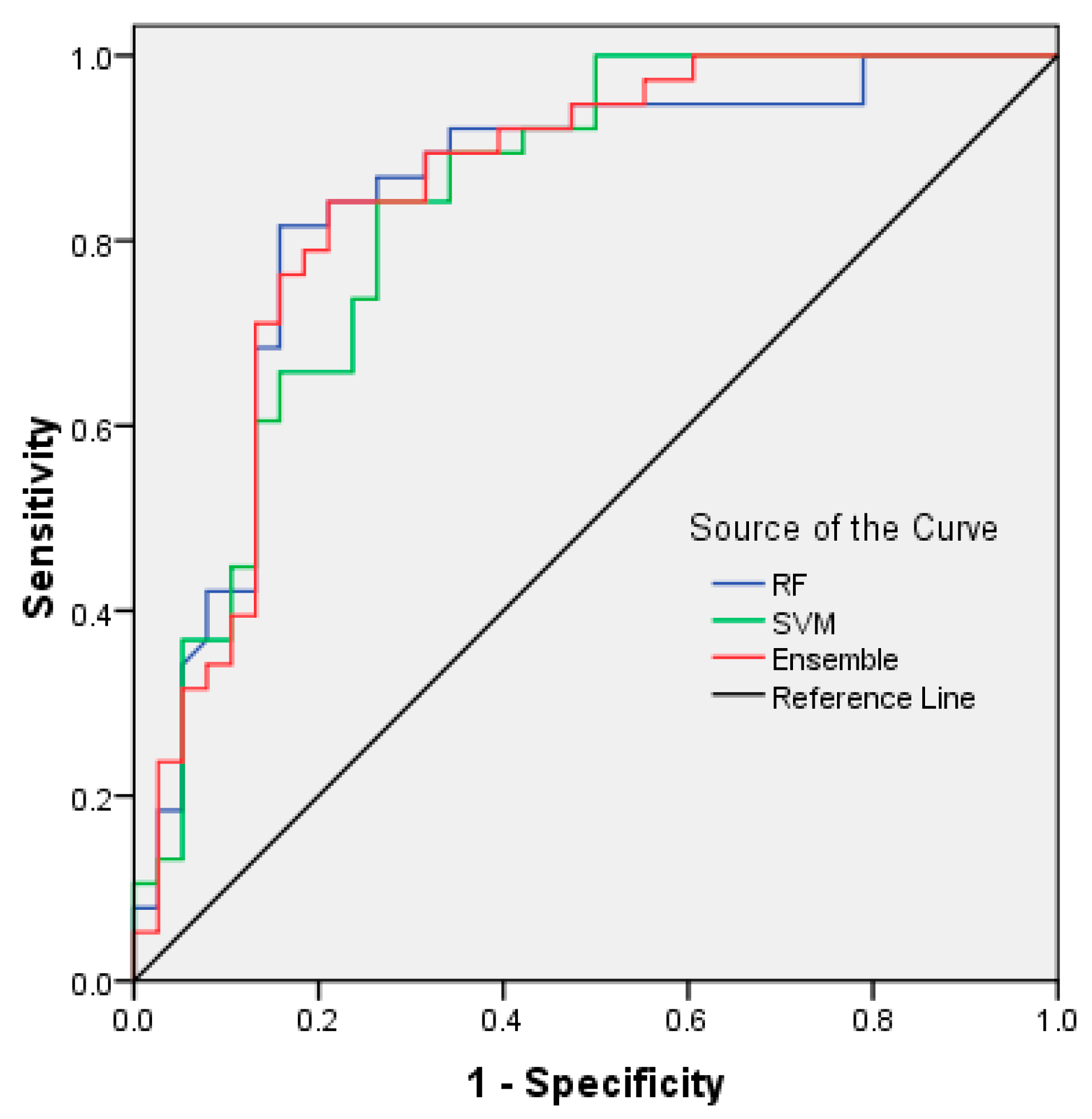
In this research, we carefully combine mentioned machine learning models to get an ensemble model using Bayesian averaging [38,39] with efficient feature selection to address these issues and mitigate their effects on the defect classification performance. Multiple predictions are made for each data point in Bayesian averaging. In this method, we take an average of predictions from all the models and use it to make the final prediction. Bayesian averaging can be used for making predictions in regression problems or while calculating probabilities for classification problems. Along with efficient feature selection, a new ensemble learning algorithm is proposed to provide robustness to both data imbalance and feature redundancy.
The achieved results of the forest fire susceptibility assessment using ensemble model are given in Figure 10. A low value (blue color) is the areas with the lowest probability of forest fire, whereas the very high values (red color) are the areas with the highest risk of a forest fire.

6. Validation

The validation of susceptibility maps for a forest fire is an important step in the modeling process. The capacity of support vector machine, random forests, and ensemble models was assessed using a non-dependent threshold approach: The operating characteristic of the receiver (ROC). The area under the curve (AUC) is a synthesized index calculated for ROC curves and it has been generally used in several types of research to assess the accuracy of the forest fire susceptibility map [40]. The AUC value is the probability that a positive event with the help of the test will be evaluated as positive. The ROC curves are generated by SPSS 17 software (IBM, New York, NY, USA) and represent the evolution of the proportion of genuine positive cases (also referred to as sensitivity) as a function of the proportion of false positive cases (corresponding to minus specificity). Graphic representation with a diagram of the pair (specificity, sensitivity) corresponds to the ROC curve for the numerous possible threshold values [41,42,43,44]. The ROC curves for SVM, RF, and Ensemble models are shown in Figure 11 and Table 6.
According to validation results, all three forest fire susceptibility maps are considered to have the most acceptable and representable appearance (AUC > 0.8). In addition, both visual assessment and quantitative validation, using ROC curve, agreed that SVM, RF, and their ensemble models are the excellent performing model approaches with an AUC value shown in Table 6.

7. Discussion

Machine learning algorithms specify computer-based tools that enable exploratory data and statistical examination to detect unknown patterns and relationships of dataset values in advance. In the current research, supervised and versatile machine learning algorithms and their ensemble were used to investigate the spatial relationship between the occurrence of forest fires and different environmental predictors [45]. The objective of this research was therefore to compare these statistical and decision tree-based regression models for forest fire mapping in the Tara National Park, Republic of Serbia. The results are presented and discussed in two important sections in the current research, including the importance of the conditioning factors and the performance of the models in the forest fire susceptibility mapping.

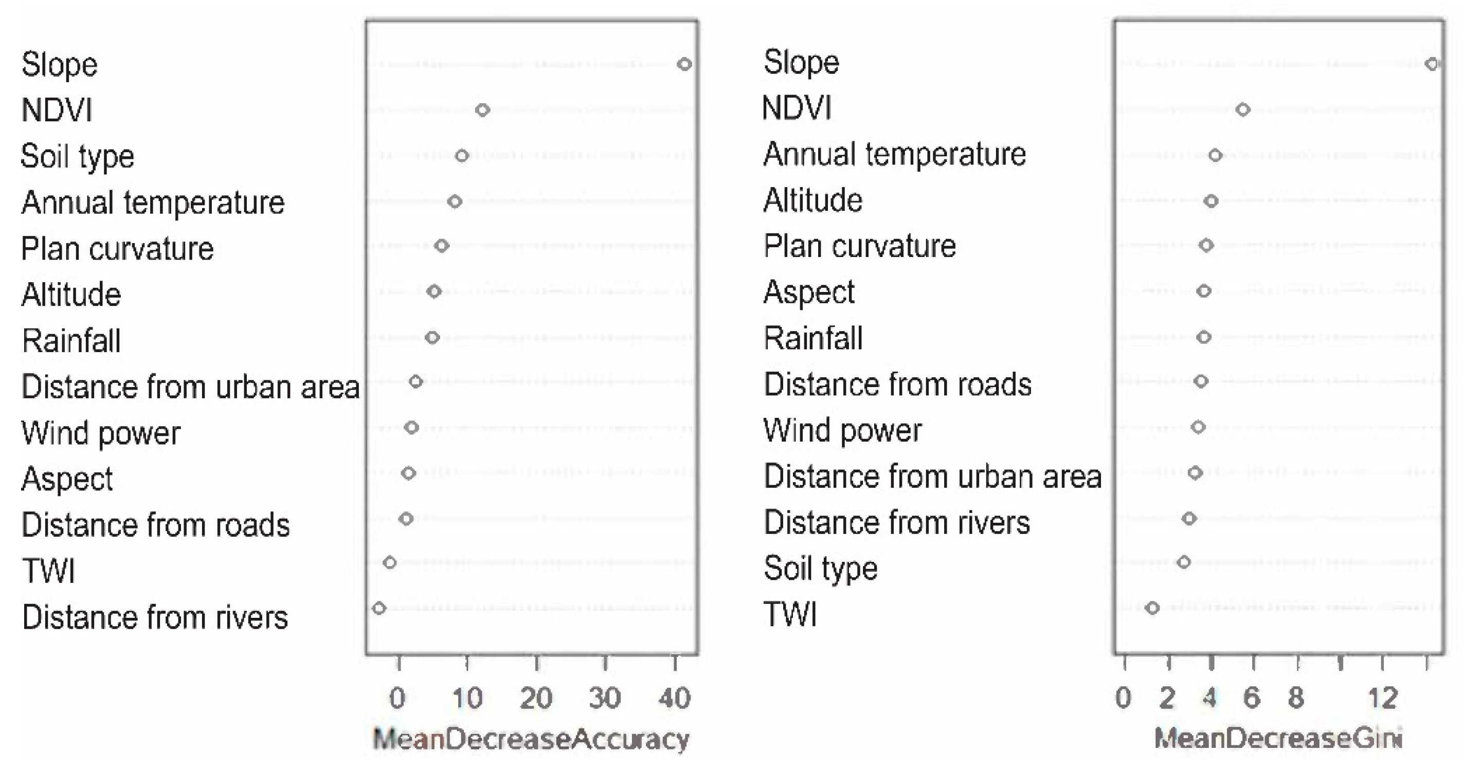
7.1. Importance of Conditioning Factors

Based on importance conditioning factor determination, the results of the current study showed that the most important conditioning factor in wildfire modeling is the slope angle, followed by NDVI, soil type, and the maximum annual temperature. Namely, the fire usually climbs uphill more easily than it descends downhill. The higher inclination effects faster spreading of the fire. On the other hand, the TWI and the distance from rivers were of the lowest importance in the occurrence of forest fires. In another study [46], slope, NDVI, and maximum annual temperature were reported to be more important in the occurrence of a forest fire, which is consistent with the results of the current research. In addition, another the research confirmed that NDVI [47], land use, soil type, and the annual temperature have a greater influence on the occurrence of the forest fire. In addition, researchers [48] found that NDVI, distance from urban areas, and distance from roads have the highest predictive values that indicate reasonable results in the forest fire susceptibility mapping.

7.2. Performance of the Used Models

The results show that the ensemble model had the highest AUC value (0.848), followed by the RF model (0.844) and the SVM model (0.834). The best performance in the current study had the ensemble method because that method combined the predictions of multiple different models together in order to decrease variance or bias and take into account advantages of both used machine learning methods. In the ensemble method, we take and use an average of predictions from all models to make the ultimate prediction. The Bayesian average can be used to predict problems of regression or to calculate probabilities of classification issues. In addition to efficient feature selection, an ensemble learning algorithm is introduced to provide robustness for both data imbalance and feature redundancy [37,48].
According to the achieved results, the support vector machine has about the same accuracy as random forest method. SVM models have produced acceptable results in the mapping of susceptibility to the forest fire. The non-linear mapping is one of the greatest advantages of the SVM model. For each class of discrete covariates, a parametric model can, therefore, have different intercepts and coefficient values. Furthermore, the SVM model is not excessively influenced by noisy data and is not very likely to overfit. The SVM model has the advantage of complex, non-linear relationships and is highly noise-resistant [49]. On the other hand, the greatest weakness of the SVM method is the fact that testing different kernel combinations and model parameters requires finding the best model. In the meantime, the results obtained are very difficult to interpret because they are part of a complex black box model.
Due to their power, versatility, and ease of use, random forests are quickly becoming one of the most popular machine learning methods. The RF performance, in the current study, being better than the SVM model could be due to its ability to run on large datasets with a large number of predictors and its ability to handle thousands of input variables without variable deletion [19]. The random forest model uses regression trees to estimate an average of the dependent variable as the final prediction results in an internally unbiased estimation of the classification error. The RF algorithm has several advantages in relation to other machine learning methods. Firstly, RF method can handle noisy or missing data as well as categorical or continuous features; secondly, it does not require assumptions about the distribution of explanatory variables; and thirdly, it can deal with interactions and non-linearities between efficient factors [50,51]. These are major advantages that limit outlier generation, particularly when working with terrain variables with a high frequency of missing data [19].
The random forests method takes advantage of the high diversity between particular trees and operates by constructing many classification trees during the training period [52]. In addition, according to Catani [52], random forests method increases variety between the classification trees by randomly changing the predictive variable sets and by resampling the data with substitution over the various tree processes of induction [17]. The result of the model construction process is the average results of all trees, so cross validation is not necessary for this method. On the other hand, the biggest weakness of RF model is the fact that, unlike a decision tree, the model is not easily interpretable. In addition, the correct use of RF model might require some work to tune the model for the data.

8. Conclusions

Many countries have detailed programs for forest fire protection, which are based on prevention and fire-fighting measures. A fire detection system is one of the most important aspects of forest fire protection before the fire spreads over larger areas. Therefore, the main purpose of this paper is to demonstrate the results of an ensemble learning method using a Bayesian average based on predictive results from the support vector machine and random forest methods. In this paper, we modeled and predicted suitable locations for the outbreak of forest fires using machine learning algorithms. Regional forest fire modeling is a regular, nonlinear and complex issue that can not be easily assessed and predicted. In the current research, we attempted to compare the results of forest fire susceptibility maps using supervised and versatile machine learning algorithms (support vector machine and random forest) and their ensemble in the Tara National Park, Serbia. Based on the obtained area under the curve, all models had the most scientifically satisfactory reliability and could be used at the regional level for forest fire susceptibility mapping. The results depicted that the ensemble model using Bayesian average had the best performance. Finally, these maps can provide very useful information for fire managers, decision makers, and foresters to locate potential fire hazard areas spatially so that they can operate under conditions in fire prevention operations in the Tara National Park of Serbia. Moreover, in national parks where the absolute priority is the preservation of natural features and endemic species, this kind of prevention from forest fires is justified and necessary. In addition, we believe that the results presented in this study make a substantial contribution to the literature on forest fire mapping.

Author Contributions

S.D. prepared the data layers, figures, and tables; H.R.P. and S.B. performed the experiments and analyses. L.G. supervised the research, finished the first draft of the manuscript, edited and reviewed the manuscript, and contributed to the model construction and verification.

Acknowledgments

This work supported research project 1.1.107/2018 "Possibilities of automatic extraction of vegetation data by a combination of satellite and aerial photogrammetric images" by the Ministry of Defence of the Republic of Serbia and research project VA/TT/3/17-19 “GIS Modeling of Risk Assessment of Disasters and Catastrophes in the Function of the Third Mission of the Army of Serbia” by the Ministry of Defense of the Republic of Serbia. This study was supported by 2015 Jiangsu provincial key R & D Program (Social Development) (BE2015704), the National Natural Science Foundation of China (No. 41877522)

Conflicts of Interest

The authors declare no conflicts of interest. The funders had no role in the design of the study, in the collection, analyses, or interpretation of data, in the writing of the manuscript, and in the decision to publish the results.

References

  1. Satir, O.; Berberoglu, S.; Donmez, C. Mapping regional forest fire probability using artificial neural network model in a Mediterranean forest ecosystem. Geomatics, Nat. Hazards Risk 2016, 7, 1645–1658. [Google Scholar] [CrossRef]
  2. Chuvieco, E.; Aguado, I.; Yebra, M.; Nieto, H.; Salas, J.; Martín, M.P.; Vilar, L.; Martínez, J.; Martín, S.; Ibarra, P.; et al. Development of a framework for fire risk assessment using remote sensing and geographic information system technologies. Ecol. Model. 2010, 221, 46–58. [Google Scholar] [CrossRef] [Green Version]
  3. Zheng, Z.; Huang, W.; Li, S.; Zeng, Y. Forest fire spread simulating model using cellular automaton with extreme learning machine. Ecol. Model. 2017, 348, 33–43. [Google Scholar] [CrossRef]
  4. Bui, D.T.; Le, K.-T.T.; Nguyen, V.C.; Le, H.D.; Revhaug, I. Tropical Forest Fire Susceptibility Mapping at the Cat Ba National Park Area, Hai Phong City, Vietnam, Using GIS-Based Kernel Logistic Regression. Remote. Sens. 2016, 8, 347. [Google Scholar] [Green Version]
  5. Wegner, J.D.; Roscher, R.; Volpi, M.; Veronesi, F. Foreword to the Special Issue on Machine Learning for Geospatial Data Analysis 2018. Available online: https://www.mdpi.com/2220-9964/7/4/147 (accessed on 24 September 2018).
  6. Pastor, E.; Zárate, L.; Planas, E.; Arnaldos, J. Mathematical models and calculation systems for the study of wildland fire behaviour. Prog. Energy Combust. Sci. 2003, 29, 139–153. [Google Scholar] [CrossRef]
  7. Andrews, P.L. BEHAVE: Fire behavior prediction and fuel modeling system-BURN Subsystem, part 1. 1986. Available online: https://www.fs.usda.gov/treesearch/pubs/29612 (accessed on 27 September 2018).
  8. Linn, R.; Reisner, J.; Colman, J.J.; Winterkamp, J. Studying wildfire behavior using FIRETEC. Int. J. Wildl. Fire 2002, 11, 233–246. [Google Scholar] [CrossRef] [Green Version]
  9. Lopes, A.M.G.; Cruz, M.G.; Viegas, D.X. FireStation — an integrated software system for the numerical simulation of fire spread on complex topography. Environ. Model. Softw. 2002, 17, 269–285. [Google Scholar] [CrossRef]
  10. Sturtevant, B.R.; Scheller, R.M.; Miranda, B.R.; Shinneman, D.; Syphard, A. Simulating dynamic and mixed-severity fire regimes: A process-based fire extension for LANDIS-II. Ecol. Model. 2009, 220, 3380–3393. [Google Scholar] [CrossRef]
  11. Perestrello De Vasconcelos, M.J.; Sllva, S.; Tome, M.; Alvim, M.; Pereira, J.M. Spatial Prediction of Fire Ignition Probabilities: Comparing Logistic Regression and Neural Networks. Photogramm. Eng. Remote Sens. 2001, 67, 73–81. [Google Scholar]
  12. Arndt, N.; Vacik, H.; Koch, V.; Arpacı, A.; Gossow, H. Modeling human-caused forest fire ignition for assessing forest fire danger in Austria. iFor. - Biogeosci. For. 2013, 6, 315–325. [Google Scholar] [CrossRef] [Green Version]
  13. Pourghasemi, H.R. GIS-based forest fire susceptibility mapping in Iran: a comparison between evidential belief function and binary logistic regression models. Scand. J. For. Res. 2016, 31, 80–98. [Google Scholar] [CrossRef]
  14. Conedera, M.; Torriani, D.; Neff, C.; Ricotta, C.; Bajocco, S.; Pezzatti, G.B. Using Monte Carlo simulations to estimate relative fire ignition danger in a low-to-medium fire-prone region. Ecol. Manag. 2011, 261, 2179–2187. [Google Scholar] [CrossRef]
  15. Amatulli, G.; Pérez-Cabello, F.; De La Riva, J. Mapping lightning/human-caused wildfires occurrence under ignition point location uncertainty. Ecol. Model. 2007, 200, 321–333. [Google Scholar] [CrossRef]
  16. Vilar, L.; Woolford, D.G.; Martell, D.L.; Martin, M.P. A model for predicting human-caused wildfire occurrence in the region of Madrid, Spain. Int. J. Wildl. Fire 2010, 19, 325–337. [Google Scholar] [CrossRef]
  17. Oliveira, S.; Oehler, F.; San-Miguel-Ayanz, J.; Camia, A.; Pereira, J.M.; Pereira, J.M.C. Modeling spatial patterns of fire occurrence in Mediterranean Europe using Multiple Regression and Random Forest. Ecol. Manag. 2012, 275, 117–129. [Google Scholar] [CrossRef]
  18. Sakr, G.E.; Elhajj, I.H.; Huijer, H.A.-S. Support Vector Machines to Define and Detect Agitation Transition. IEEE Trans. Affect. Comput. 2010, 1, 98–108. [Google Scholar] [CrossRef]
  19. Pourtaghi, Z.S.; Pourghasemi, H.R.; Aretano, R.; Semeraro, T. Investigation of general indicators influencing on forest fire and its susceptibility modeling using different data mining techniques. Ecol. Indic. 2016, 64, 72–84. [Google Scholar] [CrossRef]
  20. Arpaci, A.; Malowerschnig, B.; Sass, O.; Vacik, H. Using multi variate data mining techniques for estimating fire susceptibility of Tyrolean forests. Appl. Geogr. 2014, 53, 258–270. [Google Scholar] [CrossRef]
  21. Maeda, E.E.; Formaggio, A.R.; Shimabukuro, Y.E.; Arcoverde, G.F.B.; Hansen, M.C. Predicting forest fire in the Brazilian Amazon using MODIS imagery and artificial neural networks. Int. J. Appl. Earth Obs. Geoinformation 2009, 11, 265–272. [Google Scholar] [CrossRef]
  22. Massada, A.B.; Syphard, A.D.; Stewart, S.I.; Radeloff, V.C. Wildfire ignition-distribution modelling: A comparative study in the Huron–Manistee National Forest, Michigan, USA. Int. J. Wildl. Fire 2013, 22, 174. [Google Scholar] [CrossRef]
  23. Renard, Q.; Pélissier, R.; Ramesh, B.R.; Kodandapani, N. Environmental susceptibility model for predicting forest fire occurrence in the Western Ghats of India. Int. J. Wildl. Fire 2012, 21, 368–379. [Google Scholar] [CrossRef]
  24. Adab, H.; Kanniah, K.D.; Solaimani, K. Modeling forest fire risk in the northeast of Iran using remote sensing and GIS techniques. Nat. Hazards 2013, 65, 1723–1743. [Google Scholar] [CrossRef]
  25. Gigović, L.; Pamučar, D.; Bajić, Z.; Drobnjak, S. Application of GIS-Interval Rough AHP Methodology for Flood Hazard Mapping in Urban Areas. Water 2017, 9, 360. [Google Scholar] [CrossRef]
  26. Moore, I.D.; Grayson, R.B.; Ladson, A.R. Digital terrain modelling: A review of hydrological, geomorphological, and biological applications. Hydrol. Process. 1991, 5, 3–30. [Google Scholar] [CrossRef]
  27. O’Brien, R.M. A Caution Regarding Rules of Thumb for Variance Inflation Factors. Qual. Quant. 2007, 41, 673–690. [Google Scholar] [CrossRef]
  28. Pourghasemi, H.; Beheshtirad, M.; Pradhan, B. A comparative assessment of prediction capabilities of modified analytical hierarchy process (M-AHP) and Mamdani fuzzy logic models using Netcad-GIS for forest fire susceptibility mapping. Geomatics Nat. Hazards Risk 2016, 7, 861–885. [Google Scholar] [CrossRef]
  29. Vapnik, V.N. The Nature of Statistical Learning Theory; Springer Science & Business Media: Berlin, Germany, 1995. [Google Scholar]
  30. Foody, G.; Mathur, A. A relative evaluation of multiclass image classification by support vector machines. IEEE Trans. Geosci. Remote Sens. 2004, 42, 1335–1343. [Google Scholar] [CrossRef] [Green Version]
  31. Schölkopf, B.; Smola, A.J.; Williamson, R.C.; Bartlett, P.L. New support vector algorithms. Neural Comput. 2000, 12, 1207–1245. [Google Scholar] [CrossRef]
  32. Lee, S.; Hong, S.-M.; Jung, H.-S. A Support Vector Machine for Landslide Susceptibility Mapping in Gangwon Province, Korea. Sustainability 2017, 9, 48. [Google Scholar] [CrossRef]
  33. Liaw, A.; Wiener, M. Classification and regression by randomForest. R News 2002, 2, 18–22. [Google Scholar]
  34. Breiman, L. Random Forests. Mach. Learn. 2001, 45, 5–32. [Google Scholar] [CrossRef] [Green Version]
  35. Cutler, D.R.; Edwards Jr, T.C.; Beard, K.H.; Cutler, A.; Hess, K.T.; Gibson, J.; Lawler, J.J. Random forests for classification in ecology. Ecology 2007, 88, 2783–2792. [Google Scholar] [CrossRef]
  36. Breiman, L.; Cutler, A. Random forests — Classification description: Random forests. Available online: http//stat-www.berkeley.edu/users/breiman/RandomForests/cf_home.html (accessed on 28 September 2018).
  37. Kuhnert, P.M.; Henderson, A.; Bartley, R.; Herr, A. Incorporating uncertainty in gully erosion calculations using the random forests modelling approach. Environmetrics 2010, 21, 493–509. [Google Scholar] [CrossRef]
  38. McKay, G.; Harris, J.R. Comparison of the data-driven Random Forests model and a knowledge-driven method for mineral prospectivity mapping: a case study for gold deposits around the Huritz Group and Nueltin Suite, Nunavut, Canada. Nat. Resour. Res. 2016, 25, 125–143. [Google Scholar] [CrossRef]
  39. Dietterich, T.G. Ensemble Methods in Machine Learning. In Proceedings of the ≪UML≫ 2001—The Unified Modeling Language. Modeling Languages; Springer Nature: Berlin, Germany, 2000; pp. 1–15. [Google Scholar]
  40. Brownlee, J. Machine learning mastery. Available online: http//machinelearningmastery.com (accessed on 25 September 2018).
  41. Hoang, N.-D.; Bui, D.T. A Novel Relevance Vector Machine Classifier with Cuckoo Search Optimization for Spatial Prediction of Landslides. J. Comput. Civ. Eng. 2016, 30, 4016001. [Google Scholar] [CrossRef]
  42. Cortez, P. Data Mining with Neural Networks and Support Vector Machines Using the R/rminer Tool. In Proceedings of the ≪UML≫ 2001—The Unified Modeling Language. Modeling Languages, Concepts, and Tools; Springer Nature: Berlin, Germany, 2010; pp. 572–583. [Google Scholar]
  43. Chen, W.; Pourghasemi, H.R.; Naghibi, S.A. A comparative study of landslide susceptibility maps produced using support vector machine with different kernel functions and entropy data mining models in China. Bull. Eng. Geol. Environ. 2018, 77, 647–664. [Google Scholar] [CrossRef]
  44. Rahmati, O.; Tahmasebipour, N.; Haghizadeh, A.; Pourghasemi, H.R.; Feizizadeh, B. Evaluation of different machine learning models for predicting and mapping the susceptibility of gully erosion. Geomorphology 2017, 298, 118–137. [Google Scholar] [CrossRef]
  45. Peters, J.; De Baets, B.; Verhoest, N.E.C.; Samson, R.; Degroeve, S.; De Becker, P.; Huybrechts, W. Random forests as a tool for ecohydrological distribution modelling. Ecol. Model. 2007, 207, 304–318. [Google Scholar] [CrossRef]
  46. Hong, H.; Naghibi, S.A.; Dashtpagerdi, M.M.; Pourghasemi, H.R.; Chen, W. A comparative assessment between linear and quadratic discriminant analyses (LDA-QDA) with frequency ratio and weights-of-evidence models for forest fire susceptibility mapping in China. Arab. J. Geosci. 2017, 10, 1723. [Google Scholar] [CrossRef]
  47. Pourtaghi, Z.S.; Pourghasemi, H.R.; Rossi, M. Forest fire susceptibility mapping in the Minudasht forests, Golestan province, Iran. Environ. Earth Sci. 2014, 73, 1515–1533. [Google Scholar] [CrossRef]
  48. Bui, D.T.; Bui, Q.-T.; Nguyen, Q.-P.; Pradhan, B.; Nampak, H.; Trinh, P.T. A hybrid artificial intelligence approach using GIS-based neural-fuzzy inference system and particle swarm optimization for forest fire susceptibility modeling at a tropical area. Agric. Meteorol. 2017, 233, 32–44. [Google Scholar]
  49. Ballabio, C.; Sterlacchini, S. Support Vector Machines for Landslide Susceptibility Mapping: The Staffora River Basin Case Study, Italy. Math. For. Geosci. 2012, 44, 47–70. [Google Scholar] [CrossRef]
  50. Aertsen, W.; Kint, V.; Van Orshoven, J.; Özkan, K.; Muys, B. Comparison and ranking of different modelling techniques for prediction of site index in Mediterranean mountain forests. Ecol. Model. 2010, 221, 1119–1130. [Google Scholar] [CrossRef]
  51. Aertsen, W.; Kint, V.; Van Orshoven, J.; Muys, B. Evaluation of modelling techniques for forest site productivity prediction in contrasting ecoregions using stochastic multicriteria acceptability analysis (SMAA). Environ. Model. Softw. 2011, 26, 929–937. [Google Scholar] [CrossRef] [Green Version]
  52. Catani, F.; Lagomarsino, D.; Segoni, S.; Tofani, V. Landslide susceptibility estimation by random forests technique: sensitivity and scaling issues. Nat. Hazards Earth Syst. Sci. 2013, 13, 2815–2831. [Google Scholar] [CrossRef]
Figure 1. Location of the study area.
Forests 10 00408 g001
Figure 2. Flowchart of the forest fire susceptibility mapping.
Forests 10 00408 g002
Figure 3. Topographical factors related to forest fire; (a) altitude, (b) slope degree, (c) aspect, (d) plan curvature, and (e) topographic wetness index (TWI).
Forests 10 00408 g003
Figure 4. Environmental factors related to forest fire; (a) soil type, (b) distance from rivers, (c) normalized difference vegetation index (NDVI), and (d) land cover/land cover.
Forests 10 00408 g004
Figure 5. Meteorological factors related to a forest fire; (a) wind power, (b) maximum annual temperature, and (c) annual rainfall.
Forests 10 00408 g005
Figure 6. Social factors related to a forest fire; (a) distance from roads and (b) distance from urban areas.
Forests 10 00408 g006
Figure 7. Forest fire susceptibility map using the support vector machine model.
Forests 10 00408 g007
Figure 8. Mean decrease in prediction accuracy and mean decrease Gini index.
Forests 10 00408 g008
Figure 9. Forest fire susceptibility map using the random forest model.
Forests 10 00408 g009
Figure 10. Forest fire susceptibility map using an ensemble method.
Forests 10 00408 g010
Figure 11. Receiver operating characteristics (ROC) curves for support vector machine (SVM), random forest (RF), and ensemble models.
Forests 10 00408 g011
Table 1. Data sources and associated factor classes for forest fire susceptibility mapping.
Sub-ClassificationData LayersSource of DataGIS Data TypeDerived MapResolution
Fire Inventory DatabaseHistorical forest FireWorldview-2 images, Landsat 8 OLI images, MODIS images, aerial photo, and National fire inventory databasePoint--
TopographyElevationDEM, contour lines with 20 m intervals GRIDElevation20 m
Slope-GRIDSlope degree20 m
Aspect-GRIDAspect degree20 m
Curvature-GRIDCurvature20 m
TWI-GRIDTWI20 m
Soil typeSoilNational soil dataPolygonSoil1:50,000
Land use/land coverLand useCORINE dataARC/INFO GRIDLand use30 m
NDVINDVILandsat 8 OLI imagesARC/INFO GRIDNDVI30 m
Annual rainfallRainfallRepublic Hydro-Meteorological Service
http://www.hidmet.gov.rs/index_eng.php
GRIDPrecipitation map (mm/m2)1:50,000
Annual temperatureMax annual temperatureRepublic Hydrometeorological Service
http://www.hidmet.gov.rs/index_eng.php
GRIDTemperature map (°C)20 m
Wind powerWind powerRepublic Hydrometeorological Service
http://www.hidmet.gov.rs/index_eng.php
GRIDWind power map (m/s)20 m
RiverDrainage networkMGI Digital topographic map
http://www.vgi.mod.gov.rs/english/index_eng.html
LineDistance from rivers (m)1:25,000
RoadsRoad networkMGI Digital topographic map
http://www.vgi.mod.gov.rs/english/index_eng.html
LineDistance from roads (m)1:25,000
Urban areasUrban areasMGI Digital topographic map
http://www.vgi.mod.gov.rs/english/index_eng.html
PolygonDistance from urban areas (m)1:25,000
Table 2. Conditioning factors for forest fire susceptibility model.
CategoryDescription
Topography (Figure 3)Altitude is an important forest fire conditioning factor. An altitude map is prepared from the 20 × 20 m digital elevation model (1:25,000—scale with 20 m contour intervals).
The slope is the gradient of the land expressed as percentages or angle and it has a great influence on fir behavior. Fires burn faster on a steeped slope due to convection column flame front proximately to new fuels. Slope influences the rate of speed and fire direction.
Aspect is the direction in which a slope faces. It has an effect on the climate of the slope in terms of insolation, exposure of winds, etc. Therefore, the opposite aspect tends to retain more moisture supporting greenish and healthy vegetation.
The curvature is defined as the change rate of slope gradient or aspect, usually in a particular direction. In addition, the curvature represents convergence or divergence of water level concurrently with an activity of downhill flow. Negative, zero, and positive curvature represent concave, flat, and convex, respectively.
Topographic Wetness Index (TWI) describes the size of saturated areas of runoff generation and the effect of topography on the location. It is defined as [26]: TWI = ln (AS/tan β), where AS is the catchment area and β is the slope angle in degrees.
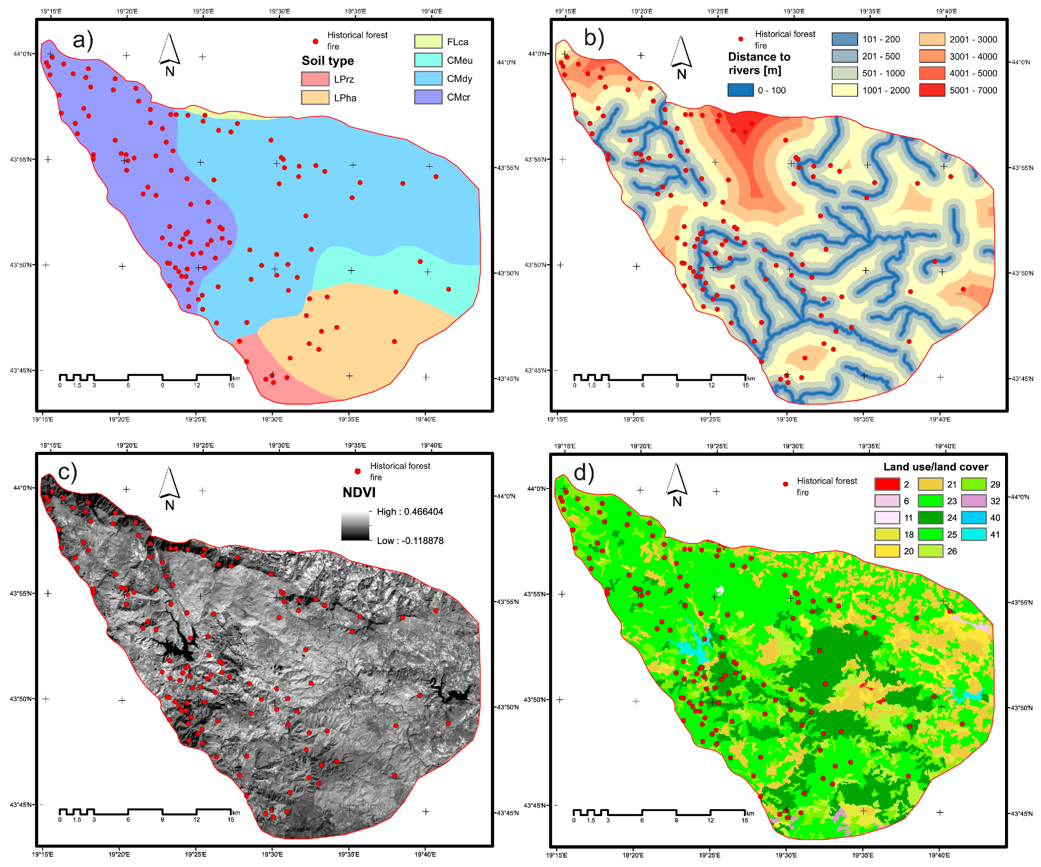
Environmental (Figure 4)Soil type reflects the affect of textures and compositions of soil materials on fire occurrence. The soil map was constructed from the soil map of the state and was classified into fine-silt, course-loamy, fine-loamy, mixed-loamy, and skeletal-loamy.
Distance from river was created using a topographical map and it was calculated based on the Euclidean distance method in ArcGIS 10.4 and were classified into (<100), (100–200), (200–500), (500–1000), (1000–2000), (2000–3000), (3000–4000), (4000-5000), and (>5000) meters classes
Normalized Difference Vegetation Index (NDVI). The NDVI map was created using multispectral Landsat 8 OLI imagery showing the surface vegetation coverage and density in an image.
Land use/land cover is considered as a factor in environmental protection. Data on land use/cover were taken on the basis of the Corine Land Cover 2006 (CLC2006) database, collected in the framework of the European Commission’s CORINE (Coordination of Information on the Environment) programme.
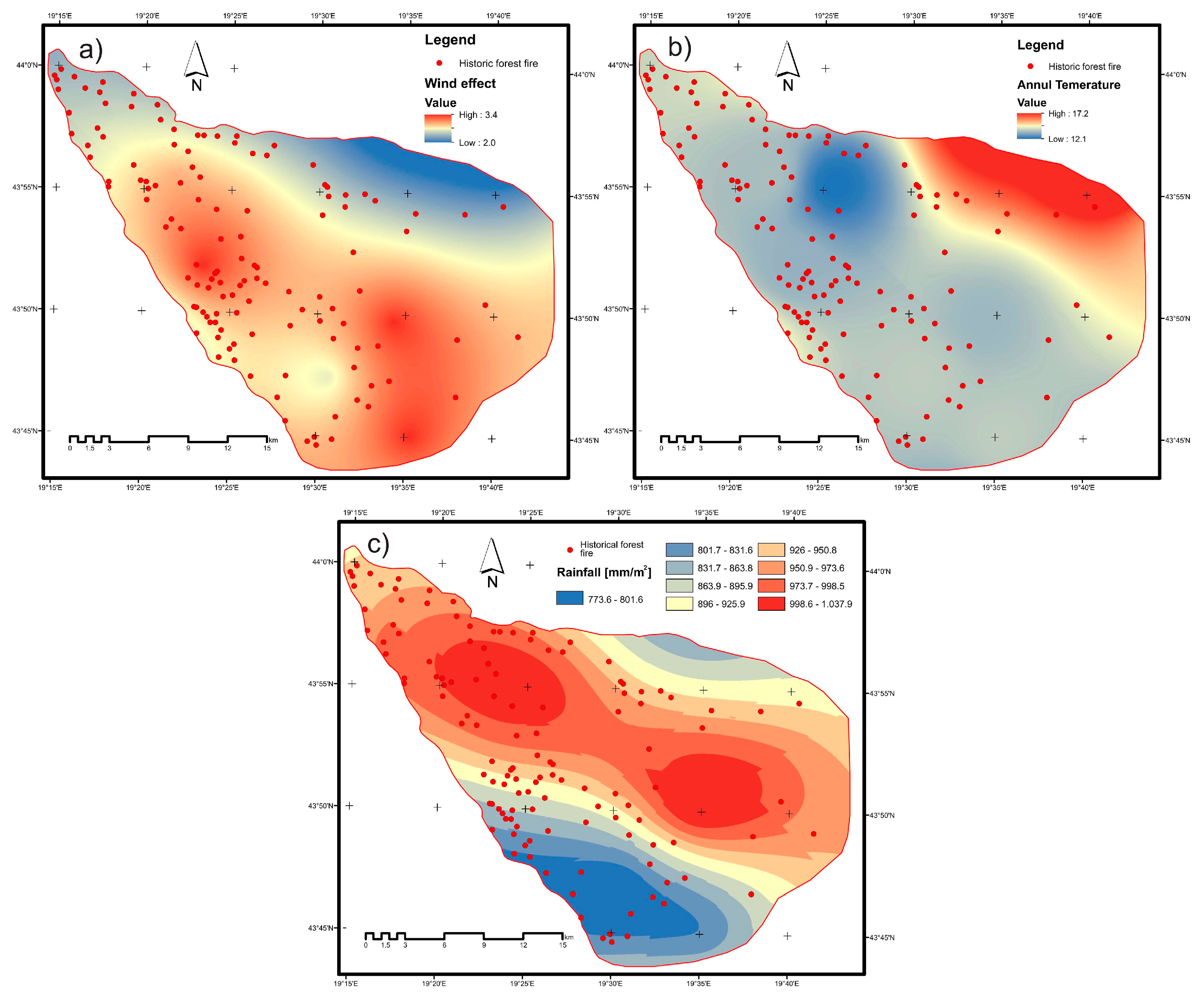
Meteorological (Figure 5)Wind power varies greatly, even at very short time scales (seconds to minutes). Two wind characteristics are used in wildfire susceptibility mapping: Wind speed and wind direction.
Annual temperature is a basic weather factor and should be taken into account. The temperature influences the condition of forest fuel, as its main effect is to dry the fuel.
Rainfall is the important effect that contributes to high fuel humidity and therefore is a negative indicator of the spread of fire. The scale was reversed to conform to the linear trend of other parameters. Annual rainfall values are divided into nine classes: (773.6–801.6, 801.7–831.6, 831.7–863.8, 863.9–895.9, 896–925.9, 926–950.8, 950.9–973.6, 973.7–998.5, 998.6–1037.9 mm/m2)
Social (Figure 6)Distance from roads was created using a topographical map, was calculated based on the Euclidean distance method in ArcGIS 10.4, and was classified into (<100), (100–200), (200-300), (300–500), (500–750), (750–1000), (1000–2000), (2000–3000), and (>3000) meters classes
Distance from urban areas was created using a topographical map, was calculated based on the Euclidean distance method in ArcGIS 10.4, and was classified into (<1000), (1000–2000), (2000–3000), (3000–4000), (4000–5000), (5000–6000), (6000–7000), and (>7000) meters classes.
Table 3. Soil type classes.
NumberCode/ValueDescription
1FlcaCalcaric Fluvisol
2CMcrChromic Cambisol
3CmdyDystric Cambisol
4CmeuEutric Cambisol
5LphaHaplic Leptosol
6LPrzRendzic Leptosol
7PldyDystric Planosol
Table 4. Land use/land cover.
NumberCode/ValueRGBCodeDescription
12255,0,0112Discontinuous urban fabric
26230,204,230124Airports
311255,230,255142Sport and leisure facilities
412255,255,168211Non-irrigated arable land
518230,230,77231Pastures
620255,230,77242Complex cultivation patterns
721230,204,77243Land principally occupied by agriculture, with significant areas of natural vegetation
823128,255,0311Broad-leaved forest
9240,166,0312Coniferous forest
102577,255,0313Mixed forest
1126204,242,77321Natural grasslands
1229166,242,0324Transitional woodland-shrub
1332204,255,204333Sparsely vegetated areas
14400,204,242511Water courses
1541128,242,230512Water bodies
Table 5. Multi-collinearity test.
ModelUnstandardized CoefficientsStandardized CoefficientsTSignificantCollinearity Statistics
BStandard ErrorBeta ToleranceVIF
(Constant)1.6741.726 0.9700.334
Aspect0.0040.0140.0210.3250.7460.9531.049
Altitude0.0000.0000.1822.0880.0380.5101.961
NDVI0.1220.6710.0140.1820.8560.6631.508
Plan curvature0.0390.0480.0520.8080.4200.9471.056
Rainfall0.0000.001−0.056−0.7000.4850.6101.640
Distance from rivers−3.372 × 10−50.000−0.072−0.9500.3440.6711.491
Distance from roads1.013 × 10−50.0000.0130.1870.8520.8251.212
Soil type0.0070.0370.0160.1840.8540.5411.850
Maximum annual temperature−0.0840.069−0.155−1.2080.2290.2344.272
Distance from urban 6.978 × 10−60.0000.0170.2330.8160.7121.404
Wind power−0.2330.236−0.130−0.9870.3250.2224.496
TWI0.0000.0080.0020.0320.9740.9421.061
Slope 0.0230.0040.5286.5030.0000.5871.704
VIF = Variance Inflation Factor.
Table 6. The area under the curve.
ModelsAreaStandard ErrorAsymptotic SignificantAsymptotic 95% Confidence Interval
Lower BoundUpper Bound
RF0.8440.0470.0010.7510.937
SVM0.8340.0470.0010.7430.926
Ensemble0.8480.0460.0010.7580.938

