Effects of Spatial Pattern of Forest Vegetation on Urban Cooling in a Compact Megacity


Abstract
1. Introduction
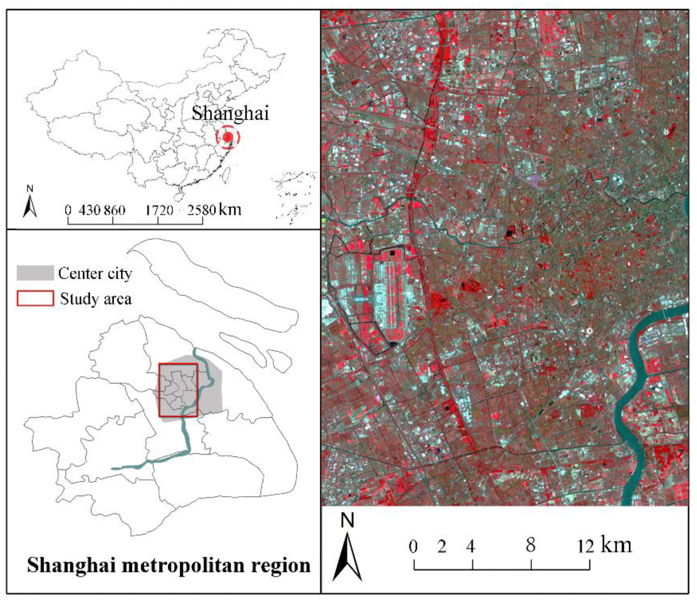
2. Study Area
3. Materials and Methods
3.1. Remote Sensing Data and the Pre-Processing
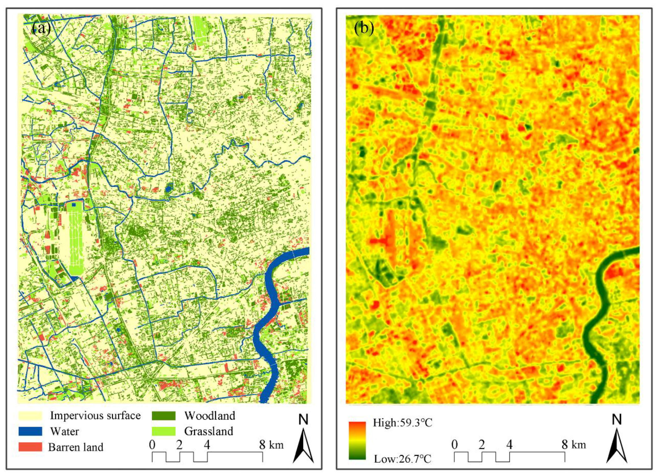
3.2. LULC Classification
3.3. Retrieval of LST
3.4. Urban Green Pattern Metrics
3.5. Moving-Window Analysis and Window Size Chosen
3.6. The Calculation of Cooling Intensity
3.7. Statistical Analysis
4. Results
4.1. The Optimal Spatial Extent for Examining the Cooling Effects of Forest Vegetation
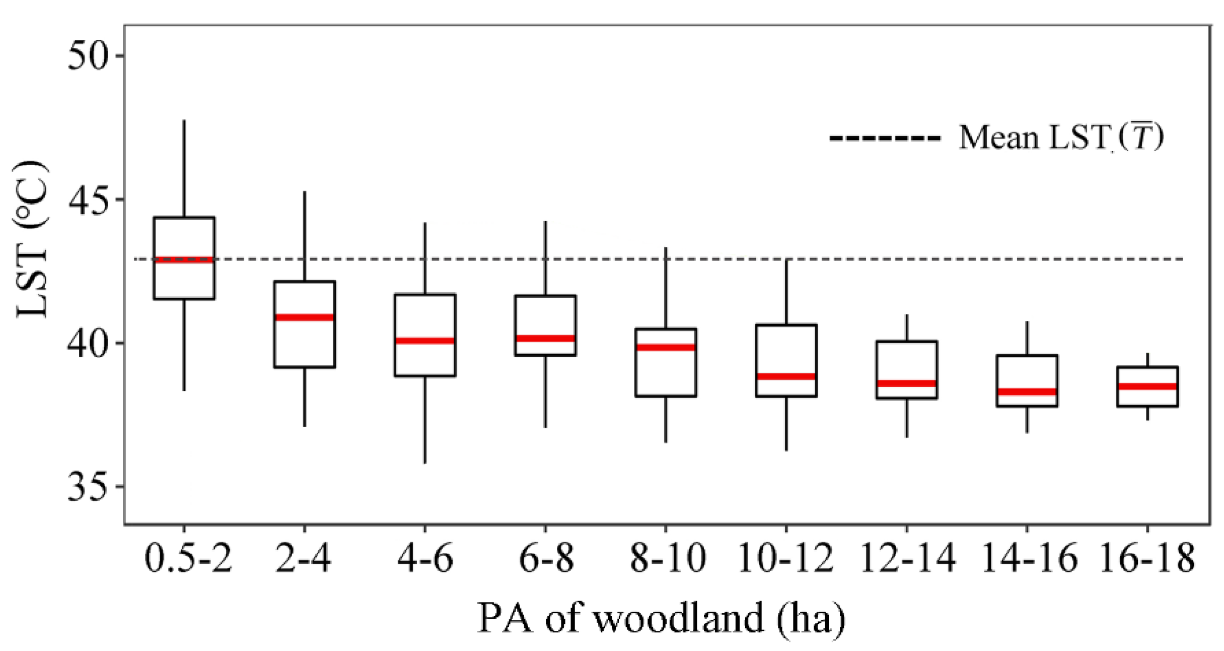
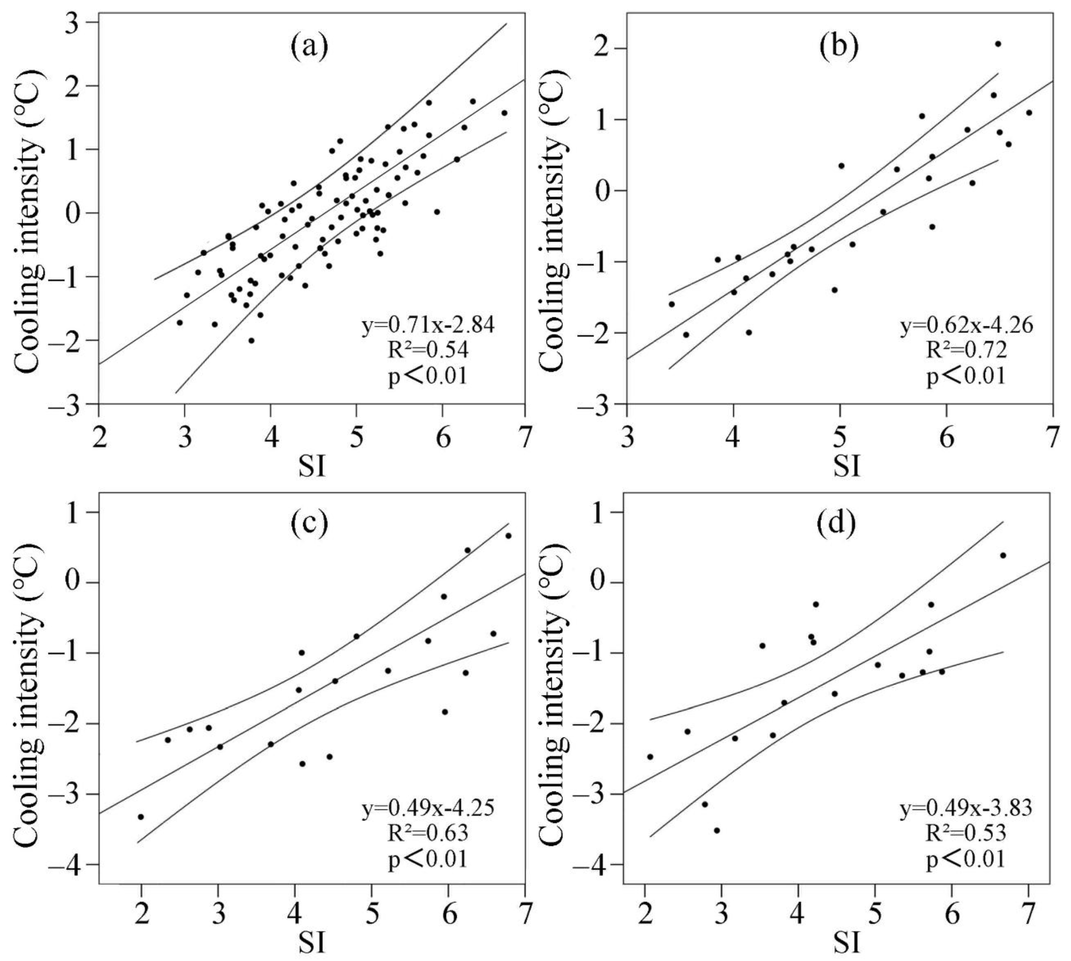
4.2. Effects of Area and Shape of Urban Woodland Patches on Cooling Intensity
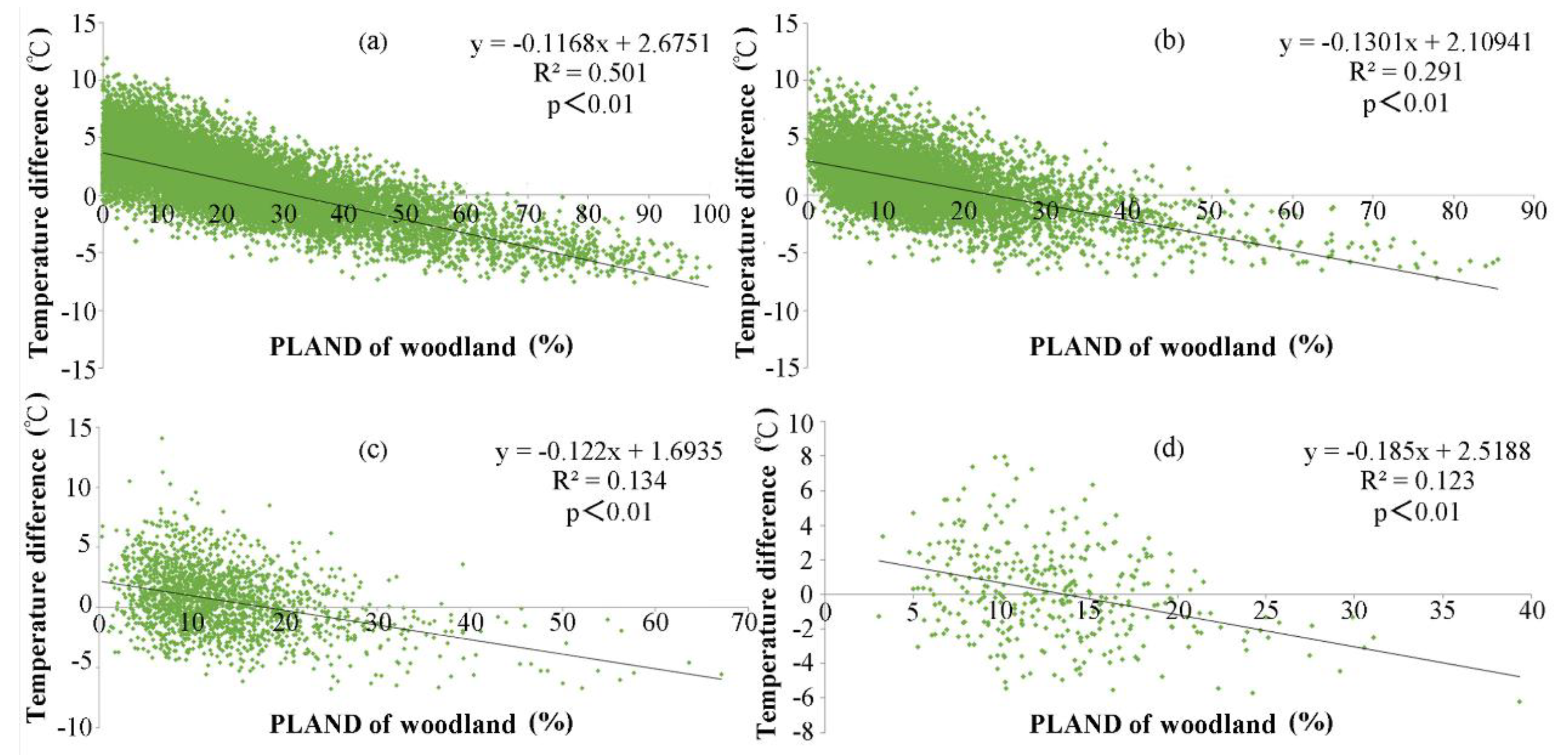
4.3. Effects of the Spatial Pattern of Vegetated Areas on Urban Cooling
5. Discussion
5.1. Implications of Optimal Spatial Extent Selection
5.2. Implications of Patch Characteristics for Forest Adaptive Planning Strategies
5.3. Implications of Spatial Patterns for Forest Adaptive Planning Strategies
6. Conclusions
Author Contributions
Funding
Conflicts of Interest
References
- United Nations, Department of Economic and Social Affairs, Population Division. World Urbanization Prospects: The 2014 Revision, CD-ROM ed.; Department of Economic and Social Affairs, Population Division: New York, NY, USA, 2014; ISBN 9789211515176. [Google Scholar]
- UNFPA. The state of the world population 2007: Unleashing the potential of urban growth. Indian Pediatr. 2008, 45, 481–482. [Google Scholar]
- Imhoff, M.L.; Zhang, P.; Wolfe, R.E.; Bounoua, L. Remote sensing of the urban heat island effect across biomes in the continental USA. Remote Sens. Environ. 2010, 114, 504–513. [Google Scholar] [CrossRef]
- Kolokotroni, M.; Ren, X.; Davies, M.; Mavrogianni, A. London’s urban heat island: Impact on current and future energy consumption in office buildings. Energy Build. 2012, 47, 302–311. [Google Scholar] [CrossRef]
- Voogt, J.A.; Oke, T.R. Thermal remote sensing of urban climates. Remote Sens. Environ. 2003, 86, 370–384. [Google Scholar] [CrossRef]
- Li, X.; Li, W.; Middel, A.; Harlan, S.L.; Brazel, A.J.; Turner, B.L. Remote sensing of the surface urban heat island and land architecture in Phoenix, Arizona: Combined effects of land composition and configuration and cadastral-demographic-economic factors. Remote Sens. Environ. 2016, 174, 233–243. [Google Scholar] [CrossRef]
- White, M.A.; Nemani, R.R.; Thornton, P.E.; Running, S.W. Satellite evidence of phenological differences between urbanized and rural areas of the eastern United States deciduous broadleaf forest. Ecosystems 2002, 5, 260–273. [Google Scholar] [CrossRef]
- Gobakis, K.; Kolokotsa, D.; Synnefa, A.; Saliari, M.; Giannopoulou, K.; Santamouris, M. Development of a model for urban heat island prediction using neural network techniques. Sustain. Cities Soc. 2011, 1, 104–115. [Google Scholar] [CrossRef]
- Santamouris, M.; Paraponiaris, K.; Mihalakakou, G. Estimating the ecological footprint of the heat island effect over Athens, Greece. Clim. Chang. 2007, 80, 265–276. [Google Scholar] [CrossRef]
- Opdam, P.; Luque, S.; Jones, K.B. Changing landscapes to accommodate for climate change impacts: A call for landscape ecology. Landsc. Ecol. 2009, 24, 715–721. [Google Scholar] [CrossRef]
- Susca, T.; Gaffin, S.R.; Dell’osso, G.R.; Dell’Osso, G.R. Positive effects of vegetation: urban heat island and green roofs. Environ. Pollut. 2011, 159, 2119–2126. [Google Scholar] [CrossRef]
- Zoulia, I.; Santamouris, M.; Dimoudi, A. Monitoring the effect of urban green areas on the heat island in Athens. Environ. Monit. Assess. 2009, 156, 275–292. [Google Scholar] [CrossRef] [PubMed]
- Bruse, M.; Fleer, H. Simulating surface-plant-air interactions inside urban environments with a three dimensional numerical model. Environ. Model. Softw. 1998, 13, 373–384. [Google Scholar] [CrossRef]
- Shashua-Bar, L.; Pearlmutter, D.; Erell, E. The cooling efficiency of urban landscape strategies in a hot dry climate. Landsc. Urban Plan. 2009, 92, 179–186. [Google Scholar] [CrossRef]
- Mackey, C.W.; Lee, X.; Smith, R.B. Remotely sensing the cooling effects of city scale efforts to reduce urban heat island. Build. Environ. 2012, 49, 348–358. [Google Scholar] [CrossRef]
- Oliveira, S.; Andrade, H.; Vaz, T. The cooling effect of green spaces as a contribution to the mitigation of urban heat: A case study in Lisbon. Build. Environ. 2011, 46, 2186–2194. [Google Scholar] [CrossRef]
- Hamada, S.; Ohta, T. Seasonal variations in the cooling effect of urban green areas on surrounding urban areas. Urban For. Urban Green. 2010, 9, 15–24. [Google Scholar] [CrossRef]
- Georgi, J.N.; Dimitriou, D. The contribution of urban green spaces to the improvement of environment in cities: Case study of Chania, Greece. Build. Environ. 2010, 45, 1401–1414. [Google Scholar] [CrossRef]
- Eliasson, I. The use of climate knowledge in urban planning. Landsc. Urban Plan. 2000, 48, 31–44. [Google Scholar] [CrossRef]
- Dimoudi, A.; Nikolopoulou, M. Vegetation in the urban environment: Microclimatic analysis and benefits. Energy Build. 2003, 35, 69–76. [Google Scholar] [CrossRef]
- Rahman, M.A.; Moser, A.; Rötzer, T.; Pauleit, S. Within canopy temperature differences and cooling ability of Tilia cordata trees grown in urban conditions. Build. Environ. 2017, 114, 118–128. [Google Scholar] [CrossRef]
- Rahman, M.A.; Armson, D.; Ennos, A.R. Effect of urbanization and climate change in the rooting zone on the growth and physiology of Pyrus calleryana. Urban For. Urban Green. 2014, 13, 325–335. [Google Scholar] [CrossRef]
- Grimmond, C.S.B.; Oke, T.R. An evapotranspiration-interception model for urban areas. Water Resour. Res. 1991, 27, 1739–1755. [Google Scholar] [CrossRef]
- Taha, H.; Akbari, H.; Rosenfeld, A.; Huang, J. Residential cooling loads and the urban heat island-the effects of albedo. Build. Environ. 1988, 23, 271–283. [Google Scholar] [CrossRef]
- Yilmaz, S.; Toy, S.; Irmak, M.A.; Yilmaz, H. Determination of climatic differences in three different land uses in the city of Erzurum, Turkey. Build. Environ. 2007, 42, 1604–1612. [Google Scholar] [CrossRef]
- Chen, A.; Yao, X.A.; Sun, R.; Chen, L. Effect of urban green patterns on surface urban cool islands and its seasonal variations. Urban For. Urban Green. 2014, 13, 646–654. [Google Scholar] [CrossRef]
- Song, J.; Li, X. A study on the cooling effects of greenery on the surrounding areas by computer simulation for green built environment. In Proceedings of the Lecture Notes in Computer Science (including subseries Lecture Notes in Artificial Intelligence and Lecture Notes in Bioinformatics), Beijing, China, 6–9 September 2010; Volume 6330, pp. 653–661. [Google Scholar]
- Bowler, D.E.; Buyung-Ali, L.; Knight, T.M.; Pullin, A.S. Urban greening to cool towns and cities: A systematic review of the empirical evidence. Landsc. Urban Plan. 2010, 97, 147–155. [Google Scholar] [CrossRef]
- Fintikakis, N.; Gaitani, N.; Santamouris, M.; Assimakopoulos, M.; Assimakopoulos, D.N.; Fintikaki, M.; Albanis, G.; Papadimitriou, K.; Chryssochoides, E.; Katopodi, K.; et al. Bioclimatic design of open public spaces in the historic centre of Tirana, Albania. Sustain. Cities Soc. 2011, 1, 54–62. [Google Scholar] [CrossRef]
- Rahman, M.A.; Armson, D.; Ennos, A.R. A comparison of the growth and cooling effectiveness of five commonly planted urban tree species. Urban Ecosyst. 2015, 18, 371–389. [Google Scholar] [CrossRef]
- Jauregui, E. Influence of a large urban park on temperature and convective precipitation in a tropical city. Energy Build. 1990, 15, 457–463. [Google Scholar] [CrossRef]
- Upmanis, H.; Eliasson, I.; Lindqvist, S. The influence of green areas on nocturnal temperatures in a high latitude city (Goteborg, Sweden). Int. J. Climatol. 1998, 18, 681–700. [Google Scholar] [CrossRef]
- Spronken-Smith, R.A.; Oke, T.R. The thermal regime of urban parks in two cities with different summer climates. Int. J. Remote Sens. 1998, 19, 2085–2104. [Google Scholar] [CrossRef]
- Kardinal Jusuf, S.; Wong, N.H.; Hagen, E.; Anggoro, R.; Hong, Y. The influence of land use on the urban heat island in Singapore. Habitat Int. 2007, 31, 232–242. [Google Scholar] [CrossRef]
- Chang, C.R.; Li, M.H.; Chang, S.D. A preliminary study on the local cool-island intensity of Taipei city parks. Landsc. Urban Plan. 2007, 80, 386–395. [Google Scholar] [CrossRef]
- Park, J.; Kim, J.H.; Lee, D.K.; Park, C.Y.; Jeong, S.G. The influence of small green space type and structure at the street level on urban heat island mitigation. Urban For. Urban Green. 2017, 21, 203–212. [Google Scholar] [CrossRef]
- Bacci, L.; Morabito, M.; Raschi, A.; Ugolini, F. Thermohygrometric Conditions of Some Urban Parks of Florence (Italy) and Their Effects on Human Well-Being. Trees 2003, 6, 49. [Google Scholar]
- Chen, Y.; Wong, N.H. Thermal benefits of city parks. Energy Build. 2006, 38, 105–120. [Google Scholar]
- Doick, K.; Hutchings, T. Air temperature regulation by urban trees and green infrastructure. For. Comm. 2013, 1–10. [Google Scholar]
- Lin, W.; Yu, T.; Chang, X.; Wu, W.; Zhang, Y. Calculating cooling extents of green parks using remote sensing: Method and test. Landsc. Urban Plan. 2015, 134, 66–75. [Google Scholar] [CrossRef]
- Tran, H.; Uchihama, D.; Ochi, S.; Yasuoka, Y. Assessment with satellite data of the urban heat island effects in Asian mega cities. Int. J. Appl. Earth Obs. Geoinf. 2006, 8, 34–48. [Google Scholar] [CrossRef]
- Schwarz, N.; Lautenbach, S.; Seppelt, R. Exploring indicators for quantifying surface urban heat islands of European cities with MODIS land surface temperatures. Remote Sens. Environ. 2011, 115, 3175–3186. [Google Scholar] [CrossRef]
- Small, C. Comparative analysis of urban reflectance and surface temperature. Remote Sens. Environ. 2006, 104, 168–189. [Google Scholar] [CrossRef]
- Chen, X.; Su, Y.; Li, D.; Huang, G.; Chen, W.; Chen, S. Study on the cooling effects of urban parks on surrounding environments using Landsat TM data: A case study in Guangzhou, southern China. Int. J. Remote Sens. 2012, 33, 5889–5914. [Google Scholar] [CrossRef]
- Schwarz, N.; Schlink, U.; Franck, U.; Großmann, K. Relationship of land surface and air temperatures and its implications for quantifying urban heat island indicators—An application for the city of Leipzig (Germany). Ecol. Indic. 2012, 18, 693–704. [Google Scholar] [CrossRef]
- Feyisa, G.L.; Dons, K.; Meilby, H. Efficiency of parks in mitigating urban heat island effect: An example from Addis Ababa. Landsc. Urban Plan. 2014, 123, 87–95. [Google Scholar] [CrossRef]
- Weng, Q. Thermal infrared remote sensing for urban climate and environmental studies: Methods, applications, and trends. ISPRS J. Photogramm. Remote Sens. 2009, 64, 335–344. [Google Scholar] [CrossRef]
- Li, Z.-L.; Tang, B.-H.; Wu, H.; Ren, H.; Yan, G.; Wan, Z.; Trigo, I.F.; Sobrino, J.A. Satellite-derived land surface temperature: Current status and perspectives. Remote Sens. Environ. 2013, 131, 14–37. [Google Scholar] [CrossRef]
- Tan, M.; Li, X. Integrated assessment of the cool island intensity of green spaces in the mega city of Beijing. Int. J. Remote Sens. 2013, 34, 3028–3043. [Google Scholar] [CrossRef]
- Keramitsoglou, I.; Kiranoudis, C.T.; Ceriola, G.; Weng, Q.; Rajasekar, U. Identification and analysis of urban surface temperature patterns in Greater Athens, Greece, using MODIS imagery. Remote Sens. Environ. 2011, 115, 3080–3090. [Google Scholar] [CrossRef]
- Cao, X.; Onishi, A.; Chen, J.; Imura, H. Quantifying the cool island intensity of urban parks using ASTER and IKONOS data. Landsc. Urban Plan. 2010, 96, 224–231. [Google Scholar] [CrossRef]
- Fan, H.Y.; Yu, Z.W.; Yang, G.Y.; Liu, T.Y. How to cool hot-humid (Asian) cities with urban trees? An optimal landscape size perspective. Agric. For. Meteorol. 2019, 265, 338–348. [Google Scholar] [CrossRef]
- Li, X.; Zhou, W.; Ouyang, Z.; Xu, W.; Zheng, H. Spatial pattern of greenspace affects land surface temperature: Evidence from the heavily urbanized Beijing metropolitan area, China. Landsc. Ecol. 2012, 27, 887–898. [Google Scholar] [CrossRef]
- Evju, M.; Sverdrup-Thygeson, A. Spatial configuration matters: A test of the habitat amount hypothesis for plants in calcareous grasslands. Landsc. Ecol. 2016, 31, 1891–1902. [Google Scholar] [CrossRef]
- Zhou, W.; Huang, G.; Cadenasso, M.L. Does spatial configuration matter? Understanding the effects of land cover pattern on land surface temperature in urban landscapes. Landsc. Urban Plan. 2011, 102, 54–63. [Google Scholar] [CrossRef]
- Weng, Q.; Lu, D.; Schubring, J. Estimation of land surface temperature-vegetation abundance relationship for urban heat island studies. Remote Sens. Environ. 2004, 89, 467–483. [Google Scholar] [CrossRef]
- Li, J.; Song, C.; Cao, L.; Zhu, F.; Meng, X.; Wu, J. Impacts of landscape structure on surface urban heat islands: A case study of Shanghai, China. Remote Sens. Environ. 2011, 115, 3249–3263. [Google Scholar] [CrossRef]
- Li, X.; Zhou, W.; Ouyang, Z. Relationship between land surface temperature and spatial pattern of greenspace: What are the effects of spatial resolution? Landsc. Urban Plan. 2013, 114, 1–8. [Google Scholar] [CrossRef]
- Liu, H.; Weng, Q.H. Scaling Effect on the Relationship between Landscape Pattern and Land Surface Temperature: A Case Study of Indianapolis, United States. Photogramm. Eng. Remote Sensing 2009, 75, 291–304. [Google Scholar] [CrossRef]
- Wu, J. Effects of changing scale on landscape pattern analysis: Scaling relations. Landsc. Ecol. 2004, 19, 125–138. [Google Scholar] [CrossRef]
- Vannier, C.; Vasseur, C.; Hubert-Moy, L.; Baudry, J. Multiscale ecological assessment of remote sensing images. Landsc. Ecol. 2011, 26, 1053–1069. [Google Scholar] [CrossRef]
- Townsend, P.A.; Lookingbill, T.R.; Kingdon, C.C.; Gardner, R.H. Spatial pattern analysis for monitoring protected areas. Remote Sens. Environ. 2009, 113, 1410–1420. [Google Scholar] [CrossRef]
- Shanghai Municipal Bureau Statistics Shanghai Statistical Yearbook 2016. Available online: www.stats-sh.gov.cn/tjnj/nj16.htm?d1=2016tjnj/C0201.htm (accessed on 30 November 2018).
- Huang, W.; Li, J.; Guo, Q.; Mansaray, L.R.; Li, X.; Huang, J. A satellite-derived climatological analysis of urban heat Island over Shanghai during 2000–2013. Remote Sens. 2017, 9, 641. [Google Scholar] [CrossRef]
- Qiu, T.; Song, C.; Li, J. Impacts of urbanization on vegetation phenology over the past three decades in Shanghai, China. Remote Sens. 2017, 9, 970. [Google Scholar] [CrossRef]
- Li, J.; Wang, X.; Wang, X.; Ma, W.; Zhang, H. Remote sensing evaluation of urban heat island and its spatial pattern of the Shanghai metropolitan area, China. Ecol. Complex. 2009, 6, 413–420. [Google Scholar] [CrossRef]
- Du, H.; Song, X.; Jiang, H.; Kan, Z.; Wang, Z.; Cai, Y. Research on the cooling island effects of water body: A case study of Shanghai, China. Ecol. Indic. 2016, 67, 31–38. [Google Scholar] [CrossRef]
- Qin, Z.; Karnieli, A.; Berliner, P. A mono-window algorithm for retrieving land surface temperature from Landsat TM data and its application to the Israel-Egypt border region. Int. J. Remote Sens. 2001, 22, 3719–3746. [Google Scholar] [CrossRef]
- McGarigal, K.; Cushman, S.A.; Neel, M.C.; Ene, E. FRAGSTATS v3: Spatial Pattern Analysis Program for Categorical Maps. Computer Software Program Produced by the Authors at the University of Massachusetts, Amherst. 2002. Available online: http://www.umass.edu/landeco/research/fragstats/fragstats.html (accessed on 25 July 2018).
- McGarigal, K.; Cushman, S.A. The gradient concept of landscape structure. In Issues and Perspectives in Landscape Ecology; Cambridge University Press: Cambridge, UK, 2005; pp. 112–119. ISBN 9780511614415. [Google Scholar]
- Beninde, J.; Veith, M.; Hochkirch, A. Biodiversity in cities needs space: A meta-analysis of factors determining intra-urban biodiversity variation. Ecol. Lett. 2015, 18, 581–592. [Google Scholar] [CrossRef]
- Klein, P.M.; Coffman, R. Establishment and performance of an experimental green roof under extreme climatic conditions. Sci. Total Environ. 2015, 512–513, 82–93. [Google Scholar] [CrossRef] [PubMed]
- Ng, E.; Chen, L.; Wang, Y.; Yuan, C. A study on the cooling effects of greening in a high-density city: An experience from Hong Kong. Build. Environ. 2012, 47, 256–271. [Google Scholar] [CrossRef]
- Rosanna, M.M.; Chapin, F.S. Urban Land Use Planning. Am. Cathol. Sociol. Rev. 2007. [Google Scholar] [CrossRef]


| Landscape Metrics | Abbreviation | Application Levels | Description | Units |
|---|---|---|---|---|
| Patch area | PA | Patch | The area of the patch | Hectares |
| Shape index | SI | Patch | The most straightforward measure of overall shape complexity | None |
| Percentage of Landscape | PLAND | Class | The proportion of total area occupied by a particular patch type; a measure of landscape composition and dominance of patch types | Percent |
| Mean patch shape index | Shape_MN | Class | Mean value of shape index of a particular patch type | None |
| Largest patch index | LPI | Class | The area (m2) of the largest patch of the corresponding patch type divided by total landscape area (m2), multiplied by 100 (to convert to a percentage) | Percent |
| Mean area | Area_MN | Class | The sum of area across all patches of the corresponding patch type divided by the number of patches of the same type | Hectares |
| Number of patches | NP | Class | The number of patches of the corresponding patch type/landscape | None |
| Aggregation index | AI | Class | The number of like adjacencies involving the corresponding class, divided by the maximum possible number of like adjacencies involving the corresponding class, which is achieved when the class is maximally clumped into a single, compact patch; multiplied by 100 (to convert to a percentage) | Percent |
| LULC Type | Mean LST | Standard Deviation of LSTs | Temperature Reduction Compared with The mean LST of Study Area | Temperature Reduction Compared with the Mean LST of Impervious Surface |
|---|---|---|---|---|
| Woodland (n = 7049) | 40.23 | 2.05 | −2.19 | −7.06 |
| Grassland (n = 4098) | 42.08 | 1.96 | −0.34 | −5.21 |
| Impervious surface (n = 2786) | 47.29 | 1.52 | 4.87 | 0 |
| Barren land (n = 495) | 43.52 | 0.89 | 1.1 | −3.77 |
| Water (n = 1250) | 37.19 | 1.01 | −5.23 | −10.1 |
| Pattern Metrics | Cooling Intensity | |||
|---|---|---|---|---|
| Pland_10 (n = 580) | Pland_20 (n = 365) | Pland_30 (n = 260) | Pland_40 (n = 190) | |
| Shape_MN | 0.38 ** | 0.23 ** | 0.45 ** | 0.39 ** |
| LPI | 0.23 ** | 0.31 ** | 0.43 ** | 0.10 * |
| Area_MN | 0.20 ** | 0.26 ** | 0.39 ** | 0.47 ** |
| NP | −0.19 ** | −0.12 * | −0.25 ** | −0.27 ** |
| AI | 0.24 ** | 0.29 ** | 0.34 ** | 0.35 ** |
© 2019 by the authors. Licensee MDPI, Basel, Switzerland. This article is an open access article distributed under the terms and conditions of the Creative Commons Attribution (CC BY) license (http://creativecommons.org/licenses/by/4.0/).
Share and Cite
Zhou, W.; Cao, F.; Wang, G. Effects of Spatial Pattern of Forest Vegetation on Urban Cooling in a Compact Megacity. Forests 2019, 10, 282. https://doi.org/10.3390/f10030282
Zhou W, Cao F, Wang G. Effects of Spatial Pattern of Forest Vegetation on Urban Cooling in a Compact Megacity. Forests. 2019; 10(3):282. https://doi.org/10.3390/f10030282
Chicago/Turabian StyleZhou, Wen, Fuliang Cao, and Guibin Wang. 2019. "Effects of Spatial Pattern of Forest Vegetation on Urban Cooling in a Compact Megacity" Forests 10, no. 3: 282. https://doi.org/10.3390/f10030282
APA StyleZhou, W., Cao, F., & Wang, G. (2019). Effects of Spatial Pattern of Forest Vegetation on Urban Cooling in a Compact Megacity. Forests, 10(3), 282. https://doi.org/10.3390/f10030282