Article

Spatiotemporal Ozone Level Variation in Urban Forests in Shenzhen, China

1
Research Institute of Forestry, Chinese Academy of Forestry/Urban Forest Research Center, State Forestry and Grassland Administration/Key Laboratory of Forest Silviculture of State Forestry and Grassland Administration, Research Institute of Forestry, Chinese Academy of Forestry, Beijing 100091, China
2
Research Institute of Tropical Forestry, Chinese Academy of Forestry, Guangzhou 510520, China
*
Author to whom correspondence should be addressed.
Forests 2019, 10(3), 247; https://doi.org/10.3390/f10030247
Submission received: 6 January 2019 / Revised: 4 March 2019 / Accepted: 6 March 2019 / Published: 11 March 2019
(This article belongs to the Section Forest Ecology and Management)

Abstract

:
This study is among the first to investigate ozone levels in urban forests in China. It establishes that urban forest air quality in Yuanshan Forest Park (Shenzhen) is suitable for recreational activities and identifies spatial, seasonal, and diurnal O3 patterns and relationships with micrometeorological parameters, suggesting the possibility of manipulating relevant forest characteristics to reduce Surface ozone (O3) levels. An understanding of O3 levels of urban forest environments is needed to assess potential effects on human health and recreational activities. Such studies in China are scarce. This study investigated urban forest O3 levels to improve understanding and support residents engaging in forest recreational activities. We monitored O3 levels in 2015–2016 for three urban forests representing common habitats (foothill, valley, and ridge) in Yuanshan Forest Park and for an adjacent square. The overall mean daily and daily maximum 8 h mean (MDA8) O3 concentrations were highest for the ridge forest and lowest for the valley forest. Each forest’s O3 concentrations were highest in summer. Diurnally, forest O3 concentrations peaked between 13:00 and 17:00 and reached a minimum between 03:00 and 09:00. The correlation between forest O3 concentrations and air temperature (AT) was strongly positive in summer and autumn but negative in spring. In each season, O3 concentration was negatively correlated with relative humidity (RH). No MDA8 or hourly O3 concentrations in the forests exceeded National Ambient Air Quality Standard Grade I thresholds (100 and 160 μg m−3, respectively). O3 accumulation is present in ridge urban forest in all seasons. Foothill and valley urban forests have better air quality than ridge forestation. Urban forest air quality is better in spring and autumn than in summer and is better from night-time to early morning than from noon to afternoon.

1. Introduction

With the acceleration of urbanization in China, the construction of urban forests has increased and the area covered by urban forest has been expanding, especially in metropolitan areas. Urban forests can provide a high-quality environment that includes clean air, a comfortable microclimate, low noise, and high biodiversity, which benefit physical and mental health [1,2]. An increasing number of urban citizens visit urban forests for leisure and for recreational or fitness activities such as walking or running, requiring close monitoring of the air quality of urban forests [3,4,5].
Surface ozone (O3) is a main secondary gaseous pollutant in urban areas; it forms in reactions in which volatile organic compounds (VOCs) interact with NOx in the presence of sunlight [6,7,8]. Numerous medical studies have demonstrated that high levels of O3 can affect human health. For instance, it can increase the frequency of occurrence of lung disease and mortality in urban inhabitants under long-term exposure [9,10,11,12,13]. Thus, O3 levels are an important indicator of air quality and elevated O3 levels in the urban environment require a deeper understanding of O3 levels in urban forests to help residents engage in healthful recreational and fitness activities.
Most previous studies conducting modelling-based evaluation, such as observations of 86 cities in Canada, 10 metropolitan cities in Italy, and areas in Florence (Italy) and Strasbourg (France) [14,15,16,17], demonstrated that urban forests are capable of reducing O3 levels. In addition, studies using sap flow measurements and eddy covariance systems to investigate the effect of urban trees on O3 showed that urban trees can remove O3 though the canopy stomata uptake and non-stomatal deposition [18,19,20].
Some recent studies have focused on biogenic emissions from urban forests and their effects on O3 levels. Results from these studies indicate that urban trees can increase O3 concentrations by emitting a variety of O3 precursors—e.g., biogenic volatile organic compounds (BVOCs) such as isoprene and (mono)terpenes, which are estimated to be two to three times more photochemically reactive than hydrocarbons of anthropogenic origin—and different plant species feature different O3 formation potential [7,21,22]. Thus, existing research on the effects of urban forest on O3 provides contradictory results.
Most investigations conducted in China focus on the toxic effects of O3 on plants [23,24,25] or the contribution of BVOCs emitted from trees to O3 formation [26,27], whereas O3 levels in urban forests have rarely been characterized. Herein, in order to improve the understanding of the O3 level in urban forests as well as to help residents engage in more healthful forest recreational activities, we empirically characterize O3 levels measured in 2015–2016 for (a) three types of forest representing common habitats in Yuanshan Forest Park (Shenzhen) and (b) an adjacent square with little vegetation. Additionally, the micrometeorological parameters of air temperature (AT), relative humidity (RH), wind speed (WS), and solar radiation (SR) were monitored simultaneously with O3 concentration at each site. The objective of this study was to (1) understand the effect of urban forest on O3 levels, (2) investigate O3 level dynamics in urban forests and the best time for residents to engage in recreation, and (3) explore the effects of micrometeorological parameters on O3 levels in urban forests.

2. Materials and Methods
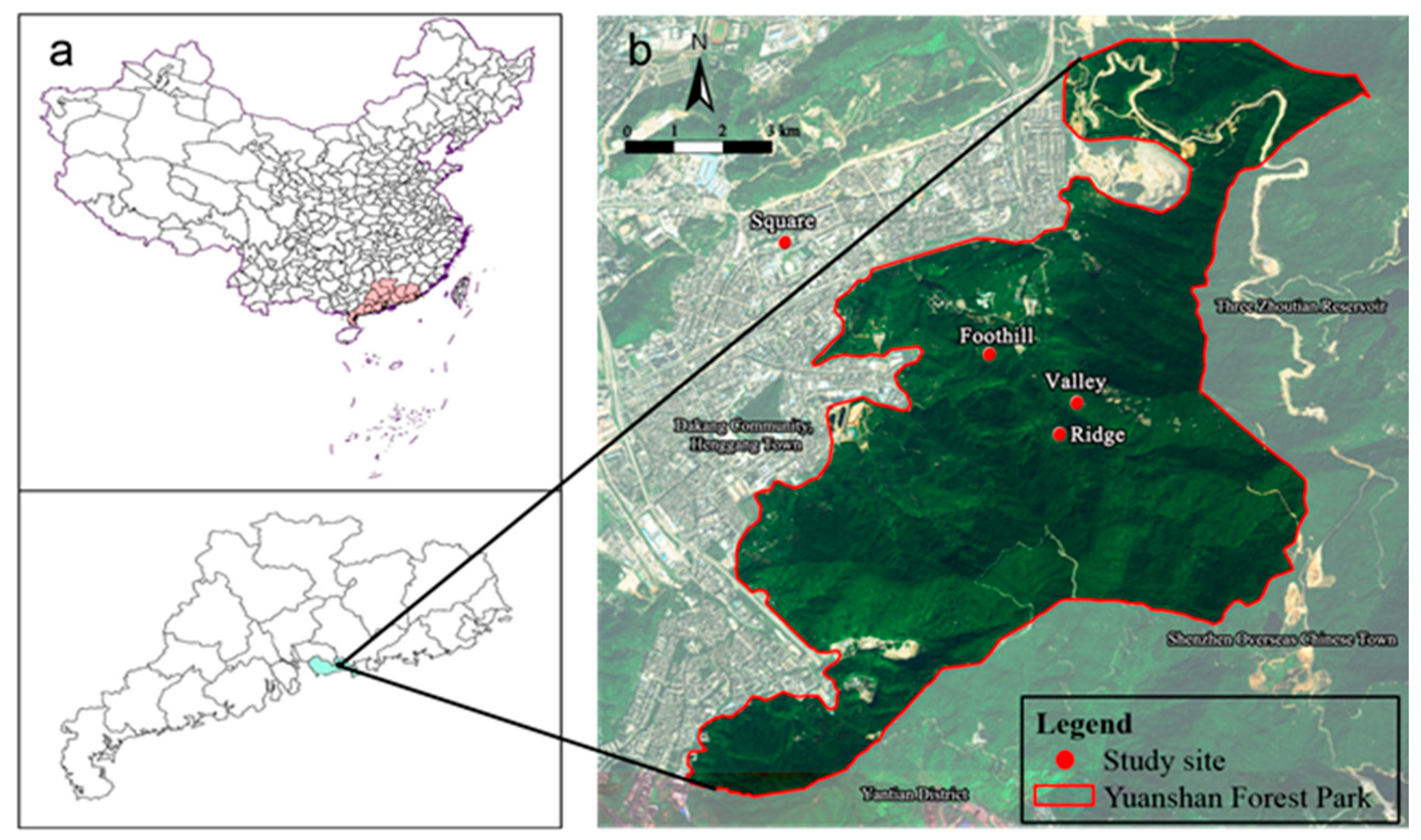
2.1. Study Area

The study area was located in Shenzhen, Guangdong Province, in southern China. During the past 20 years, Shenzhen has become one of the most prosperous cities in China, having a residential population of over 10 million in 2015 (Shenzhen Statistics and Information Bureau, 2015) and covering an area of 1996.85 km2, with urban forests currently accounting for more than 60% of the green space.
The primary terrain of Shenzhen consists of rolling hills; it also features some low mountains and coastal plains. The climate is dominated by the southern subtropical ocean monsoon. The precipitation period is from April to September and vegetation is largely represented by secondary forests and plantations of southern subtropical evergreen broadleaf forests, with the most common plants including Acacia mangium and those of the Eucalypteae tribe [28].
For this study, field measurements were performed in Yuanshan Forest Park, which is located in eastern Shenzhen at a distance of 20 km from the city centre and which has become an important locale for recreational activities of nearby residents. The park area totals ~10.9 km2 and the elevation ranges from 60 to 599 m. Importantly, no industrial or traffic facilities are located within the park and more than 85% of its area is covered by vegetation (mainly evergreen broadleaf forest).

2.2. Monitoring Sites

For systematically characterizing O3 levels in urban forest, three types of forest—located in the foothills, in the valley, and on the ridge of the main peak in Yuanshan Forest Park—were selected as monitoring sites. Each area had a size of no less than 600 m2, featured a gentle slope (≤35°), and was suitable for recreation. An aerial photograph of the study area and monitoring sites is shown in Figure 1.
Each site comprised six monitoring points located 30 m from the forest margin and situated under the canopies of trees similar in size. Thus, a total of 18 monitoring points was established in the three forests. The distance between any two points was set to a minimum of 50 m to allow good exposure to the surrounding environment.
In addition, a square with little vegetation which is about 2.1 km away from the park was used for comparison. This plot (50 × 50 m) was located in a residential area surrounded by a low-traffic road and low-rise buildings and therefore had an environment similar to that of the park except with less vegetation. Six monitoring points were set in the square using the same criteria described above.

2.3. Monitoring Methods and Dates

O3 concentrations were monitored using 24 portable O3 monitors (Aeroqual Series 500, Auckland, New Zealand) having a detection range of 0–1000 µg m−3, a resolution of 2 µg m−3, and an accuracy of within ± 16 µg m−3 from 0 to 200 µg m−3 and ± 20 µg m−3 from 200 to 1000 µg m−3 [29,30]. The monitor had proven to be reliable and accurate in numerous previous studies [31,32,33]. Micrometeorological parameters (AT, RH, WS, and SR) were monitored using a pocket weather station (Kestrel 5500, Nielsen-Kellerman, Boothwyn, PA, USA) and a digital luminance meter (TES-1332A, TES Electrical Electronic Corp., Taipei, Taiwan). O3 concentrations and micrometeorological parameters were measured at an elevation of ~1.5 m above ground, which is commonly considered the typical height at which human respiration occurs. All metrics were observed manually, and one observer was established at each point, for a total of 24 observers. Monitoring was nominally performed for 24 h each day (from 09:00 to 09:00 of the following day) at 2 h intervals. Sampling was performed 30 min each time and data were automatically recorded by an internal memory logger, stored on the monitor, and converted into hourly averages at each point. The metrics were monitored simultaneously at the same times for all points.
Observations were conducted in three different months, representing three different seasons: April 2016, spring; August 2015, summer; January 2016, autumn (April 2016, spring; August 2015, summer; January 2016, autumn). For each season, six sunny days were selected for monitoring.

2.4. Vegetation

To understand the vegetation composition of three urban forests, surveying was performed in November and December 2015 within a 30 × 40 m plot in each experimental forest, and all trees and tall shrubs with a diameter at breast height (DBH) of >2 cm were recorded. For trees, five variables were collected (canopy cover, species, number, height, DBH), and dominant species were determined according to the method of Wang et al. [34]. The main plant species in the three forest plots are listed in Table 1.

2.5. Data Analysis

To determine and compare the effect of urban forests on O3 levels, we averaged the values for the daily concentrations of O3 supplied by the Meteorological Bureau of Shenzhen Municipality and the Shenzhen Environmental Monitoring Centre Station for each monitoring period and used them as the background data for the city of Shenzhen. There were 11 background stations including Honghu station (urban site, located 14.3 km southwest of the park), Overseas Chinese Town station (urban site, located 28.8 km southwest of the park), Yantian station (urban site, located 34.2 km west of the park), Longgang station (urban site, located 9.6 km north of the park), Xixiang station (suburban site, located 36.6 km west of the park), Nanao station (suburban site, located 27.7 km southeast of the park), Kuiyong station (suburban site, located 19.6 km east of the park), Meisha station (suburban site, located 8.6 km southeast of the park), Guanlan station (urban site, located 19.6 km northwest of the park), Tongxinlingzi (urban site, located 19.1 km southwest of the park), and Nanhaizi station (suburban site, located 28.8 km w of the park), all of which were over 15 km far from Yuanshan Forest Park. The daily (from 01:00 to 01:00 of the following day) means of O3 concentration of urban forests were calculated to compare with daily data from background stations. In addition, the O3 levels in the urban forests were compared to the Grades I and II hourly and daily maximum 8 h (11:00–18:59) mean (MDA8) concentrations of O3 stipulated by the National Ambient Air Quality Standard (NAAQS Grade I: 160 and 100 µg m−3; Grade II: 200 and 160 µg m−3, respectively).
One-way analysis of variance (ANOVA) and Duncan’s test were used to determine the significance of differences between the overall daily average O3 concentrations at different sites. Two-way ANOVA and Duncan’s test were used to compare the differences of daily mean concentrations of O3 between different seasons and sites. The Pearson correlation test was applied to detect possible correlations between O3 and micrometeorological parameters. For all tests, p values of <0.05 were considered to represent statistical significance. Statistical analyses were performed using SPSS Statistics, Version 22 (SPSS Inc., Chicago, IL, USA). Plots were created in Origin 9.0 (OriginLab, Hampton, NH, USA). Tables were prepared using Microsoft Excel 2016 (Microsoft, Redmond, WA, USA).

3. Results

3.1. O3 Concentration

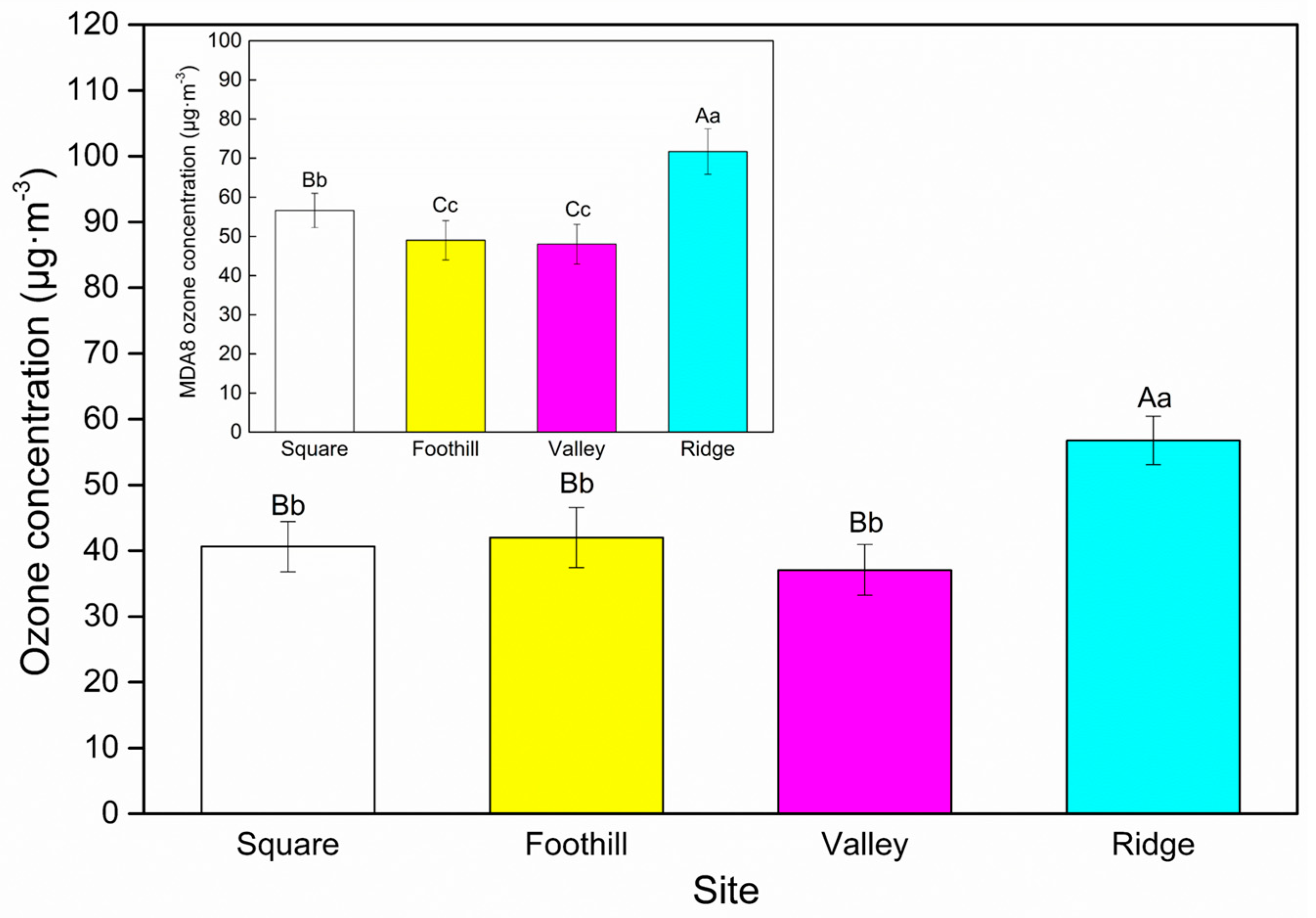
3.1.1. Overall Characteristics

The overall mean daily O3 concentration ([O3]DA) was highest for the ridge forestation and lowest for the valley forestation (Figure 2). Notably, the [O3]DA of the ridge forestation was significantly higher than that of the square (by 39.76%). In addition, the [O3]DA of the ridge forestation was insignificantly (1.06-fold) higher than the background value (53.44 ± 4.17 μg m−3; not shown in the figure), whereas the values for the foothill and valley forestation were significantly lower (by 27.18% and 44.12%, respectively).
The MDA8 O3 concentration ([O3]MDA8) values for ridge forestation were significantly higher than those for the square (by 26.62%), whereas the corresponding values for foothill and valley forestation were significantly lower than those for the square (by 15.53% and 17.91%, respectively). In addition, the [O3]MDA8 values for the three forests did not exceed the NAAQS Grade I (GB3095-2012) threshold of 100 μg m−3 for O3, which was set for clean-air areas such as scenic spots and represents a level that has no effect on human health.

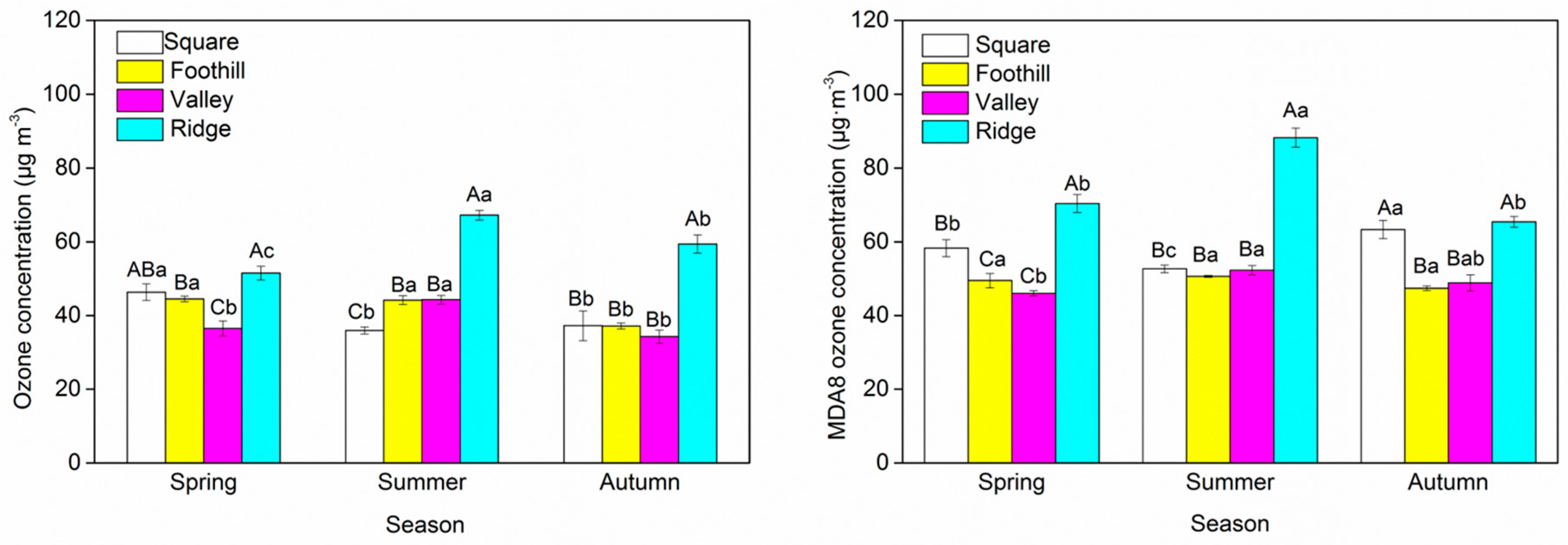
3.1.2. Seasonal Variation

For all forest sites, the highest [O3]DA and [O3]MDA8 values generally appeared in summer, whereas for the square, the summer values of [O3]DA and [O3]MDA8 were the lowest (Figure 3), in agreement with the background values of [O3]DA (70.67, 57.00, and 32.67 μg m−3 for spring, autumn, and summer, respectively; not shown in the figure).
For each season, the highest [O3]DA and [O3]MDA8 values were observed for the ridge forestation, whereas the lowest values were observed for the foothill or valley forestation except in summer. In spring, the [O3]DA values for the four sites were significantly lower than background values (not shown in the figure) by >30%. In summer, the [O3]DA values for the three forest sites were significantly higher than those for the square and the background values (not shown in the figure) by 22.82–86.83% and 35.26–105.75%, respectively. In autumn, the [O3]DA values for the foothill and valley forestation were close to that of the square and were significantly lower than the background value (not shown in the figure) by >34.50%, whereas the corresponding [O3]MDA8 values were lower than that of the square by 20.93% and 18.56%, respectively. In each season, the [O3]MDA8 values for the three forest sites did not exceed the NAAQS Grade I threshold of 100 μg m−3 for O3, but the summer attainment efficiency for the ridge forestation was only 11.79%.

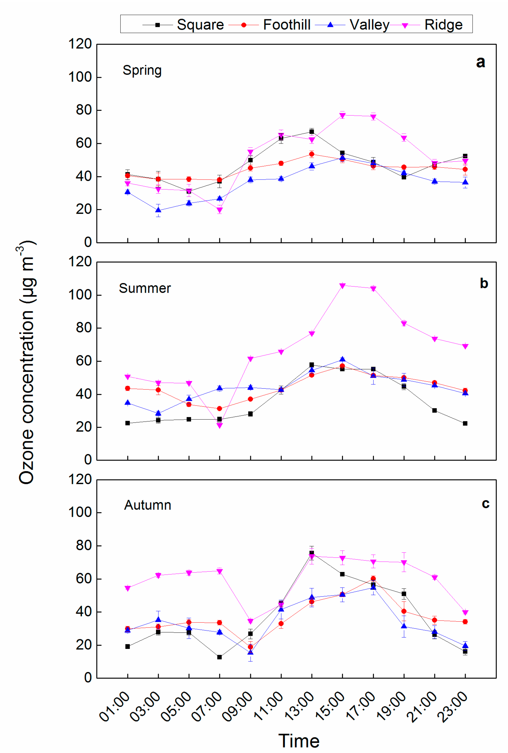
3.1.3. Diurnal Variation

The average diurnal cycles of O3 concentration for all sites were similar in each season (Figure 4). In spring, the O3 concentration was generally minimal between 03:00 and 07:00, rapidly increasing to reach a noon-to-afternoon maximum between 13:00 and 17:00 and then stably decreasing during evening hours (Figure 4a). However, the curve’s shape is strongly site-dependent. For example, a steep plateau and the highest daily variation (57.19 μg m−3) was observed for the ridge forestation, thus flatter shapes were observed in cases of lower daily variation for foothill and valley forestation and for the square (36.04, 31.83, and 15.44 μg m−3, respectively).
In summer, the mean diurnal cycles for all sites were consistent with those observed in spring (Figure 4b). The largest daily variation observed for the ridge forestation (84.58 μg m−3) was significantly (1.38-fold) higher than that of the square, whereas a smaller value was observed for the valley forestation (32.7 μg m−3, close to that of the square), and the smallest variation was observed for the foothill forestation (25.94 μg m−3).
In autumn, the mean diurnal cycles for all sites featured a small flat plateau from 01:00 to 07:00 followed by a sharp decrease to a morning (07:00–09:00) minimum and a later rapid rise to an afternoon (13:00–17:00) maximum (Figure 4c). The largest daily variation was observed for the square and significantly smaller values were observed for the three forest sites (decreases of 34.20–37.85%). In addition, none of the hourly O3 concentrations in the three types of urban forest exceeded the NAAQS Grade I threshold of 160 μg m−3 in any season and the attainment efficiency exceeded 34%. Thus, the ozone levels in the three types of urban forest in Yuanshan Forest Park did not reach the level of harm to human health and ranged within the clean level, which is in line with the requirements for air quality of the environment for residents’ forest recreation.
For a specific site, the daily variation varied from season to season. For foothill and valley forestation, the daily variation was largest in autumn and smallest in spring. For ridge forestation, the daily variation in summer significantly exceeded those for spring and autumn (by 47.89% and 116.76%, respectively). However, for the square, the daily variation in autumn was significantly higher (by ~75%) than those determined for the other two seasons.

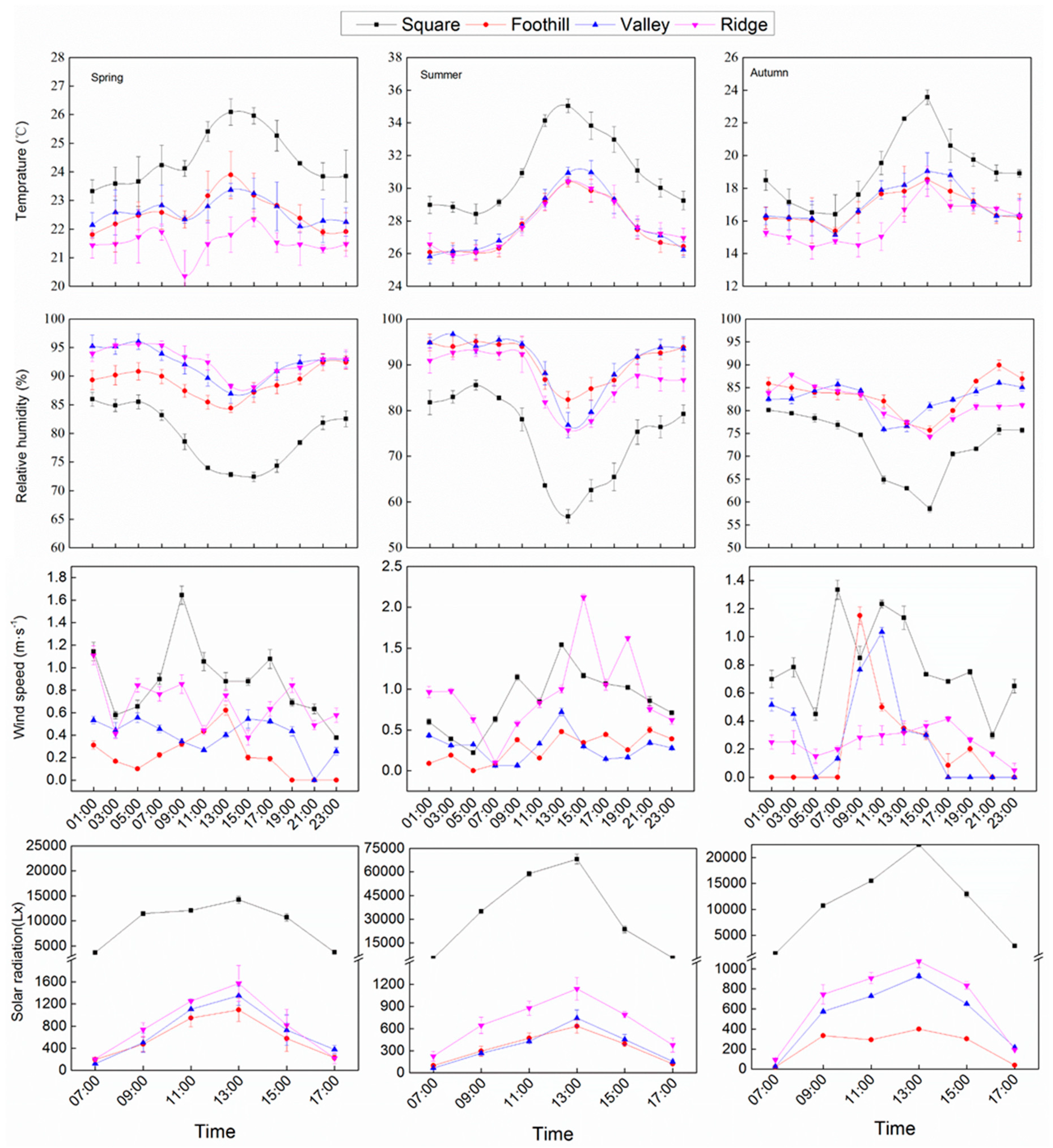
3.2. Micrometeorological Parameters

Figure 5 shows that the average diurnal cycles of AT, RH, and SR, but not of WS, in the three seasonal monitoring periods were similar for the four monitoring sites. In particular, hourly AT values steadily increased from 01:00 to reach a maximum between 13:00 and 17:00 and then decreased during the evening hours. Additionally, the daily variation curves for the three forest sites were milder than those for the square and spring curves were flatter than those observed in the other two seasons for the four sites.
For RH, the diurnal cycles for all sites were opposite to those of AT in each season. Specifically, the hourly values steadily declined from 01:00, reaching a minimum between 13:00 and 15:00 and then gradually increasing. In addition, the RH values of the three forest sites were all significantly higher than that of the square in each season.
With regard to WS, the daily variation at the four sites was unstable in each season, with large WS values typically observed in the daytime (07:00–17:00) and low values in the night-time hours (19:00–05:00). Furthermore, the hourly WS values at the four sites were all lower than 2 m s−1.
In each season, the SR values for the four sites exhibited a gradual rise from 07:00, reaching a maximum at 13:00 and then decreasing. The hourly SR values for the three forest sites were all significantly lower than that for the square.

3.3. Correlation of O3 Concentration with Micrometeorological Parameters

Table 2 presents the results of Pearson correlation analysis, which reveal that the correlation between O3 concentration and micrometeorological factors is site- and season-dependent. In spring, for all sites, O3 concentration was significantly negatively correlated with AT (r = −0.838, p < 0.0001 for foothill forestation; r = −0.693, p < 0.0005 for valley forestation; r = −0.655, p < 0.0005 for ridge forestation; r = −0.534, p = 0.001 for the square) and RH (r = −0.656, p < 0.0005 for foothill forestation; r = −0.646, p < 0.0005 for valley forestation; r = −0.480, p = 0.002 for ridge forestation; r = −0.439, p = 0.007 for the square).
In summer, for all sites, O3 concentration was significantly positively correlated with AT (r = 0.485, p = 0.003 for foothill forestation; r = 0.780, p < 0.0005 for valley forestation; r = 0.657, p < 0.0005 for ridge forestation; r = 0.825, p < 0.0001 for the square) and significantly negatively correlated with RH (r = −0.382, p = 0.022 for foothill forestation; r = −0.677, p < 0.0005 for valley forestation; r = −0.590, p < 0.0005 for ridge forestation; r = −0.806, p < 0.0001 for the square).
In autumn, O3 concentration was significantly positively correlated with AT (r = 0.634, p < 0.0005 for foothill forestation; r = 0.583, p < 0.0005 for valley forestation; r = 0.499, p = 0.002 for ridge forestation; r = 0.756, p < 0.0005 for the square) and significantly negatively correlated with RH for foothill forestation, valley forestation, and the square (r = −0.389, p = 0.019; r = −0.441, p = 0.007; r = −0.587, p < 0.0005, respectively). However, O3 concentration was generally not significantly correlated with WS or SR in any season.

4. Discussion

4.1. Effect of Urban Forests on O3 Levels

The impact of urban forests or tree canopies on O3 concentration has been investigated by performing measurements inside and outside forests using passive samplers, but the results obtained have not been consistent. In this study, the simultaneous monitoring of O3 levels in three kinds of urban forest representing different habitats and in a square with few trees showed that the effects of urban forests on O3 vary with their habitat type. The spring and autumn [O3]MDA8 values of foothill and valley forestation decreased significantly by over 15% compared to those of the square; this indicates that these urban forest types can reduce O3 levels in those two seasons. Some scholars have reported based on direct empirical measurements that urban forests have the effect of reducing O3 levels. For example, Yli-Pelkonen et al. [35] and Harris and Manning [36] showed that O3 levels in tree-covered areas were significantly lower than those in adjacent open areas. Fantozzi et al. [37] reported that O3 concentrations under Quercus ilex canopies were lower than those in open-field areas, but only in autumn. The results of this study are generally consistent with the findings of those studies. However, in this study the overall levels of O3 in ridge forestation were significantly higher than the values measured in the square; these results suggest that the level of O3 in ridge-type urban forest exhibits accumulation effects. This is much more likely ascribed to that the ridge site is intercepting airmasses that have been less influenced by near-surface deposition and titration by NOx. In addition, according to the forest canopy cover data shown on the Table 1, the value of ridge forest was lower than that of foothill and valley forest, leading to more solar radiation entering into it, and causing greater photochemical formation of O3. On the other hand, the transport of BVOCs from foothill and/or valley to ridge by mountain valley breezes during daytime could induce their accumulation as O3 precursors and thus promote the photochemical formation of O3. In our study, the summer O3 levels in the three urban forests were significantly higher than the values in the square, indicating that O3 in urban forests accumulates in summer. These results are in agreement with the findings of Yli-Pelkonen et al. [38] and Grundstrom and Pleijel [39]. This behaviour can be ascribed to (a) the emission of BVOCs (primarily isoprene or monoterpenes) from dominant species such as Acacia mangium, Schima superba, and Schefflera heptaphylla in the three forests [40,41], which enhance the photochemical production of O3 and (b) the fact that the levels of (mainly traffic-emitted) NOx in the square exceeded those in the forests, which could lead to increased O3 loss in the former case [42]. Notably, both of the above effects were most pronounced in summer. Sea–land breezes may be another important factor accounting for the differences between the forests and the square, i.e., land breezes during daytime could bring O3 from the square into forests and thus induce O3 accumulation [43].
In addition, the spring and autumn [O3]DA values for the square were significantly lower than the background data, which suggests that these urban forests do not increase local O3 levels during those seasons. The summer [O3]DA for the square, on the other hand, was significantly higher than the background data, indicating that these urban forests may increase local O3 levels in summer. However, the O3 levels in the three kinds of urban forest did not exceed the NAAQS Grade I threshold, thus demonstrating that the overall air quality of these urban forests is good and suitable for recreation purposes. Additionally, the effect of urban mountain forestation on O3 may differ from that of other types of urban forest, such as road shelter forest and residential green space. In this study, we chose only three types of urban forest representing different habitats to investigate the effect of urban forest on O3. In order to further clarify the role of urban forests in O3, we suggest that more systematic studies on O3 levels in urban forests representing a wider variety of habitats be conducted.

4.2. Dynamic Change in O3 Levels in Urban Forests

4.2.1. Spatial Variation of O3 Levels

In our results, the levels of O3 in ridge forestation (elevation 332 m) in each season were significantly higher than those for valley forestation (elevation 174 m) and foothill forestation (elevation 158 m), although the difference in O3 levels between valley and foothill elevations was not obvious (Figure 2 and Figure 3). From foothill elevation to ridge elevation, O3 levels in the urban forests tended to increase. This result is consistent with those of previous studies conducted in mountain areas [44,45,46], most of which demonstrated that the concentration of O3 increases with altitude. For example, Guo et al. [47] conducted simultaneous field measurements at various elevations on Tai Mo Shan (a mountain located in Hong Kong) and found that the O3 concentration was greater near the summit than at the foot of the mountain and similar results were obtained in a study carried out in the Southern Rocky Mountains [48]. Moreover, an investigation of O3 content in Aspe (France) and Canfranc (Spain) valleys showed that the mean O3 concentration increases upon moving from the valley bottom to the upper parts [49]. Reasons for this tendency may be explained by the fact that from foothill to ridge, the forest canopy closure gradually decreases, allowing more solar radiation to enter the forest, leading to greater photochemical formation of O3. On the other hand, the transport of BVOCs (including isoprene, mono-/sesquiterpenes, and oxygenated compounds) as O3 precursors from foothill and/or valley to ridge by mountain valley breezes during daytime could induce the accumulation of these species and thus promote the photochemical formation of O3 [50,51,52]. In addition, the increases in WS and SR from foothill to ridge (related to forest structure and topography differences; Figure 5) could also result in O3 level discrepancies between sites. The relationship between WS and SR and O3 concentration in urban forests is discussed in detail in Section 4.3.
Compared to mountainous areas, urban forests are more frequently affected by urban artificial environments—e.g., urban heat islands, traffic emissions, and human disturbance—which can promote BVOC emissions [53] and the spatial variation of O3 concentration in urban forests may differ from that in mountainous areas. In this study, however, the spatial distribution of O3 in urban forests representing three types of habitat is similar to that in mountain areas; this may be attributable to the better background air environment in the city of Shenzhen. For cities where air pollution is more serious, further study is needed to determine whether the spatial distribution of O3 in urban forest presents the same characteristics.

4.2.2. Seasonal Variation of O3 Levels

Of the seasons, the highest O3 concentrations in the sites with three kinds of urban forest in Yuanshan Forest Park were observed in summer (Figure 3), in agreement with the results of most previous studies conducted in urban, rural, and forest areas [54,55,56,57,58], and in compliance with the seasonal variation of O3 levels in Joshua Tree National Park, (Californiam, USA) [59], as well as with the seasonal variation under tree canopies in the urban area of Siena, Italy [37]. This finding can be attributed primarily to the high BVOC levels observed in this period, especially during daytime, when tree activity and the intensity of photochemical reactions are at a maximum [60,61]. However, Wang et al. [62] characterizing the levels of surface O3 in Hong Kong, found that at most sites, maximum and minimum concentrations were observed in autumn and in summer, respectively. The difference between our study’s finding and that of Wang et al. [62] may be due to differences in the seasonal cycles of sea-land breezes and wind direction.
The levels of O3 in foothill forestation were significantly higher in spring than in autumn, whereas the reverse was true for ridge forestation; levels in the valley did not show a marked seasonal variation, which can be ascribed to the fact that the seasonal variation of BVOC emissions depends on the tree species, canopy cover, and/or forest microtopography [63,64]. The high levels of O3 in foothill forestation can be explained by the increased BVOC emissions in spring [65], whereas the microtopography of the valley is thought to facilitate the formation of an inversion layer in spring and autumn, which is not conducive to the diffusion of O3. On the other hand, one of the main valley species, Ficus virens, has been reported to be a poor isoprene emitter, resulting in the stable photochemical formation of O3 in spring and autumn. For ridge forestation, the high levels of O3 in autumn can be ascribed mainly to the high elevation of this area, which favours the formation of a stable boundary layer during this season and thus facilitates the NO-promoted decomposition of O3. Thus, both our results and those previously obtained confirm the important influence of BVOCs (mainly isoprene and terpenes) on the seasonal variation of O3 levels in urban forests, highlighting the need for future synchronous studies of O3 and BVOC levels in such forests to clarify the corresponding quantisation relationship and thereby facilitate the construction of better recreational forest areas.
With regard to the daily variation of O3 concentration, the diurnal cycles of all three urban forests feature a typical shape during the spring and summer periods similar to those observed in many previous studies [43,58,59,66,67]. Specifically, relatively stable concentrations were observed from midnight to early morning (with a minimum observed in the night-time or morning hours), then a maximum between 13:00 and 15:00, followed by a decrease until midnight. This trend can be explained by the diurnal cycling of O3 source and sink levels. During the night, when photochemical production of O3 does not occur, the titration of O3 by NO becomes the dominant chemical process, leading to significant O3 loss. At night, the main sources of NO in forests are from outside the area (transported in) and from soil microbial activities [68]. The night-time loss of O3, on the other hand, can be caused by its stomatal absorption by trees and by non-stomatal removal through deposition to ground surfaces and leaf cuticles [18,69]. However, the role of these pathways is limited, which in combination with the decreased height of the night-time boundary layer, leads to fast loss of O3. Thus, the O3 concentration is minimal just before sunrise because of the overnight depletion. After sunrise, the O3 concentration begins to increase as a result of photochemical reactions and BVOC emission triggered by solar radiation. The progressively increasing difference between temperatures inside and outside the forest results in a strengthening of air convection, thus facilitating the transport of O3 and its outside precursors into the forest, causing a constant superposition and accumulation of O3. At noon, there is the most photochemical production of O3 with the largest solar radiation and enhances the accumulation of O3 so that it reaches a maximum level in the afternoon. Subsequently, the progressive decrease in solar radiation intensity results in decreased emission of BVOCs, thus promoting O3 depletion.
The diurnal curves of O3 concentration obtained for autumn feature an additional small peak at nightfall or dawn. This observation can be explained by the ease of inversion layer formation in the night-time during this season, which is conducive to the intrusion of O3-rich air from aloft down to the forest and results in O3 accumulation, in agreement with the results of a study conducted in the Pearl River Delta [18,69,70]. In addition, we found that the times at which O3 levels reached maxima or minima were slightly different between urban forests in each season, which might be related to differences in the factors affecting O3 sources and sinks, e.g., forest tree composition and/or the daily variation of micrometeorological parameter values between sites.

4.3. Impact of Micrometeorological Parameters on O3 Levels

Urban forest forms a microclimate that differs from that of an urban environment because of its ecological characteristics such as its large canopy cover, the special underlying surface, and the physiological activities of plants [71,72,73]. Microclimate parameters such as air temperature, relative humidity, wind speed, and solar radiation may play an important role in the formation, dispersion, and transport of O3 [74,75,76].
In this study, we examined the relationship between O3 concentrations and micrometeorological variables in urban forests to understand the effects of microclimate on O3 levels. The results demonstrate that O3 concentration is significantly positively correlated with AT in summer and autumn; this is similar to the finding of many existing studies in the literature [56,58,77]. However, we also found that the correlation between O3 and AT varies with the season and that AT is significantly negatively correlated with O3 in spring. This behavior can be explained mainly by the fact that temperature influences O3 levels in forests by influencing many temperature-dependent reactions, such as photochemical reactions of O3 formation and chemical titration of O3 loss [57]. In summer, although the solar radiation is strongest outside the forest, trees grow vigorously and the forest canopy cover is larger, which has the greatest reduction on solar radiation, so the light entering the forest is less than that in spring. However, during this season, trees have the largest emission of BVOCs and temperature affects O3 levels in the forest mainly by influencing the rate of photochemical O3 formation (i.e., elevated temperatures promote BVOC emission) and thus accelerate the rate of photochemical O3 generation, so that O3 concentration is significantly positively correlated with AT. In addition, based on the findings of this study, solar radiation which is related to photochemical reaction to form O3 in forest locations is significantly higher in the spring than in the summer. Spring is characterized by the onset of the physiological activity of trees, at which time the new leaves of trees are in the stage of germination and the canopy cover of forests is relatively low. At the same time, the solar radiation increases with the increase of the solar altitude angle, while the reduction of tree canopy on solar radiation, such as reflection and scattering, is less. Therefore, the solar radiation flux into the forest is more and the solar radiation is stronger, which may cause more photochemical formation of O3 at higher temperature. However, an anti-correlation between O3 and air temperature is seen at all of the sites in spring and this may be due to the effect of air temperature on the boundary layer height. A high boundary layer height means a better dispersion condition, which may spread O3 to aloft and decrease O3 in the surface. The decrease of air temperature may cause the dropping of boundary layer, which is not conducive to the dispersion of O3, and can cause the accumulation of O3. In addition, the decrease of boundary layer may also be conducive to the sinking of O3-rich air from aloft into the forest to increase O3 concentrations. However, based on the findings of this study and previous studies, it is still unclear why this correlation is seen. Therefore, we suggest that further in-depth studies on the relationship between temperature and O3 in different seasons should be carried out in order to clarify the effect of temperature on O3 levels in urban forest.
With regard to the relationship between O3 concentrations and RH, a negative correlation was found for each season; this is consistent with most previous studies [58,76,78]. The reasons may be explained as follows. On the one hand, O3 can deposit on water droplets. On the other hand, O3 photolysis, followed by reaction of the O(1D) atom produced with water would increase at higher RH, and therefore contributes to O3 loss. The formation of large amounts of water vapour at high RH increases the degree of solar radiation scattering and therefore negatively affects the photochemical production of O3.
Many studies in urban areas have pointed out that O3 is positively correlated with WS because of the dependence of the diffusion and transport of O3 on WS. However, the results of Sari et al. [58], in a study of the relationship between surface O3 levels and WS in the forest area of the Biga Peninsula, Turke, show that the correlation coefficient between surface O3 and WS is not high. In our study, the O3 concentration was not found to be significantly correlated with WS and this agrees with the findings of Sari et al. [58]. This behavior can be ascribed to the fact that during our monitoring period, WS values in the forests usually did not exceed 2 m s−1, whereas the tendency of forest air to form turbulent flows caused the wind speed and direction to be unstable during daytime. Therefore, under these conditions, WS had little effect on the diffusion and transport of O3. In addition, we found that solar radiation did not significantly affect the concentration of O3 in the forests, in contrast to results previously reported by Shan et al. [76], Zhao et al. [78], and other researchers. This difference may be related to the fact that forest crowns can significantly reduce solar radiation. In addition, a large number of investigations have shown that forest microclimate parameters such as AT, RH, WS, and SR are strongly affected by or dependent on certain ecological characteristics of forests such as tree density, speciation, canopy density, and leaf area index [79,80,81]. Based on this, we suggest that micrometeorological parameter values can be adjusted by changing the above factors to control O3 levels in urban forests.

5. Conclusions

In this study, we used portable monitors to synchronously record O3 concentrations and meteorological parameters in three types of forest representing common habitats of Yuanshan Forest Park and an adjacent square from August 2015 to April 2016. The results include the following observations and findings:
The effects of urban forests on O3 vary with their habitat type: In ridge urban forestation, O3 accumulates in all seasons, but in foothill and valley urban forests, it decreases in spring and autumn.
From foothill elevations to ridge elevations, the O3 concentrations in the forests gradually increased, indicating that the air quality of urban forests in foothill and valley forests is better than that of ridge forestation.
For all forest sites, the highest O3 concentrations were observed in summer; this seems to be related to the fact that BVOC emissions during this period are at a maximum. Thus, air quality of the urban forests in spring and autumn was better than that in summer. The levels of O3 were always high in the afternoon (13:00–17:00) and lower at night or in the early morning (03:00–09:00); this means that the best times for residents to participate in recreational activities in the forests are before 09:00.
In the urban forests, O3 concentration was significantly correlated with AT and RH but not with WS and SR; i.e., AT and/or RH may be the main micrometeorological factors influencing the O3 levels. This suggests that when the habitat of urban forest is known, we can regulate the forest characteristics that affect the microclimate, such as tree density, to reduce O3 levels in the forests.
MDA8 and hourly concentrations of O3 in the three types of urban forest in Yuanshan Forest Park did not exceed the NAAQS Grade I thresholds of 100 and 160 μg m−3, respectively, during the entire monitoring period. Thus, the air quality of these urban forests is good and is suitable for recreation purposes.

Author Contributions

W.D. analyzed data and drafted the manuscript. C.W. was involved in planning of study and designing of the work. N.P., C.Z., Z.H., and X.X. participated in collecting the experiment data. The remaining authors (L.G. and S.J.) contributed to refining the ideas, carrying out additional analyses and finalizing this paper. All authors discussed the results and revised the manuscript.

Funding

This work was supported by Special Fund for Forestry Scientific Research in the Public Interest (No. 201404301), the National Science and Technology Pillar Program during the 13th Five-year Plan Period (No. 2015BAD07B06) and the National Natural Science Foundation of China (31570594).

Acknowledgments

We are grateful to the Editor and the three anonymous reviewers for their valuable advices and conscientious work.

Conflicts of Interest

The authors declare no conflict of interest.

References

  1. Liu, H.; Li, F.; Li, J.; Zhang, Y. The relationships between urban parks, residents’ physical activity, and mental health benefits: A case study from Beijing, China. J. Environ. Manag. 2017, 190, 223–230. [Google Scholar] [CrossRef] [PubMed]
  2. Tsunetsugu, Y.; Lee, J.; Park, B.J.; Tyrväinen, L.; Kagawa, T.; Miyazaki, Y. Physiological and psychological effects of viewing urban forest landscapes assessed by multiple measurements. Landsc. Urban Plan. 2013, 113, 90–93. [Google Scholar] [CrossRef]
  3. Arnberger, A.; Eder, R. Exploring coping behaviours of Sunday and workday visitors due to dense use conditions in an urban forest. Urban For. Urban Green. 2012, 11, 439–449. [Google Scholar] [CrossRef]
  4. Chen, B.; Qi, X. Protest response and contingent valuation of an urban forest park in Fuzhou City, China. Urban For. Urban Green. 2018, 29, 68–76. [Google Scholar] [CrossRef]
  5. Wolf, I.D.; Wohlfart, T. Walking, hiking and running in parks: A multidisciplinary assessment of health and well-being benefits. Landsc. Urban Plan. 2014, 130, 89–103. [Google Scholar] [CrossRef]
  6. Chan, L.Y.; Chan, C.Y.; Qin, Y. Surface Ozone Pattern in Hong Kong. J. Appl. Meteorol. 1998, 37, 1153–1165. [Google Scholar] [CrossRef]
  7. Calfapietra, C.; Fares, S.; Manes, F.; Morani, A.; Sgrigna, G.; Loreto, F. Role of Biogenic Volatile Organic Compounds (BVOC) emitted by urban trees on ozone concentration in cities: A review. Environ. Pollut. 2013, 183, 71–80. [Google Scholar] [CrossRef] [PubMed]
  8. Francesco, L.; Schnitzler, J.-P. Abiotic stresses and induced BVOCs. Trends Plant Sci. 2010, 15, 154–166. [Google Scholar]
  9. Malmqvist, E.; Olsson, D.; Hagenbjörk-Gustafsson, A.; Forsberg, B.; Mattisson, K.; Stroh, E.; Strömgren, M.; Swietlicki, E.; Rylander, L.; Hoek, G. Assessing ozone exposure for epidemiological studies in Malmö and Umeå, Sweden. Atmos. Environ. 2014, 94, 241–248. [Google Scholar] [CrossRef] [Green Version]
  10. Tao, Y.; Huang, W.; Huang, X.; Zhong, L.; Lu, S.E.; Li, Y.; Dai, L.; Zhang, Y.; Zhu, T. Estimated acute effects of ambient ozone and nitrogen dioxide on mortality in the pearl river delta of southern China. Environ. Health Perspect. 2012, 120, 393. [Google Scholar] [CrossRef] [PubMed]
  11. Uysal, N.; Schapira, R.M. Effects of ozone on lung function and lung diseases. Curr. Opin. Pulm. Med. 2003, 9, 144–150. [Google Scholar] [CrossRef] [PubMed]
  12. Bates, D.V. Ambient ozone and mortality. Epidemiology 2005, 16, 427–429. [Google Scholar] [CrossRef] [PubMed]
  13. Liu, H.; Liu, S.; Xue, B.; Lv, Z.; Meng, Z.; Yang, X.; Xue, T.; Yu, Q.; He, K. Ground-level ozone pollution and its health impacts in China. Atmos. Environ. 2018, 173, 223–230. [Google Scholar] [CrossRef]
  14. Nowak, D.J.; Hirabayashi, S.; Doyle, M.; Mcgovern, M.; Pasher, J. Air pollution removal by urban forests in canada and its effect on air quality and human health. Urban For. Urban Green. 2018, 29, 40–48. [Google Scholar] [CrossRef]
  15. Manes, F.; Marando, F.; Capotorti, G.; Blasi, C.; Salvatori, E.; Fusaro, L.; Ciancarella, L.; Mircea, M.; Marchetti, M.; Chirici, G.; et al. Regulating ecosystem services of forests in ten Italian metropolitan cities: Air quality improvement by PM10 and O3 removal. Ecol. Indic. 2016, 67, 425–440. [Google Scholar] [CrossRef]
  16. Bottalico, F.; Chirici, G.; Giannetti, F.; De Marco, A.; Nocentini, S.; Paoletti, E.; Salbitano, F.; Sanesi, G.; Serenelli, C.; Travaglini, D. Air pollution removal by green infrastructures and urban forests in the city of Florence. Agric. Agric. Sci. Procedia 2016, 8, 243–251. [Google Scholar] [CrossRef]
  17. Selmi, W.; Weber, C.; Rivière, E.; Blond, N.; Mehdi, L.; Nowak, D. Air pollution removal by trees in public green spaces in Strasbourg city, France. Urban For. Urban Green. 2016, 17, 192–201. [Google Scholar] [CrossRef] [Green Version]
  18. Cape, J.N.; Hamilton, R.; Heal, M.R. Reactive uptake of ozone at simulated leaf surfaces: Implications for ‘non-stomatal’ ozone flux. Atmos. Environ. 2009, 43, 1116–1123. [Google Scholar] [CrossRef] [Green Version]
  19. Kitao, M.; Komatsu, M.; Hoshika, Y.; Yazaki, K.; Yoshimura, K.; Fujii, S.; Miyama, T.; Kominami, Y. Seasonal ozone uptake by a warm-temperate mixed deciduous and evergreen broadleaf forest in western Japan estimated by the Penman-Monteith approach combined with a photosynthesis-dependent stomatal model. Environ. Pollut. 2014, 184, 457–463. [Google Scholar] [CrossRef] [PubMed]
  20. Wang, H.; Zhou, W.; Wang, X.; Gao, F.; Zheng, H.; Tong, L.; Ouyang, Z. Ozone uptake by adult urban trees based on sap flow measurement. Environ. Pollut. 2012, 162, 275–286. [Google Scholar] [CrossRef] [PubMed] [Green Version]
  21. Chatani, S.; Matsunaga, S.N.; Nakatsuka, S. Estimate of biogenic VOC emissions in Japan and their effects on photochemical formation of ambient ozone and secondary organic aerosol. Atmos. Environ. 2015, 120, 38–50. [Google Scholar] [CrossRef]
  22. Paoletti, E. Ozone and urban forests in Italy. Environ. Pollut. 2009, 157, 1506–1512. [Google Scholar] [CrossRef] [PubMed]
  23. Feng, Z.; Li, P. Effects of Ozone on Chinese Trees. Air Pollution Impacts on Plants in East Asia; Springer: Tokyo, Japan, 2017; pp. 195–219. [Google Scholar]
  24. Gao, F.; Calatayud, V.; García-Breijo, F.; Reig-Armiñana, J.; Feng, Z. Effects of elevated ozone on physiological, anatomical and ultrastructural characteristics of four common urban tree species in China. Ecol. Indic. 2016, 67, 367–379. [Google Scholar] [CrossRef] [Green Version]
  25. Zhang, W.; Feng, Z.; Wang, X.; Niu, J. Elevated ozone negatively affects photosynthesis of current-year leaves but not previous-year leaves in evergreen Cyclobalanopsis glauca seedlings. Environ. Pollut. 2014, 184, 676–681. [Google Scholar] [CrossRef] [PubMed] [Green Version]
  26. Ling, Z.H.; Guo, H.; Cheng, H.R.; Yu, Y.F. Sources of ambient volatile organic compounds and their contributions to photochemical ozone formation at a site in the Pearl River Delta, southern China. Environ. Pollut. 2011, 159, 2310–2319. [Google Scholar] [CrossRef] [PubMed]
  27. Mo, Z.; Shao, M.; Wang, W.; Liu, Y.; Wang, M.; Lu, S. Evaluation of biogenic isoprene emissions and their contribution to ozone formation by ground-based measurements in Beijing, China. Sci. Total Environ. 2018, 627, 1485–1494. [Google Scholar] [CrossRef]
  28. Han, X.; Huang, X.; Liang, H.; Ma, S.; Gong, J. Analysis of the relationships between environmental noise and urban morphology. Environ. Pollut. 2018, 233, 755–763. [Google Scholar] [CrossRef] [PubMed]
  29. Aeroqual. Aeroqual Series 200/300/500 User Guide. Available online: http://www.aeroqual.com (accessed on 25 October 2014).
  30. Aeroqual. Portable and Fixed Monitor Gas Sensor Specifications. Available online: http://www.aeroqual com (accessed on 11 November 2014).
  31. Lin, C.; Gillespie, J.; Schuder, M.D.; Duberstein, W.; Beverland, I.J.; Heal, M.R. Evaluation and calibration of Aeroqual series 500 portable gas sensors for accurate measurement of ambient ozone and nitrogen dioxide. Atmos. Environ. 2015, 100, 111–116. [Google Scholar] [CrossRef] [Green Version]
  32. McKercher, G.R.; Salmond, J.A.; Vanos, J.K. Characteristics and applications of small, portable gaseous air pollution monitors. Environ. Pollut. 2017, 223, 102–110. [Google Scholar] [CrossRef] [PubMed] [Green Version]
  33. Minet, L.; Gehr, R.; Hatzopoulou, M. Capturing the sensitivity of land-use regression models to short-term mobile monitoring campaigns using air pollution micro-sensors. Environ. Pollut. 2017, 230, 280–290. [Google Scholar] [CrossRef] [PubMed]
  34. Wang, D.P.; Ji, S.Y.; Chen, F.P.; Xing, F.W.; Peng, S.L. Diversity and relationship with succession of naturally regenerated southern subtropical forests in Shenzhen, China and its comparison with the zonal climax of Hong Kong. For. Ecol. Manag. 2006, 222, 384–390. [Google Scholar] [CrossRef]
  35. Yli-Pelkonen, V.; Scott, A.A.; Viippola, V.; Setälä, H. Trees in urban parks and forests reduce O3, but not NO2 concentrations in Baltimore, MD, USA. Atmos. Environ. 2017, 167, 73–80. [Google Scholar] [CrossRef]
  36. Harris, T.B.; Manning, W.J. Nitrogen dioxide and ozone levels in urban tree canopies. Environ. Pollut. 2010, 158, 2384–2386. [Google Scholar] [CrossRef] [PubMed]
  37. Fantozzi, F.; Monaci, F.; Blanusa, T.; Bargagli, R. Spatio-temporal variations of ozone and nitrogen dioxide concentrations under urban trees and in a nearby open area. Urban Clim. 2015, 12, 119–127. [Google Scholar] [CrossRef]
  38. Yli-Pelkonen, V.; Setälä, H.; Viippola, V. Urban forests near roads do not reduce gaseous air pollutant concentrations but have an impact on particles levels. Landsc. Urban Plan. 2017, 158, 39–47. [Google Scholar] [CrossRef]
  39. Grundstrom, M.; Pleijel, H. Limited effect of urban tree vegetation on NO2 and O3 concentrations near a traffic route. Environ. Pollut. 2014, 189, 73–76. [Google Scholar] [CrossRef] [PubMed]
  40. Singh, R.; Singh, M.P.; Singh, A.P. Ozone forming potential of tropical plant species of the Vidarbha region of Maharashtra state of India. Urban For. Urban Green. 2014, 13, 814–820. [Google Scholar] [CrossRef]
  41. Tsui, J.K.-Y.; Guenther, A.; Yip, W.-K.; Chen, F. A biogenic volatile organic compound emission inventory for Hong Kong. Atmos. Environ. 2009, 43, 6442–6448. [Google Scholar] [CrossRef] [Green Version]
  42. Sillman, S. The relation between ozone, NOx and hydrocarbons in urban and polluted rural environments. Elsevier Sci. Technol. 1999, 33, 1821–1845. [Google Scholar] [CrossRef]
  43. Shan, W.; Zhang, J.; Huang, Z.; You, L. Characterizations of ozone and related compounds under the influence of maritime and continental winds at a coastal site in the Yangtze Delta, nearby Shanghai. Atmos. Res. 2010, 97, 26–34. [Google Scholar] [CrossRef]
  44. Gao, J.; Wang, T.; Ding, A.; Liu, C. Observational study of ozone and carbon monoxide at the summit of mount Tai (1534 m a.s.l.) in central-eastern China. Atmos. Environ. 2005, 39, 4779–4791. [Google Scholar] [CrossRef]
  45. Sun, Y.; Wang, L.; Wang, Y.; Zhang, D.; Quan, L.; Jinyuan, X. In situ measurements of NO, NO2, NOy, and O3 in Dinghushan (112° E, 23° N), China during autumn 2008. Atmos. Environ. 2010, 44, 2079–2088. [Google Scholar] [CrossRef]
  46. Xue, L.K.; Wang, T.; Zhang, J.M.; Zhang, X.C.; Poon, C.N.; Ding, A.J.; Zhou, X.H.; Wu, W.S.; Tang, J.; Zhang, Q.Z.; et al. Source of surface ozone and reactive nitrogen speciation at Mount Waliguan in western China: New insights from the 2006 summer study. J. Geophys. Res. 2011, 116. [Google Scholar] [CrossRef] [Green Version]
  47. Guo, H.; Ling, Z.H.; Cheung, K.; Jiang, F.; Wang, D.W.; Simpson, I.J.; Barletta, B.; Meinardi, S.; Wang, T.J.; Wang, X.M.; et al. Characterization of photochemical pollution at different elevations in mountainous areas in Hong Kong. Atmos. Chem. Phys. 2013, 13, 3881–3898. [Google Scholar] [CrossRef] [Green Version]
  48. Musselman, R.C.; Korfmacher, J.L. Ozone in remote areas of the Southern Rocky Mountains. Atmos. Environ. 2014, 82, 383–390. [Google Scholar] [CrossRef]
  49. Ezcurra, A.; Benech, B.; Echelecou, A.; Santamaría, J.M.; Herrero, I.; Zulueta, E. Influence of local air flow regimes on the ozone content of two Pyrenean valleys. Atmos. Environ. 2013, 74, 367–377. [Google Scholar] [CrossRef]
  50. Kim, S.-Y.; Jiang, X.; Lee, M.; Turnipseed, A.; Guenther, A.; Kim, J.-C.; Lee, S.-J.; Kim, S. Impact of biogenic volatile organic compounds on ozone production at the Taehwa Research Forest near Seoul, South Korea. Atmos. Environ. 2013, 70, 447–453. [Google Scholar] [CrossRef] [Green Version]
  51. Lee, B.; Wang, J. Concentration variation of isoprene and its implications for peak ozone concentration. Atmos. Environ. 2006, 40, 5486–5495. [Google Scholar] [CrossRef]
  52. Pang, X.; Mu, Y.; Zhang, Y.; Lee, X.; Yuan, J. Contribution of isoprene to formaldehyde and ozone formation based on its oxidation products measurement in Beijing, China. Atmos. Environ. 2009, 43, 2142–2147. [Google Scholar] [CrossRef] [Green Version]
  53. Ghirardo, A.; Xie, J.; Zheng, X.; Wang, Y.; Grote, R.; Block, K.; Wildt, J.; Mentel, T.; Kiendler-Scharr, A.; Hallquist, M.; et al. Urban stress-induced biogenic VOC emissions and SOA-forming potentials in Beijing. Atmos. Chem. Phys. 2016, 16, 2901–2920. [Google Scholar] [CrossRef] [Green Version]
  54. Adame, J.A.; Sole, J.G. Surface ozone variations at a rural area in the northeast of the Iberian Peninsula. Atmos. Pollut. Res. 2013, 4, 130–141. [Google Scholar] [CrossRef] [Green Version]
  55. Fernandez-Guisuraga, J.M.; Castro, A.; Alves, C.; Calvo, A.; Alonso-Blanco, E.; Blanco-Alegre, C.; Rocha, A.; Fraile, R. Nitrogen oxides and ozone in Portugal: Trends and ozone estimation in an urban and a rural site. Environ. Sci. Pollut. Res. Int. 2016, 23, 17171–17182. [Google Scholar] [CrossRef] [PubMed]
  56. Martin, P.; Cabañas, B.; Villanueva, F.; Gallego, M.P.; Colmenar, I.; Salgado, S. Ozone and nitrogen dioxide levels monitored in an urban area (Ciudad Real) in central-southern Spain. Water Air Soil Pollut. 2009, 208, 305–316. [Google Scholar] [CrossRef]
  57. Notario, A.; Diaz-de-Mera, Y.; Aranda, A.; Adame, J.A.; Parra, A.; Romero, E.; Parra, J.; Munoz, F. Surface ozone comparison conducted in two rural areas in central-southern Spain. Environ. Sci. Pollut. Res. Int. 2012, 19, 186–200. [Google Scholar] [CrossRef] [PubMed]
  58. Sari, D.; Incecik, S.; Ozkurt, N. Surface ozone levels in the forest and vegetation areas of the Biga Peninsula, Turkey. Sci. Total Environ. 2016, 571, 1284–1297. [Google Scholar] [CrossRef] [PubMed]
  59. Burley, J.D.; Bytnerowicz, A.; Ray, J.D.; Schilling, S.; Allen, E.B. Surface ozone in Joshua Tree National Park. Atmos. Environ. 2014, 87, 95–107. [Google Scholar] [CrossRef]
  60. Li, L.Y.; Chen, Y.; Xie, S.D. Spatio-temporal variation of biogenic volatile organic compounds emissions in China. Environ. Pollut. 2013, 182, 157–168. [Google Scholar] [CrossRef] [PubMed]
  61. Son, Y.S.; Kim, K.J.; Jung, I.H.; Lee, S.J.; Kim, J.C. Seasonal variations and emission fluxes of monoterpene emitted from coniferous trees in East Asia: Focused on Pinus rigida and Pinus koraiensis. J. Atmos. Chem. 2015, 72, 27–41. [Google Scholar] [CrossRef]
  62. Wang, T.; Cheung, T.F.; Lam, K.S.; Wu, Y.Y. A study of surface ozone and the relation to complex wind flow in Hong Kong. Atmos. Environ. 2001, 35, 3203–3215. [Google Scholar] [CrossRef]
  63. Lim, Y.J.; Armendariz, A.; Son, Y.-S.; Kim, J.C. Seasonal variations of isoprene emissions from five oak tree species in East Asia. Atmos. Environ. 2011, 45, 2202–2210. [Google Scholar] [CrossRef]
  64. Taha, H.; Wilkinson, J.; Bornstein, R.; Xiao, Q.; McPherson, G.; Simpson, J.; Anderson, C.; Lau, S.; Lam, J.; Blain, C. An urban-forest control measure for ozone in the Sacramento, CA Federal Non-Attainment Area (SFNA). Sustain. Cit. Soc. 2016, 21, 51–65. [Google Scholar] [CrossRef]
  65. Ou Yang, C.F.; Lin, N.H.; Sheu, G.R.; Lee, C.T.; Wang, J.L. Seasonal and diurnal variations of ozone at a high-altitude mountain baseline station in East Asia. Atmos. Environ. 2012, 46, 279–288. [Google Scholar] [CrossRef]
  66. Filella, I.; Peñuelas, J. Daily, weekly and seasonal relationships among VOCs, NOx x and O3 in a semi-urban area near Barcelona. J. Atmos. Chem. 2006, 54, 189–201. [Google Scholar] [CrossRef]
  67. Zhang, J.; Wang, T.; Chameides, W.L.; Cardelino, C.; Kwo, J.; Blak, D.R.; Ding, A.; So, K.L. Ozone production and hydrocarbon reactivity in Hong Kong, Southern China. Atmos. Chem. Phys. 2006, 6, 557–573. [Google Scholar] [CrossRef]
  68. Su, H.; Pöschl, U. Soil nitrite as a source of atmospheric HONO and OH radicals. Science 2011, 333, 1616–1618. [Google Scholar] [CrossRef] [PubMed]
  69. Grulke, N.E.; Alonso, R.; Nguyen, T.; Cascio, C.; Dobrowolski, W. Stomata open at night in pole-sized and mature ponderosa pine: Implications for O3 exposure metrics. Tree Physiol. 2004, 24, 1001–1010. [Google Scholar] [CrossRef] [PubMed]
  70. Shao, M.; Zhang, Y.; Zeng, L.; Tang, X.; Zhang, J.; Zhong, L.; Wang, B. Ground-level ozone in the Pearl River Delta and the roles of VOC and NOx in its production. J. Environ. Manag. 2009, 90, 512–518. [Google Scholar] [CrossRef] [PubMed]
  71. Hamada, S.; Ohta, T. Seasonal variations in the cooling effect of urban green areas on surrounding urban areas. Urban For. Urban Green. 2010, 9, 15–24. [Google Scholar] [CrossRef]
  72. Tsoka, S. Investigating the relationship between urban spaces morphology and local microclimate: A study for Thessaloniki. Procedia Environ. Sci. 2017, 38, 674–681. [Google Scholar] [CrossRef]
  73. Zhang, Z.; Lv, Y.; Pan, H. Cooling and humidifying effect of plant communities in subtropical urban parks. Urban For. Urban Green. 2013, 12, 323–329. [Google Scholar] [CrossRef]
  74. Elminir, H.K. Dependence of urban air pollutants on meteorology. Sci. Total Environ. 2005, 350, 225–237. [Google Scholar] [CrossRef] [PubMed]
  75. Ooka, R.; Mai, K.; Hayami, H.; Yoshikado, H.; Huang, H.; Kawamoto, Y. Influence of meteorological conditions on summer ozone levels in the central Kanto area of Japan. Procedia Environ. Sci. 2011, 4, 138–150. [Google Scholar] [CrossRef] [Green Version]
  76. Shan, W.; Yin, Y.; Zhang, J.; Ji, X.; Deng, X. Surface ozone and meteorological condition in a single year at an urban site in central-eastern China. Environ. Monit. Assess. 2009, 151, 127–141. [Google Scholar] [CrossRef] [PubMed]
  77. Vecchi, R.; Valli, G. Ozone assessment in the southern part of the Alps. Atmos. Environ. 1999, 33, 97–109. [Google Scholar] [CrossRef]
  78. Zhao, W.; Fan, S.; Guo, H.; Gao, B.; Sun, J.; Chen, L. Assessing the impact of local meteorological variables on surface ozone in Hong Kong during 2000–2015 using quantile and multiple line regression models. Atmos. Environ. 2016, 144, 182–193. [Google Scholar] [CrossRef]
  79. Reinap, A.; Wiman, B.L.B.; Svenningsson, B.; Gunnarsson, S. Oak leaves as aerosol collectors: Relationships with wind velocity and particle size distribution. Experimental results and their implications. Trees 2009, 23, 1263–1274. [Google Scholar] [CrossRef]
  80. Wuyts, K.; Verheyen, K.; An, D.S.; Cornelis, W.M.; Gabriels, D. The impact of forest edge structure on longitudinal patterns of deposition, wind speed, and turbulence. Atmos. Environ. 2008, 42, 8651–8660. [Google Scholar] [CrossRef]
  81. Yang, J.; Mcbride, J.; Zhou, J.; Sun, Z. The urban forest in Beijing and its role in air pollution reduction. Urban For. Urban Green. 2005, 3, 65–78. [Google Scholar] [CrossRef]
Figure 1. (a) Map of China and the Guangdong province (red area), with the blue area representing the city of Shenzhen (113°46′–114°37′ E, 22°27′–22°52′ N). (b) Aerial image of Yuanshan Forest Park (red solid line), with the red circles indicating monitoring sites.
Forests 10 00247 g001
Figure 2. Mean daily and daily maximum 8 h mean (MDA8) concentrations of surface ozone (O3) ([O3]DA and [O3]MDA8, respectively) for the three types of urban forest and the square throughout the monitoring period. Bars represent the standard error of the mean for n = 6 determined for each monitoring site. Different capital letters indicate significant differences with p < 0.01, and different lower-case letters indicate significant differences with p < 0.05.
Forests 10 00247 g002
Figure 3. Seasonal and spatial variation of [O3]DA and [O3]MDA8 for the three types of urban forest and the square. Bars represent standard errors of the mean for n = 6 determined for each monitoring site. Different capital letters indicate significant differences between monitoring sites for a given season (p < 0.05), and different lower-case letters indicate significant differences between different seasons for a given monitoring site (p < 0.05).
Forests 10 00247 g003
Figure 4. Mean diurnal cycles of O3 concentration in the three types of urban forest and the square for (a) spring, (b) summer, and (c) autumn.
Forests 10 00247 g004
Figure 5. Mean diurnal cycles of air temperature (AT), relative humidity (RH), wind speed (WS), and solar radiation (SR) for the three types of urban forest and the square in spring, summer, and autumn. Note the different scales of the y-axis.
Forests 10 00247 g005
Table 1. Vegetation parameters surveyed at three forest plots. Trees with a diameter at breast height (DBH) of <0.8 cm are not included.
SiteLocationElevation/mCanopy CoverArbor Trees
Average Height/mAverage DBH/cmDominat Species
Foothill22°38′34″ N,
114°14′33″ E
1580.6510.75 ± 0.8012.97 ± 1.17Acacia mangium
Cunninghamia lanceolata
Schefflera heptaphylla
Dalbergia benthamii
Cinnamomum camphora
Valley22°38′34″ N,
114°14′33″ E
1740.757.60 ± 0.4710.48 ± 1.21Ficus virens
Schima superba
Ehretia thyrsiflora
Dalbergia benthamii
Gironniera subaequalis
Ridge22°38′34″ N,
114°14′33″ E
3320.608.58 ± 0.5113.57 ± 1.25Schima superba
Scheffleraheptaphylla
Celtis sinensis
Dalbergia benthamii
Cinnamomum camphora
Table 2. Correlations between O3 concentration and micrometeorological parameters.
SeasonSiteAir TemperatureRelative HumidityWind SpeedSolar Radiation
SpringFoothill−0.838 **−0.656 **0.497 **−0.260
Valley−0.693 **−0.646 **0.298−0.149
Ridge−0.655 **−0.480 **0.062−0.191
Square−0.534 **−0.439 *0.091−0.250
SummerFoothill0.485 **−0.382 *0.1410.256
Valley0.780 **−0.677 **0.0460.447 *
Ridge0.657 **−0.590 **0.354 *0.173
Square0.825 **−0.806 **0.493 **0.211
AutumnFoothill0.634 **−0.389 *−0.247−0.266
Valley0.583 **−0.441 **−0.0120.109
Ridge0.499 **−0.0280.171−0.207
Square0.756 **−0.587 **0.2310.573 *
* Correlation is significant at the 0.05 level (two-tailed). ** Correlation is significant at the 0.01 level (two-tailed).

