Landsat 8 Based Leaf Area Index Estimation in Loblolly Pine Plantations

Abstract

Leaf area index (LAI) is an important biophysical parameter used to monitor, model, and manage loblolly pine plantations across the southeastern United States. Landsat provides forest scientists and managers the ability to obtain accurate and timely LAI estimates. The objective of this study was to investigate the relationship between loblolly pine LAI measured in situ (at both leaf area minimum and maximum through two growing seasons at two geographically disparate study areas) and vegetation indices calculated using data from Landsat 7 (ETM+) and Landsat 8 (OLI). Sub-objectives included examination of the impact of georegistration accuracy, comparison of top-of-atmosphere and surface reflectance, development of a new empirical model for the species and region, and comparison of the new empirical model with the current operational standard. Permanent plots for the collection of ground LAI measurements were established at two locations near Appomattox, Virginia and Tuscaloosa, Alabama in 2013 and 2014, respectively. Each plot is thirty by thirty meters in size and is located at least thirty meters from a stand boundary. Plot LAI measurements were collected twice a year using the LI-COR LAI-2200 Plant Canopy Analyzer. Ground measurements were used as dependent variables in ordinary least squares regressions with ETM+ and OLI-derived vegetation indices. We conclude that accurately-located ground LAI estimates at minimum and maximum LAI in loblolly pine stands can be combined and modeled with Landsat-derived vegetation indices using surface reflectance, particularly simple ratio (SR) and normalized difference moisture index (NDMI), across sites and sensors. The best resulting model (LAI = −0.00212 + 0.3329SR) appears not to saturate through an LAI of 5 and is an improvement over the current operational standard for loblolly pine monitoring, modeling, and management in this ecologically and economically important region.

1. Introduction

Leaf area index (LAI) is widely used in silvicultural decision support [1,2]. Careful silvicultural manipulation of LAI can reduce drought stress [3], and can be used to assess site preparation outcomes, including the proportion of stand LAI post-establishment that is from competing herbaceous and arborescent species [4]. LAI has been shown to be an important predictor of site nutrient status in pine stands and can be used to determine the likelihood of forest management response [5]. Fertilization increases LAI in loblolly pine (Pinus taeda L.) stands which leads to faster growth [6,7,8]. LAI can be used by forest managers to identify stands that would likely benefit from fertilization and/or competition control [9], and, for a given species, a stand’s maximum (life cycle) LAI is strongly correlated with other measures of site quality such as site index [10].

Modern forestry thus requires satellite-derived LAI [1,2], but as noted by Gao et al. 2014 [11], the coarse scale of available satellite derived LAI estimates from the Moderate Resolution Imaging Spectroradiometer (MODIS) is not adequate for stand-scale analyses since most pine plantations in the southern U.S. contain very few or no homogeneous MODIS pixels. The promise and potential of LAI estimation in monospecific pine plantations using Landsat data was noted by Vogel et al. [12]. Thus, there is both strong potential and extant need for LAI estimates from medium resolution sensors for use in forest management.

Loblolly pine trees carry two needle cohorts at maximum LAI in late summer and one at minimum LAI in late winter resulting in an almost doubling of pine LAI between minimum and maximum [13]. Since a majority of loblolly pine plantations also have hardwood competition that contributes to LAI in seasons other than winter, empirical modeling has often focused on minimum LAI in the winter when only the pine trees have “leaves” [14]. Previous research conducted by Flores et al. [15] related top-of-atmosphere (TOA) reflectance-based simple ratio vegetation index from Landsat 7’s Enhanced Thematic Mapper Plus (ETM+) sensor to loblolly pine LAI in the winter. They indicated that others have also successfully used remote sensing to characterize the LAI of forest stands [15].

Differences between Landsat-derived estimates of LAI in spring and winter have been shown to be useful in the estimation of the relative abundance of deciduous competition in loblolly pine stands [9]. However, models for the estimation of loblolly pine LAI with satellite-based vegetation indices (VIs) have not been as successful at maximum LAI, with the exception of intensively managed slash pine with an ericaceous understory [16,17,18]. Chen and Cihlar [19] found late spring images to be better than summer images for the estimation of LAI in boreal conifer stands because of the reduced influence of the understory, a result echoed by Tian et al. [20] using the annual leaf area minimum (better model) versus maximum (worse model). For boreal forests, Chen and Cihlar [19] concluded that there is a linear relationship between SR and LAI, while Curran et al. [18] demonstrated that remote sensing could be used to study seasonal dynamics of LAI in southern slash pine plantations.

Vegetation index saturation has been a problem in forest stands with high levels of LAI [21,22,23], which is especially problematic in the summer across the southern portions of loblolly pine’s range in the U.S. Turner et al. [22] evaluated the relationship between in situ LAI estimates and Landsat Thematic Mapper (TM)-derived VIs for several cover types at three different study sites in the summer. Surface reflectance based normalized difference vegetation index (NDVI) resulted in the best model fit, but VI saturation was still noted in the coniferous stands [22]. Sumnall et al. [24] suggest that using LiDAR can reduce or remove the saturation issues in areas of high biomass.

Empirical models for the estimation of LAI in forest stands have often been based on a single point in time measurement of ground LAI and a single Landsat image, but more recent studies have looked at variation in LAI over time [17,23,25,26,27]. Peduzzi et al. [16] collected ground LAI estimates of both the overstory and understory vegetation in loblolly and slash pine stands (at both maximum and minimum LAI) to investigate the impact of evergreen competition on LAI estimation with Landsat. They found that overstory LAI during growing season maximum was better predicted using VIs from the growing season minimum (winter) than it was using those from the growing season maximum (summer).

The objective of this study was to investigate the relationship between loblolly pine LAI measured in situ (at both leaf area minimum and maximum through two growing seasons at two geographically disparate study areas) and VIs calculated using data from Landsat 7 (ETM+) and Landsat 8 Operational Land Imager (OLI). Sub-objectives included examination of the impact of georegistration accuracy, comparison of TOA and surface reflectance (since the current operational model [15] uses TOA only), development of a new empirical model for the species and region, and comparison of the new empirical model with the current operational standard.

2. Materials and Methods

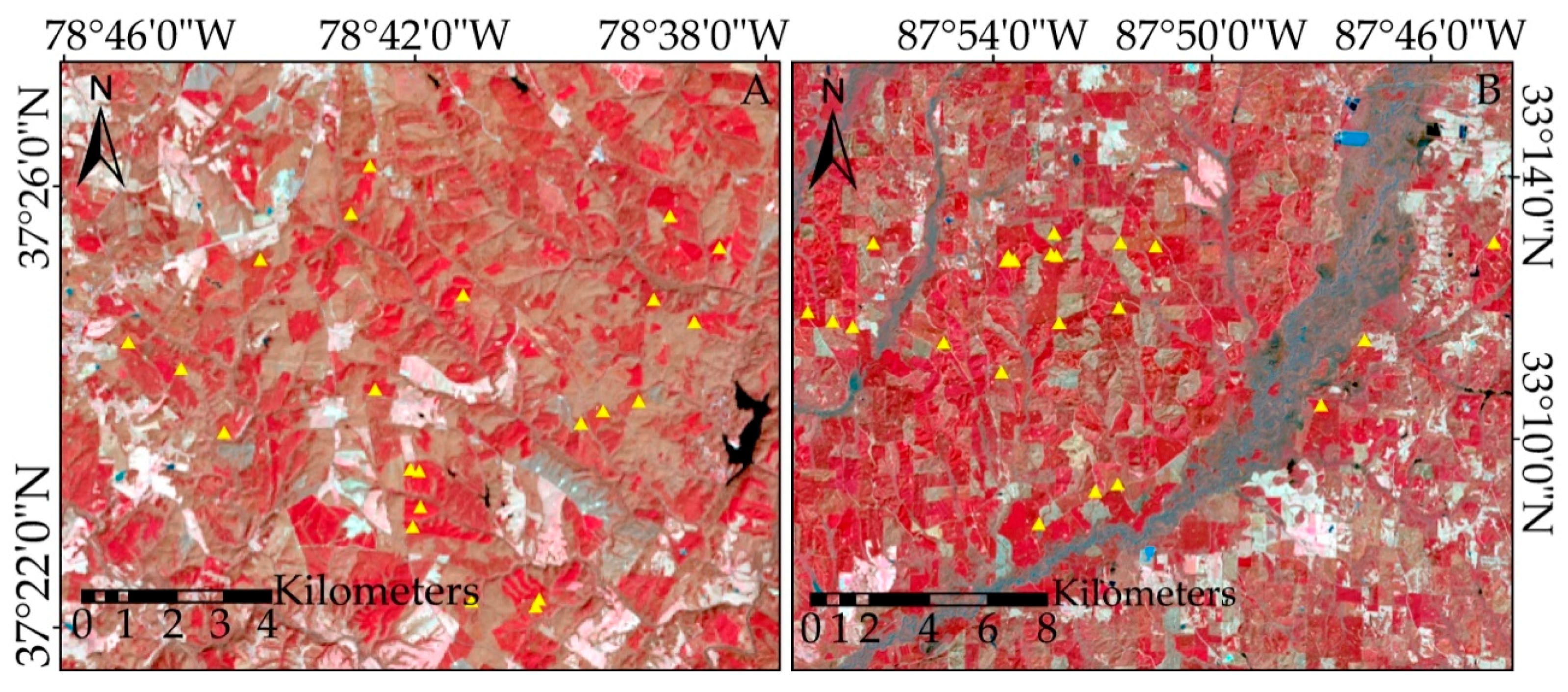
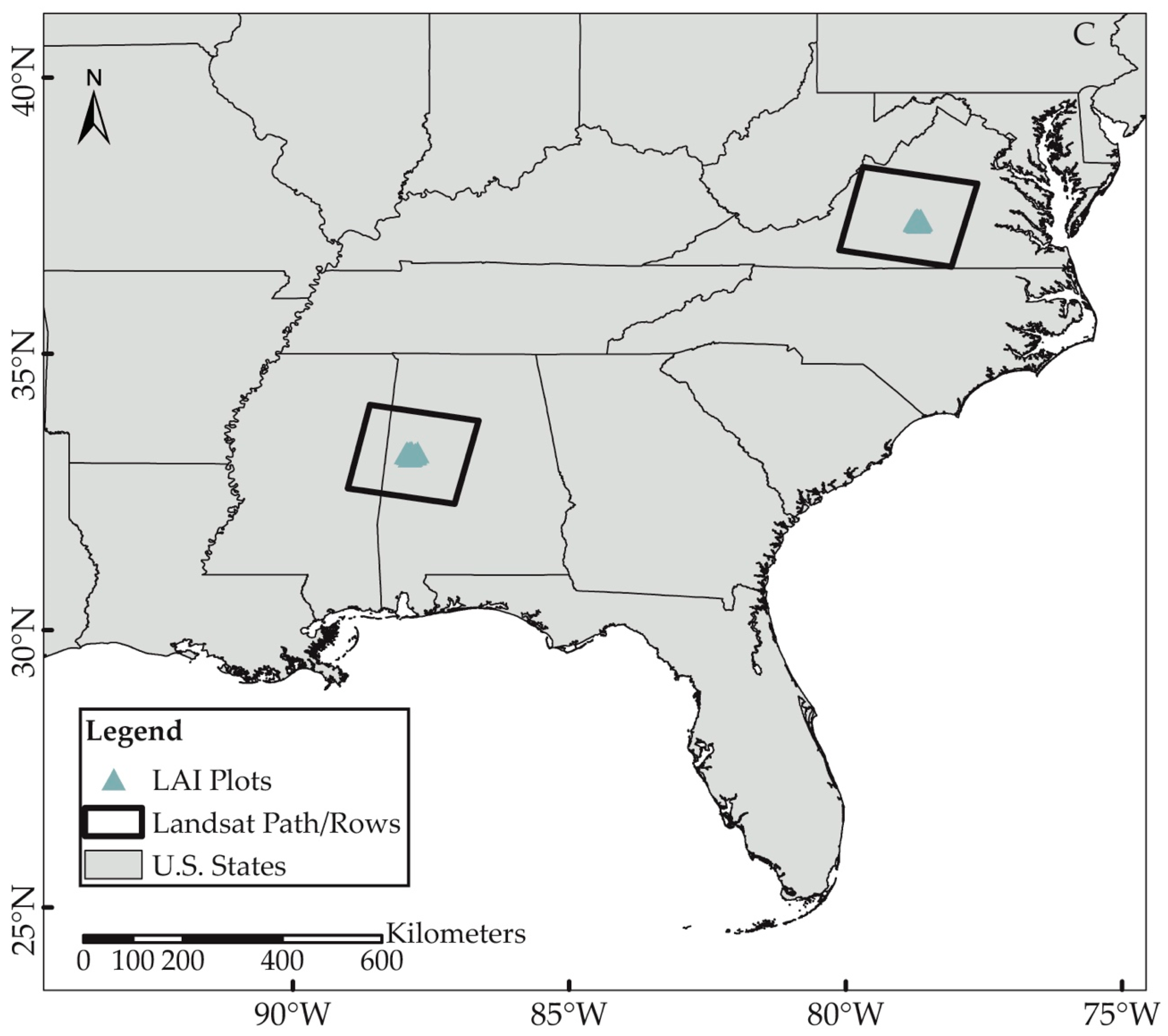
2.1. Study Sites and Field Data

Twenty-two permanent ground plots (Figure 1) were established in loblolly pine plantations at each of the two study sites (Figure 1C) for the estimation of ground LAI. One site was established at the Appomattox-Buckingham State Forest near Appomattox, Virginia, USA in March of 2013 which is within Landsat Worldwide Reference System 2 (WRS-2) path 16 row 34 (16/34). A second site was established on forest industry land near Tuscaloosa, AL in February of 2014 which is located in WRS-2 path 21 row 37 (21/37). The Virginia site is located in the Piedmont and the Alabama site is located in the Coastal Plain physiographic province. Pine stands were selected to cover the variability in LAI across the sites and to minimize the within stand variability of LAI. Each plot is 30 by 30 m in size (but not installed to align perfectly with a single pixel footprint) and all plot centers were established at least 30 m from stand boundaries. Very little to no evergreen understory existed within any of the ground LAI plots. A Trimble GeoXT was used to collect GPS locations for each plot center with the Trimble TerraSync software version 5.02. All GPS points were differentially corrected in Trimble’s GPS Pathfinder Office software version 5.20 to a horizontal accuracy of less than one meter.

Optical ground measurements of LAI were collected using two cross-calibrated LI-COR LAI-2200 or 2200C Plant Canopy Analyzers (and one data logger) with 90 degree view caps [28], cross-checked with litter traps and hemispheric photography in a prior study in this ecosystem [29]. The sensor was held at approximately 3.5 feet off the ground. One LAI-2200 sensor was set up in a large open area in close proximity to the ground plots to continuously collect above canopy readings at a 15 s interval during plot measurements. Both diagonals of each ground plot were sampled with at least 27 below canopy readings per plot. LAI sampling was predominantly conducted during relatively clear sky days or when the sky was uniformly overcast as recommended by LI-COR, Inc. (Lincoln, NE 68504, USA) [30]. LAI estimates for each below canopy reading were obtained using LI-COR’s FV2200 software version 2.0 or 2.1 with a horizontal model and the exclusion of ring 5, which is most highly obstructed by trunks and branches [16]. These LAI estimates might be better thought of as plant area index since anything including stems and branches that blocks the sensors view of incoming radiation impacts the estimates. Since the FV2200 software includes a correction for clumping (employed in this study), these estimates are closer to true LAI than effective LAI [30]. All LAI estimates for a given plot and measurement period were averaged and used as the dependent variables in subsequent analyses.

Plots were measured two times a year since installation in close proximity to maximum and minimum LAI (

Table 1. Ground LAI measurement details by study location (Virginia: 16/34, Alabama: 21/37) and LAI status (maximum or minimum). The maximum number of plots that were used in subsequent analyses is included in parentheses in column 4. Some plots were not used due to ground data errors and atmospheric conditions (clouds and shadows). Updated values are provided in parentheses in column 3 when the LAI range changed due to plot removal.

Location of LAI & Status	Ground Measurement Dates	Ground LAI Range (Min–Max)	Plots Measured (Max Used)	OLI Image Date	ETM+ Image Date
VA Min	1 April 2013 & 3 April 2013	1.14–3.07	22 (20)	28 March 2013	19 March 2013
VA Max	13 September 2013 & 14 September 2013	2.04–5.39 (5.33)	10 (8)	5 October 2013	11 September 2013
AL Min	21 February 2014, 24 February 2014 & 27 February 2014	0.68–4.42 (3.93)	22 (21)	13 February 2014	21 February 2014
VA Min	26 March 2014	1.13–4.39 (3.43)	19 (18)	14 March 2014	23 April 2014
AL Max	14 September 2014 & 25 September 2014	0.63–7.34 (5.14)	9 (7)	25 September 2014	1 September 2014
VA Max	20 September 2014	2.04–5.94 (5.60)	20 (19)	22 September 2014	29 August 2014

) resulting in six separate field data collections. Since LAI variations occur more rapidly in the growing season than in the winter, and there is often reduced image availability in the summer due to cloud cover, we attempted to match ground data collection as closely as logistically possible to image acquisition dates. LAI estimates for each ground plot at a given site from maximum and minimum LAI within a given year were plotted against one another to identify erroneous ground data points. For the VA site, interannual plots of minimum and maximum LAI were also created. Any plot from a given measurement period that was clearly outside realistic bounds (i.e., less than zero or greater than ten) was removed from the data set. For the thirteen plots with repeat measurements across three seasons, inter-season residual correlation never exceeded 0.31, well within the 95% threshold of 0.53. As such, error independence was assumed.

2.2. Landsat Data and LAI Regression Models

2.2.1. Landsat Sensors

The two different sensors used, Landsat 7 ETM+ and Landsat 8 OLI, have different band orders, as illustrated in

Table 2. Landsat sensors and specific bands used in VIs. All bands listed have a resolution of 30 m. This highlights the differences in wavelength of the bands between Landsat 7 and Landsat 8 [31].

Band Name	Landsat 7 ETM+ Band Number	Landsat 7 ETM+ Wavelength (Micrometers)	Landsat 8 OLI Band Number	Landsat 8 OLI Wavelength (Micrometers)
Blue	1	0.441–0.514	2	0.452–0.512
Red	3	0.631–0.692	4	0.636–0.673
Near Infrared (NIR)	4	0.772–0.898	5	0.851–0.879
Shortwave Infrared (SWIR) 1	5	1.547–1.749	6	1.566–1.651

. The imagery from Landsat 7 ETM+ is subject to the Scan Line Corrector (SLC) failure and one plot from the Virginia study site location fell within the resulting data gap, resulting in 21 available plots for ETM+ scenes.

From Landsat 7 ETM+ to Landsat 8 OLI, the wavelengths of the bands have changed. The OLI sensor’s bands are much narrower than the ETM+ bands as shown in Table 2. This improvement allows the OLI sensor to potentially experience less saturation within the bands and to avoid atmospheric absorption features to which ETM+ bands were subjected [32].

2.2.2. Vegetation Indices and Reflectance

Landsat ETM+ and OLI imagery from 16/34 and 21/37 with the least cloud cover (of the available dates near ground measurement dates) over the LAI plots and closest in time and phenological stage to the ground LAI measurement dates (Table 1) were ordered from the USGS ESPA ordering interface (https://espa.cr.usgs.gov/). The ETM+ Level-1 scenes were corrected to surface reflectance using the Landsat Ecosystem Disturbance Adaptive Processing System (LEDAPS) and all OLI scenes were corrected to surface reflectance using the Landsat 8 Surface Reflectance Code (LaSRC) algorithm [31]. Both top-of-atmosphere (TOA) and bottom-of-atmosphere (surface) reflectance data were obtained. VIs available through the ESPA Ordering Interface, including normalized difference vegetation index (NDVI), enhanced vegetation index (EVI), soil adjusted vegetation index (SAVI), modified soil adjusted vegetation index (MSAVI), and normalized difference moisture index (NDMI), were obtained or calculated for surface reflectance for each image date [31] (see equations below). The simple ratio (SR) vegetation index was also calculated using ESRI’s ArcGIS 10.2 for Desktop’s raster calculator for both TOA and surface reflectance for each image date. One OLI image was collected on 28 March 2013 over the VA study area for 16/34 before Landsat 8 reached final WRS-2 orbit and was not available through the ESPA site. This image was processed to TOA reflectance and used in subsequent analyses. Each index below explains which bands of each sensor are used in the equation.

Normalized Difference Vegetation Index [33]:

$$\mathrm{NDVI}=\frac{{\mathsf{\rho }}_{NIR}-{\mathsf{\rho }}_{Red}}{{\mathsf{\rho }}_{NIR}+{\mathsf{\rho }}_{Red}}$$

(1)

where ${\mathsf{\rho }}_{NIR}$ is the reflectance in the near infrared band (band 4 with ETM+ and band 5 with OLI) and ${\mathsf{\rho }}_{Red}$ is the red band reflectance (band 3 with ETM+ and band 4 with OLI).

Enhanced Vegetation Index [34]:

$$\mathrm{EVI}=\frac{{\mathsf{\rho }}_{NIR}-{\mathsf{\rho }}_{Red}}{\left({\mathsf{\rho }}_{NIR}+C_1{\ast \mathsf{\rho }}_{Red}-C_2{\ast \mathsf{\rho }}_{Blue}+L\right)}$$

(2)

where ${\mathsf{\rho }}_{Blue}$ is the reflectance in the blue band (band 1 with ETM+ and band 2 with OLI), L is an adjustment for canopy background and set to 1 for both sensors, and $C_1$ and $C_2$ are coefficients for atmospheric resistance. $C_1$ = 6 and $C_2$ = 7.5 for both ETM+ and OLI.

Soil Adjusted Vegetation Index [35]:

$$\mathrm{SAVI}=\frac{\left({\rho }_{NIR}-{\rho }_{Red}\right)\left(1+L\right)}{{\rho }_{NIR}+{\rho }_{Red}+L}$$

(3)

where L is a soil brightness correction factor that is set to 0.5 for both ETM+ and OLI.

Modified Soil Adjusted Vegetation Index [36]:

$$\mathrm{MSAVI}=\frac{2\left({\rho }_{NIR}+1\right)-\sqrt{{\left(2{\rho }_{NIR}+1\right)}^2-8\left({\rho }_{NIR}-{\rho }_{Red}\right)}}{2}$$

(4)

Normalized Difference Moisture Index [37]:

$$\mathrm{NDMI}=\frac{{\rho }_{NIR}-{\rho }_{SWIR1}}{{\rho }_{NIR}+{\rho }_{SWIR1}}$$

(5)

where ${\rho }_{SWIR1}$ is the reflectance in the shortwave infrared band (band 5 with ETM+ and band 6 with OLI.

Simple Ratio:

$$\mathrm{SR}=\frac{{\rho }_{NIR}}{{\rho }_{Red}}$$

(6)

2.2.3. LAI Regression Models

Simple linear regression models were calculated using the ground LAI estimates from a given site, year, and time period (minimum or maximum LAI) as the dependent variable and SR calculated with either TOA reflectance or surface reflectance as the independent variable. (Only SR was used for the comparison of TOA and surface reflectance, since SR is the only VI used in the current operational standard [15]). For the TOA and surface reflectance comparison, separate models were created for a single measurement period/site. Combinations of the ground measurements, including all maximum LAI, all minimum LAI, and both maximum and minimum LAI combined (the combined model), were compared across all VIs and for TOA- and surface reflectance-based SR models. Plots that either fell inside ETM+ data gaps or that were impacted by clouds or cloud shadows in a given image were excluded from the data set, as indicated in Table 1. Bootstrap statistics for the best overall model were computed with 100,000 replicates using the boot package (version 1.3–20) in R (version 3.5.1 “Feather Spray”). Bootstrap confidence intervals were calculated using boot.ci with 100,000 replicates and the adjusted bootstrap percentile method (type = “bca”).

2.2.4. Georegistration Accuracy

To determine if the georegistration accuracy of OLI images had any impact on the LAI regression results, each set of ground plots at the two study sites were shifted to the location of one of their 8 neighbors. For each of the 8 sets of locations, the SR vegetation index based on TOA reflectance were extracted and used in regression models. For example, all of the plots at the VA study site were shifted up one pixel, the SR pixel values at these new locations were then extracted for each plot and used as the independent variable in a regression model with the ground plot LAI estimates. This was repeated for each of the remaining 7 pixel locations in a 3 by 3 window around the plot center pixel. The regression results from the 8 neighboring pixels were then compared with those of the plot center pixel. These calculations were made using one OLI image date (Table 1) for each set of ground LAI data.

2.2.5. Comparison to Current Operational Standard

To assess whether our updated model has potential to replace the one in common operational use, we mapped LAI with our updated combined SR model and with the model presented by Flores et al., commonly used for pine silviculture decision support in the U.S. South (Equation (7)) [15].

$$\mathrm{LAI}=0.56\mathrm{SR}-0.83$$

(7)

Two scenes were acquired covering the Appomattox Buckingham State Forest in Virginia, one for maximum and one for minimum LAI. The scenes were from the analysis ready data Landsat 8 data products and the bottom-of-atmosphere (surface) reflectance was retained for subsequent analysis. SR was derived for each image and each image was clipped to the shape of the Appomattox Buckingham State Forest. The two empirical models were then calculated for each pixel within the state forest.

3. Results

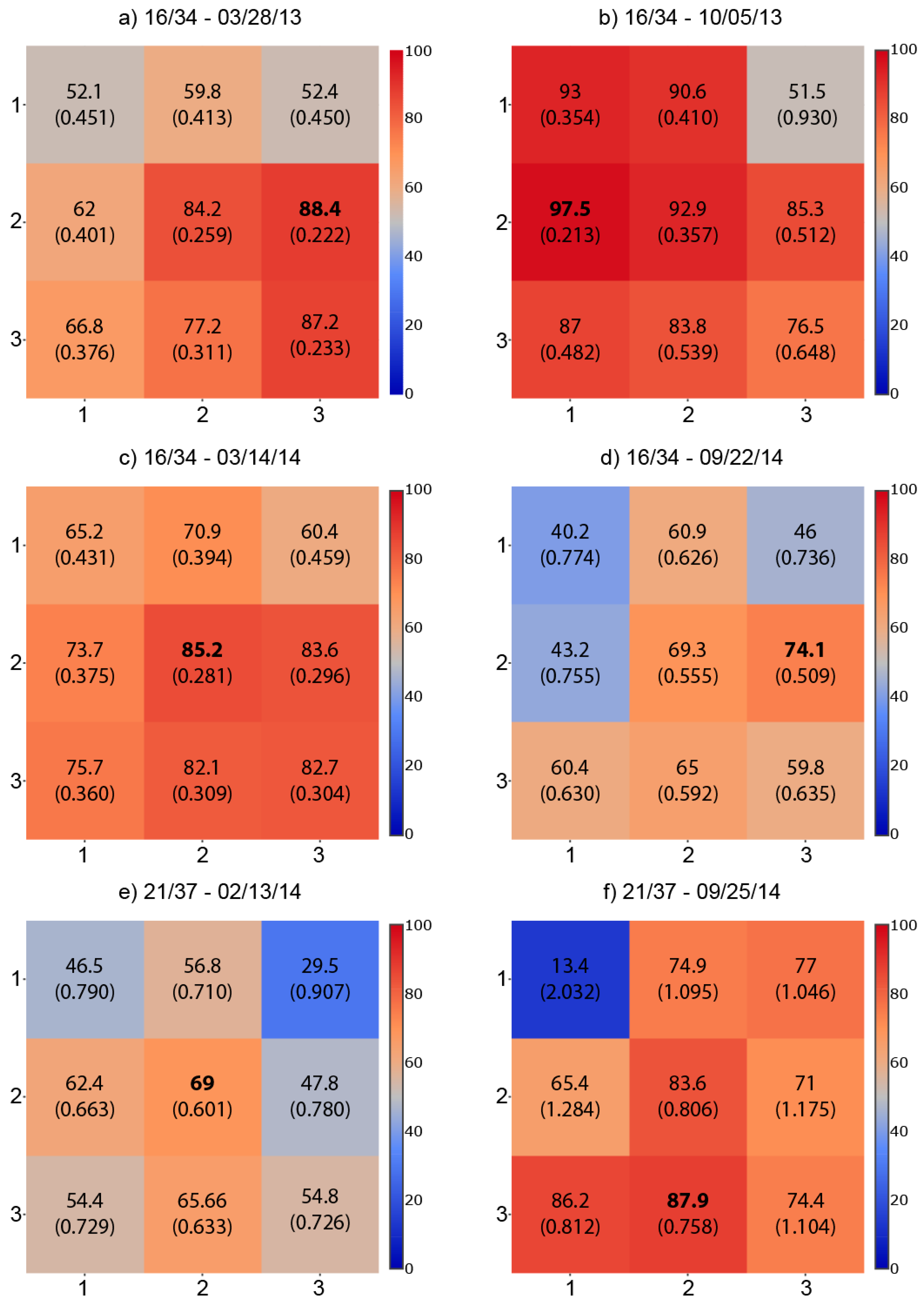
3.1. Georegistration Impacts

The 16/34 image acquired on 14 March 2014 (Figure 2c) and 21/37 image acquired on 13 February 2014 (Figure 2e) resulted in the best LAI regression model with the plot center pixel (Figure 2). There was not a consistent trend in terms of which adjacent pixel resulted in the most accurate LAI model with the four other images (Figure 2a,b,d,f). In every instance, at least one of the adjacent pixels to the plot centers resulted in models that explained significantly less of the variability within the ground measurements (Figure 2). Accurate plot and pixel locations are clearly a critical component of model development with any combination of ground and remotely-sensed measurements.

3.2. TOA versus Surface Reflectance

Regression results for the SR models comparing surface to TOA reflectance are shown in

Table 3. Regression results between ground measured LAI and Landsat OLI TOA- and surface reflectance-based SR (bold R²s denote the regression with the best fit for the given ground data collection). * These plot numbers are just for TOA reflectance since the surface reflectance plot numbers were reduced to 39 and 73 for minimum and combined, respectively, due to the surface reflectance image of one 16/34 image date being unavailable.

Path/Row Time Period	Closest OLI Date	OLI R-sq (RMSE) TOA	OLI R-sq (RMSE) Surface	Min/Max R-sq (RMSE) TOA	Combined R-sq (RMSE) TOA	Min/Max R-sq (RMSE) Surface	Combined R-sq (RMSE) Surface	Max Number of Plots Used Separate/Min or Max/Combined
16/34 2013 Min	28 March 2013	84.2 (0.259)	N/A	67.8 (0.468)	73.2 (0.641)	73.3 (0.472)	78.7 (0.613)	19/58 */92 *
21/37 2014 Min	13 February 2014	69.0 (0.601)	76.1 (0.528)					21/58 */92 *
16/34 2014 Min	14 March 2014	85.2 (0.281)	84.7 (0.285)					18/58 */92 *
16/34 2013 Max	5 October 2013	92.9 (0.357)	92.1 (0.376)	58.6 (0.840)		68.7 (0.730)		8/34/92 *
16/34 2014 Max	22 September 2014	69.3 (0.555)	66.0 (0.584)					19/34/92 *
21/37 2014 Max	25 September 2014	86.4 (0.806)	90.8 (0.663)					7/34/92 *

. Surface reflectance resulted in models that were more accurate for the individual measurement periods with the Alabama study area (21/37) while TOA reflectance outperformed surface reflectance at the Virginia study area. While TOA reflectance showed better results than surface reflectance three out of five times with the ground data from individual measurement periods, surface reflectance showed better results for each of the combined ground data sets, minimum LAI, maximum LAI and combined LAI (

Table 4. Bootstrap statistics (100,000 replicates) for best overall regression model. CI = 95% confidence interval.

	Original	Bias	Standard Error	Lower CI	Upper CI
Intercept	−0.002119728	0.0004935929	0.13349108	−0.2755	0.2498
Slope	0.332915393	−0.0001120626	0.01585535	0.3021	0.3646

). If the VA minimum LAI 2013 plots are excluded from the TOA analysis, the R² s and RMSEs change to 72.4 (0.480) for TOA minimum LAI and 73.5 (0.682) for TOA combined LAI, which are still not as good as the surface reflectance results (Table 4).

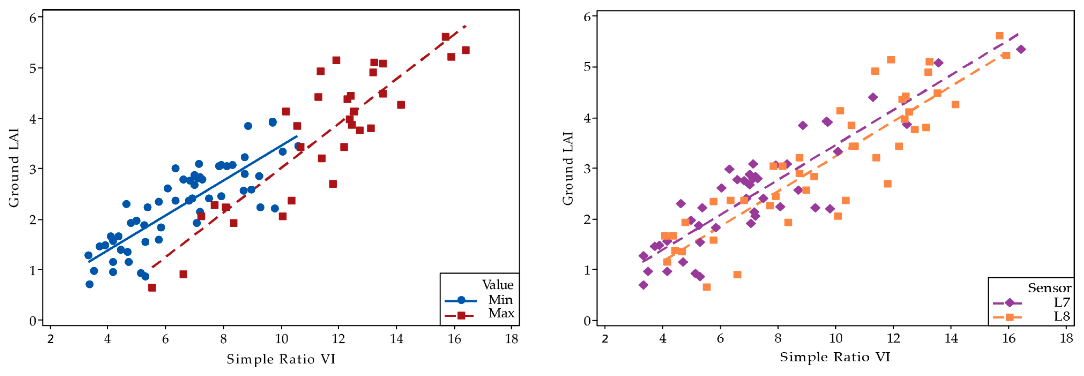
3.3. Vegetation Indices Comparison

NDMI resulted in the most accurate LAI model for six of the nine combinations of LAI time period and sensor considered with the SR vegetation index being most accurate three out of nine times (Table 4). NDVI, EVI, SAVI and MSAVI never resulted in the most accurate LAI model out of the six VIs considered. Unlike EVI, SAVI and MSAVI, NDVI produced the second most accurate model seven out of nine times. NDMI resulted in the best model for all time periods with the ETM+ sensor and for all of the maximum LAI models regardless of sensor (Table 4). Landsat OLI produced the most accurate LAI model for a given time period two out of three times with the SR vegetation index. SR also resulted in the best all time periods model two out of three times. For five of the nine time-period and sensor combinations, NDVI yielded a more accurate model than SR. NDMI, NDVI and SR always produced more accurate LAI models than EVI, SAVI and MSAVI for a given ground data set (time period) across sensors when calculated with surface reflectance. Using the closest in time image to the ground data collection regardless of sensor (the “Both” sensor option in Table 4) resulted in more accurate LAI models than using data from either of the sensors separately.

3.4. LAI Model

Equation (8) is the best regression model for ground data from all time periods and VIs from both sensors (see also Figure 3; Table 4 and

Table 5. Regression results between ground measured LAI and Landsat surface reflectance-based VIs (bold R²s denote the regression with the best fit for the given time period and Landsat sensor). * These results do not include an OLI image for the VA study site at minimum LAI in 2013.

Time Period	Landsat Sensor	NDMI R2 (RMSE)	NDVI R2 (RMSE)	SR R2 (RMSE)	EVI R2 (RMSE)	MSAVI R2 (RMSE)	SAVI R2 (RMSE)	Number of Plots
Minimum *	OLI	66.6	70.8	73.3	62.6	59.8	62.8	39
		(0.528)	(0.494)	(0.472)	(0.558)	(0.579)	(0.557)
Maximum	OLI	80.7	69.5	68.7	48.3	47.0	49.0	34
		(0.573)	(0.721)	(0.730)	(0.939)	(0.951)	(0.933)
All	OLI	65.9	69.2	78.7	58.2	56.6	58.5	73
		(0.774)	(0.736)	(0.613)	(0.858)	(0.874)	(0.854)
Minimum	ETM+	72.4	65.3	63.6	55.6	56.3	59.4	56
		(0.432)	(0.485)	(0.496)	(0.548)	(0.544)	(0.524)
Maximum	ETM+	81.1	60.0	49.3	65.7	65.5	66.7	26
		(0.582)	(0.847)	(0.954)	(0.784)	(0.786)	(0.772)
All	ETM+	74.2	65.6	67.1	64.2	65.0	65.0	82
		(0.605)	(0.698)	(0.684)	(0.713)	(0.705)	(0.704)
Minimum	Both	74.5	69.8	69.4	63.8	58.4	60.7	57
		(0.415)	(0.452)	(0.455)	(0.494)	(0.530)	(0.515)
Maximum	Both	82.8	77.8	77.2	32.0	38.8	41.3	32
		(0.554)	(0.630)	(0.639)	(1.103)	(1.046)	(1.025)
All	Both	73.3	68.9	79.2	57.2	57.9	59.0	89
		(0.635)	(0.686)	(0.561)	(0.805)	(0.799)	(0.788)

).

$$\mathrm{LAI}=0.332915\mathrm{SR}-0.00212$$

(8)

The regression differences between using only maximum versus only minimum and of OLI (L8) versus ETM+ (L7) are shown as Figure 4.

3.5. Comparison to Current Operational Standard

The sample data used to derive the Flores et al. model do not have as wide a range as the sample data used to derive our combined model using SR as shown in Figure 5 [15].

Flores et al. [15] found when using winter scenes, when phenological differences are minimized, LAI of loblolly pine plantations could be accurately estimated using Landsat-derived SR [15]. Using summer scenes exclusively has not resulted in robust LAI models. However, when both maximum and minimum LAI data are combined the results are better than using the data from winter alone, as shown in Table 4. By using winter data exclusively in model development, LAI may be overestimated when estimating maximum LAI as shown in Figure 6 and Figure 7. It should also be noted that the model from Flores et al. [12] was developed using TOA rather than surface reflectance and measured many fewer plots in situ. The Flores et al. [15] model has a large number of values that are considered to be overly high (above seven) for the species at this site (Figure 7). In our combined model, there are very few LAI values above seven, another indication of its potential utility for operational use.

4. Discussion

4.1. Georegistration Impacts

Landsat misregistration is a source of error for studies assessing change through time [38] or relating plot-level to satellite-derived measurements [39]. McRoberts et al. [39] note that “for common magnitudes of rectification and GPS errors, as many as half the ground plots may be assigned to incorrect pixels.” With these and related studies in mind, the size of the LAI ground plots in this study was selected to match the size of a Landsat pixel with the goal of improving the relationship between the ground and satellite data. However, the ground plots were not installed to align perfectly with a single pixel footprint. This is why stands that were as homogeneous as possible with respect to LAI were used and plot locations were selected in areas with similar LAI estimates in the surrounding 3 × 3 pixel area as illustrated in Figure 2. Plots were also located at least 30 m from a stand boundary to avoid having the plot center fall inside a mixed pixel. Additionally, the LAI-2200 measured beyond the plot boundaries when readings were collected in close proximity to the plot boundaries, as they were at the start and end of each transect. A relatively large number of LAI-2200 readings were collected per plot transect to improve the estimated ground LAI values for a given plot and to minimize the impact of any single erroneous readings. The geometric accuracy requirement for OLI is 12 m (less than half the width of the ground resolution cell size), met or exceeded in operations [40]. Furthermore, the Thematic Mapper, ETM+, and OLI all exceed the 12 m geometric accuracy requirement at least 92% of the time [41]. This realized geometric accuracy requirement, coupled with careful plot placement and submeter GPS accuracy, was sufficient to relate ground- to satellite-derived measurements on a pixel-specific basis (Figure 2).

4.2. TOA versus Surface Reflectance

Both TOA and surface reflectance performed well across models. However, with the combined data sets, surface reflectance (R² = 78.7%) outperformed TOA reflectance (R² = 73.2%), as shown in Table 3. Surface reflectance also performed better than TOA reflectance across three sensors (IKONOS, SPOT, and ETM+) in the Soudani et al. [42] study. A recent study [43] comparing Landsat TOA and surface reflectances to estimate the fraction of absorbed photosynthetically active radiation (FPAR; physiologically related to LAI) found that surface reflectance also slightly outperformed TOA reflectance (surface reflectance error, 0.03; TOA reflectance error, 0.06). Our results, in conjunction with the prior literature, strongly suggest that Landsat surface reflectance data be used for empirical LAI estimation.

4.3. Vegetation Indices Comparison

The relationships between VIs and LAI remained linear (and thus did not saturate) at any field-measured LAI value in this study, unlike many that preceded it. Some field LAI estimates exceeded 5 (Table 1). Chen et al. [44] did not find a saturation point at high LAI in boreal conifer stands and also found the relationship between optical ground LAI estimates and the Landsat SR to be linear in the summer. Data measured across multiple Landsat path/rows were also combined were found necessary to develop reliable models [44]. Similarly, Potithep et al. [27] found a two-period relationship better than a single period between in situ LAI estimates and in situ VIs derived from a hemispherical spectroradiometer in a deciduous forest. Although our combined data did not result in a better fit than the single image models, they did have strong relationships (Table 3) and the combined model across sites and times has greater utility for forest managers.

Cohen et al. [45] also advocated for the use of VIs from multiple dates of imagery in regression analyses for the estimation of LAI. Exploration of more than one spectral variable or VI in the LAI regression models may be warranted in future work based on the findings of [45] and Fassnacht et al. [46]. Evaluation of LAI estimates for a given site at two points in time close to minimum and maximum LAI was also explored by [25] in mixed natural forests in the southeastern U.S.

Dube and Mutanga [47] showed that texture parameters could enhance aboveground biomass estimation in deciduous forests. Since Madugundu et al. [48] previously noted a strong relationship between aboveground biomass and LAI in both pine and eucalyptus plantations, it follows that texture might also improve LAI models. However, Gray and Song [49] mapped minimum and maximum LAI by combining the spectral, spatial and temporal information of Landsat, IKONOS and MODIS, respectively, but did not find a significant relationship between texture variables and effective LAI in evergreen stands. Since (1) texture variables are neighborhood-derived variables and are thus less useful for sub-stand, pixel-specific estimates; and (2) they have not yet been directly shown to be useful for LAI estimation in pines, we did not employ them in this study. However, it seems prudent that future studies focused on stand-scale LAI estimation consider texture parameters as predictor variables.

Chen et al. [50] found that when using multiple sensors, the ones that had a larger discrepancy between plot size and sensor resolution did not perform as well as the sensors that were closer to the plot size. Middinti et al. [51] found that when combining MODIS and OLI data there were a significant number of high LAI values when compared to a solely OLI-derived map. This supports the notion that the larger the sensor resolution difference when combining multiple sensor types, the less apt the combination is at estimating LAI. Korhonen et al. [52] compared Sentinel 2 to Landsat 8 and found that when using conventional indices, the sensors performed similarly (for scale-appropriate analyses).

Similar to our results, SAVI and EVI (both of which contain the blue band, which is often more difficult to convert to surface reflectance) did not perform well in comparison to NDVI and SR for the estimation of LAI in Scots pine stands [42]. Lee et al. [53] compared hyperspectral and multispectral data for LAI estimation and found bands in the red-edge and shortwave-infrared regions to be more important than near-infrared bands. Similarly, Eklundh et al. [54] found both SWIR1 and SWIR2 more correlated with boreal pine LAI than any other ETM+ spectral channel. This might partially explain why NDMI, which uses a shortwave infrared band, outperformed both NDVI and simple ratio a majority of the time in this study (Table 5). This echoes the results of Eklundh [55] who found the moisture stress index (SWIR1 − NIR) the best index, out of many tested, for coniferous stands. Further, Kodar et al. [56] found NDVI to be the worst performing of all tested VIs for boreal LAI estimation.

Tillack et al. [26] looked at seasonal relationships between ground LAI estimates and high-resolution VIs from RapidEye. The strength of the relationships and the VI that produced the strongest relationships varied with the seasons, but NDVI worked best when all seasons were combined. In this study, simple ratio and NDMI worked best when minimum and maximum LAI were combined. Like [26], our field data only measured the LAI stand component above the sensor which was held at approximately 3.5 feet off the ground and above any low understory vegetation. The exclusion of portions of the understory LAI in our maximum LAI ground estimates likely causes some of the unexplained variation in our models, especially in areas with incomplete canopy closure.

4.4. LAI Model

This study’s combined model used data from both Landsat 7 ETM+ and Landsat 8 OLI. Flores et al. [15] used Landsat 7 ETM+ exclusively. Masemola et al. [57] found, when comparing Landsat 7 ETM+ to Landsat 8 OLI data, that Landsat 8 OLI estimated grass LAI with better accuracy than Landsat 7 ETM+. Through the use of a combined radiative transfer model (one-dimensional leaf reflectance, PROSPECT and a canopy reflectance model, SAIL) called PROSAILH, they found Landsat 8 OLI data showed significant improvement over Landsat 7 ETM+ data and concluded that OLI data could be used to accurately estimate LAI when compared to ETM+. When estimating LAI, Schott et al. [58] found that regression model fits improved with the increase in signal-to-noise ratio from ETM+ imagery to OLI imagery and that the increases in signal-to-noise ratio were significant.

Time between the ground data collection and image acquisition is clearly an important factor in the estimation of LAI. Although the OLI sensor has a number of improvements [59] over the ETM+ sensor, timing mattered more than the sensor in this study. Similarly, Zhang et al. [60] found that an estimated Landsat VI based on MODIS fusion that matched the date of the summer ground LAI estimates from a study site in Canada resulted in better LAI models than the three available cloud free Landsat images that were collected 17 or more days before or after the ground data. Since LAI variations occur more rapidly in the growing season than in the winter, and there is often reduced image availability in the summer due to cloud cover, these findings are not surprising. For this reason, we attempted to match ground data collection as closely as logistically possible to image acquisition dates. Since both ETM+ and OLI data can be used effectively for LAI estimation, a given site has the potential of a good Landsat image every 8 days instead of 16 days. Based on this, future studies should focus on acquiring ground LAI estimates on or within a few days of image acquisition.

4.5. Comparison to Current Operational Standard

The model from Flores et al. [15] (Equation (7)) used as the current operational standard was derived using TOA reflectance data in concert with in situ data from a fertilization study at a unique site (SETRES-2) on the North Carolina coastal plain. By using both fertilized and control plots across differing soil conditions they compiled 12 observations, which resulted in no observed LAI in the winter between 1.75 and 2.5 [15]. Our study used two different regions in the southeastern United States (industry land in Alabama and managed state forest in Virginia) across two years and included two winter and two summer seasons. By expanding to two regions, multiple years, and multiple sensors, we were able to include 89 observations to derive our model, which used surface rather than TOA reflectance. More than a third of our winter LAI data fell between 1.75 and 2.5. The fact that this study had more samples over a wider range of LAI than that of Flores et al. [15] likely improved the robustness of the resulting model. Qualitatively, as seen in Figure 6 and Figure 7, the resulting mapped estimates are more realistic with the new model than with the current operational standard.

5. Conclusions

This study has shown that ground LAI estimates at minimum and maximum LAI in loblolly pine stands can be combined and modeled with Landsat VIs across sites and sensors. SR and NDMI both produce strong relationships with LAI data combined across seasons. Collecting ground data in close proximity to image acquisition has a greater influence on LAI-VI modeling than Landsat sensor does. Data from both current Landsat sensors, ETM+ and OLI, can be combined and used in the same model. Accurate plot and pixel locations are important for minimizing unexplained variability within LAI-VI models. The resulting combined model using SR is recommended for operational use in the southeastern USA.

References

1. Rubilar, R.A.; Lee Allen, H.; Fox, T.R.; Cook, R.L.; Albaugh, T.J.; Campoe, O.C. Advances in silviculture of intensively managed plantations. Curr. For. Rep. 2018, 4, 23–34. [Google Scholar] [CrossRef]
2. Allen, H.L.; Fox, T.R.; Campbell, R.G. What is ahead for intensive pine plantation silviculture in the South? South. J. Appl. For. 2005, 29, 62–69. [Google Scholar]
3. Osem, Y.; O’Hara, K. An ecohydrological approach to managing dryland forests: Integration of leaf area metrics into assessment and management. Forestry 2016, 89, 338–349. [Google Scholar] [CrossRef]
4. Sampson, D.A.; Amatya, D.M.; Lawson, C.D.B.; Skaggs, R.W. Leaf area index (LAI) of loblolly pine and emergent vegetation following a harvest. Trans. ASABE 2011, 54, 2057–2066. [Google Scholar] [CrossRef]
5. Fox, T.R.; Allen, L.H.; Albaugh, T.J.; Rubilar, R.; Carlson, C.A. Tree nutrition and forest fertilization of pine plantations in the southern United States. South. J. Appl. For. 2007, 31, 5–11. [Google Scholar]
6. Albaugh, T.J.; Allen, H.L.; Dougherty, P.M.; Kress, L.W.; King, J.S. Leaf area and above- and belowground growth responses of loblolly pine to nutrient and water additions. For. Sci. 1998, 44, 317–328. [Google Scholar]
7. Campoe, O.C.; Stape, J.L.; Albaugh, T.J.; Allen, H.L.; Fox, T.R.; Rubilar, R.; Binkley, D. Fertilization and irrigation effects on tree level aboveground net primary production, light-interception and light use efficiency in loblolly pine plantation. For. Ecol. Manag. 2013, 288, 43–48. [Google Scholar] [CrossRef]
8. Samuelson, L.J.; Pell, C.J.; Stokes, T.A.; Bartkowiak, S.M.; Akers, M.K.; Kane, M.; Markewitz, D.; McGuire, M.A.; Teskey, R.O. Two-year throughfall and fertilization effects on leaf physiology and growth of loblolly pine in the Georgia Piedmont. For. Ecol. Manag. 2014, 330, 29–37. [Google Scholar] [CrossRef]
9. Blinn, C.E.; Albaugh, T.J.; Fox, T.R.; Wynne, R.H.; Stape, J.L.; Rubilar, R.A.; Allen, H.L. A method for estimating deciduous competition in pine stands using Landsat. South. J. Appl. For. 2012, 36, 71–78. [Google Scholar] [CrossRef]
10. Gonzalez-Benecke, C.A.; Jokela, E.J.; Martin, T.A. Modeling the effects of stand development, site quality, and silviculture on leaf area index, litterfall, and forest floor accumulation in loblolly and slash pine plantations. For. Sci. 2012, 58, 457–471. [Google Scholar] [CrossRef]
11. Gao, F.; Anderson, M.C.; Kustas, W.P.; Houborg, R. Retrieving leaf area index from Landsat using MODIS LAI products and field measurements. IEEE Geosci. Remote Sens. 2014, 11, 773–777. [Google Scholar]
12. Vogel, S.A.; McKelvey, K.; Gholz, H.L.; Curran, P.J.; Ewel, K.C.; Cropper, W.P.; Teskey, R.O. Dynamics of canopy structure and light interception in Pinus elliottii stands, north Florida. Ecol. Monogr. 2006, 61, 33–51. [Google Scholar]
13. Sampson, D.A.; Albaugh, T.J.; Johnsen, K.H.; Allen, H.L.; Zarnoch, S.J. Monthly leaf area index estimates from point-in-time measurements and needle phenology for Pinus taeda. Can. J. For. Res. 2003, 33, 2477–2490. [Google Scholar] [CrossRef]
14. Eriksson, H.M.; Eklundh, L.; Kuusk, A.; Nilson, T. Impact of understory vegetation on forest canopy reflectance and remotely sensed LAI estimates. Remote Sens. Environ. 2006, 103, 408–418. [Google Scholar] [CrossRef]
15. Flores, F.J.; Allen, H.L.; Cheshire, H.M.; Davis, J.M.; Fuentes, M.; Kelting, D. Using multispectral satellite imagery to estimate leaf area and response to silvicultural treatments in loblolly pine stands. Can. J. For. Res. 2006, 36, 1587–1596. [Google Scholar] [CrossRef]
16. Peduzzi, A.; Allen, H.L.; Wynne, R.H. Leaf area of overstory and understory in pine plantations in the Flatwoods. South. J. Appl. For. 2010, 34, 154–160. [Google Scholar]
17. Iiames, J.S.; Congalton, R.G.; Pilant, A.N.; Lewis, T.E. Leaf area index (LAI) change detection analysis on loblolly pine (Pinus taeda) following complete understory removal. Photogramm. Eng. Remote Sens. 2008, 74, 1389–1400. [Google Scholar] [CrossRef]
18. Curran, P.J.; Dungan, J.L.; Gholz, H.L. Seasonal LAI in slash pine estimated with Landsat TM. Remote Sens. Environ. 1992, 39, 3–13. [Google Scholar] [CrossRef]
19. Chen, J.M.; Cihlar, J. Retrieving leaf area index of boreal conifer forests using Landsat TM images. Remote Sens. Environ. 1996, 55, 153–162. [Google Scholar] [CrossRef]
20. Tian, Q.; Luo, Z.; Chen, J.M.; Chen, M.; Hui, F. Retrieving leaf area index for coniferous forest in Xingguo County, China with Landsat ETM+ images. J. Environ. Manag. 2007, 85, 624–627. [Google Scholar] [CrossRef] [PubMed]
21. Franklin, S.E.; Lavigne, M.B.; Deuling, M.J.; Wulder, M.A.; Hunt, E.R. Estimation of forest leaf area index using remote sensing and GIS data for modelling net primary production. Int. J. Remote Sens. 1997, 18, 3459–3471. [Google Scholar] [CrossRef]
22. Turner, D.P.; Cohen, W.B.; Kennedy, R.E.; Fassnacht, K.S.; Briggs, J.M. Relationships between leaf area index and Landsat TM spectral vegetation indices across three temperate zone sites. Remote Sens. Environ. 1999, 70, 52–68. [Google Scholar] [CrossRef]
23. Song, C.H. Optical remote sensing of forest leaf area index and biomass. Prog. Phys. Geogr. 2013, 37, 98–113. [Google Scholar] [CrossRef]
24. Sumnall, M.; Peduzzi, A.; Fox, T.R.; Wynne, R.H.; Thomas, V.A.; Cook, B. Assessing the transferability of statistical predictive models for leaf area index between two airborne discrete return LiDAR sensor designs within multiple intensely managed loblolly pine forest locations in the south-eastern USA. Remote Sens. Environ. 2016, 176, 308–319. [Google Scholar] [CrossRef]
25. Pu, R.L. Mapping leaf area index over a mixed natural forest area in the flooding season using ground-based measurements and Landsat TM imagery. Int. J. Remote Sens. 2012, 33, 6600–6622. [Google Scholar] [CrossRef]
26. Tillack, A.; Clasen, A.; Kleinschmit, B.; Förster, M. Estimation of the seasonal leaf area index in an alluvial forest using high-resolution satellite-based vegetation indices. Remote Sens. Environ. 2014, 141, 52–63. [Google Scholar] [CrossRef]
27. Potithep, S.; Nagai, S.; Nasahara, K.N.; Muraoka, H.; Suzuki, R. Two separate periods of the LAI-VIs relationships using in situ measurements in a deciduous broadleaf forest. Agric. For. Meteorol. 2013, 169, 148–155. [Google Scholar] [CrossRef]
28. Welles, J.M.; Norman, J.M. Instrument for indirect measurement of canopy architecture. Agron. J. 1991, 83, 818–825. [Google Scholar] [CrossRef]
29. Peduzzi, A.; Wynne, R.H.; Fox, T.R.; Nelson, R.F.; Thomas, V.A. Estimating leaf area index in intensively managed pine plantations using air- borne laser scanner data. Forest Ecol. And Mgmt. 2012, 270, 54–65. [Google Scholar] [CrossRef]
30. LI-COR, Inc. LAI-2200C Plant Canopy Analyzer Instructions Manual; Publication Number 984-14112; LI-COR, Inc.: Lincoln, NE, USA, 2013. [Google Scholar]
31. USGS. Product Guide: Landsat Surface Reflectance-Derived Spectral Indices Version 2.6. Available online: landsat.usgs.gov/documents/si_product_guide.pdf (accessed on 12 April 2015).
32. Irons, J.R.; Dwyer, J.L.; Barsi, J.A. The Next Landsat Satellite: The Landsat Data Continuity Mission. Remote Sens. Environ. 2012, 122, 11–21. [Google Scholar] [CrossRef]
33. Rouse, J.W., Jr.; Haas, R.H.; Deering, D.W.; Schell, J.A.; Harlan, J.C. Monitoring the Vernal Advancement and Retrogradation (Green Wave Effect) of Natural Vegetation, NASA/GSFC Type III Final Report; Texas A&M University: College Station, TX, USA, 1974; 371p. [Google Scholar]
34. Huete, A.; Didan, K.; Miura, T.; Rodriguez, E.P.; Gao, X.; Ferreira, L.G. Overview of the radiometric and biophysical performance of the MODIS vegetation indices. Remote Sens Environ. 2002, 83, 195–213. [Google Scholar] [CrossRef]
35. Huete, A.R. A soil-adjusted vegetation index (SAVI). Remote Sens Environ. 1988, 25, 295–309. [Google Scholar] [CrossRef]
36. Qi, J.; Chehbouni, A.; Huete, A.R.; Kerr, Y.H.; Sorooshian, S. A modified soil adjusted vegetation index. Remote Sens. Environ. 1994, 48, 119–126. [Google Scholar] [CrossRef]
37. Hardisky, M.A.; Klemas, V.; Smart, R.M. The influence of soil salinity, growth form, and leaf moisture on the spectral radiance of Spartina alterniflora canopies. Photogramm. Eng. Remote Sens. 1983, 49, 77–83. [Google Scholar]
38. Rishmawi, K.; Goward, S.N.; Schleeweis, K.; Huang, C.; Dwyer, J.L.; Masek, J.G.; Dungan, J.L.; Michaelis, A.; Lindsey, M.A. Selection and quality assessment of Landsat data for the North American forest dynamics forest history maps of the US. Int. J. Digit. Earth 2016, 9, 963–980. [Google Scholar]
39. McRoberts, R.E. The effects of rectification and Global Positioning System errors on satellite image-based estimates of forest area. Remote Sens. Environ. 2010, 114, 1710–1717. [Google Scholar] [CrossRef]
40. Storey, J.; Choate, M.; Lee, K. Landsat 8 operational land imager on-orbit geometric calibration and performance. Remote Sens. 2014, 6, 11127–11152. [Google Scholar] [CrossRef]
41. USGS. Geometry | Landsat Missions. Available online: https://landsat.usgs.gov/geometry (accessed on 25 February 2019).
42. Soudani, K.; Francois, C.; Le Maire, G.; Le Dantec, V.; Dufrene, E. Comparative analysis of IKONOS, SPOT, and ETM+ data for leaf area index estimation in temperate coniferous and deciduous forest stands. Remote Sens. Environ. 2006, 102, 161–175. [Google Scholar] [CrossRef] [Green Version]
43. Liu, R.; Ren, H.; Liu, S.; Liu, Q.; Yan, B.; Gan, F. Generalized FPAR estimation methods from various satellite sensors and validation. Agric. For. Meteorol. 2018, 260–261, 55–72. [Google Scholar] [CrossRef]
44. Chen, J.M.; Pavlic, G.; Brown, L.; Cihlar, J.; Leblanc, S.G.; White, H.P.; Hall, R.J.; Peddle, D.R.; King, D.J.; Trofymow, J.A.; et al. Derivation and validation of Canada-wide coarse-resolution leaf area index maps using high-resolution satellite imagery and ground measurements. Remote Sens. Environ. 2002, 80, 165–184. [Google Scholar] [CrossRef]
45. Cohen, W.B.; Maiersperger, T.K.; Gower, S.T.; Turner, D.P. An improved strategy for regression of biophysical variables and Landsat ETM+ data. Remote Sens. Environ. 2003, 84, 561–571. [Google Scholar] [CrossRef] [Green Version]
46. Fassnacht, K.S.; Gower, S.T.; MacKenzie, M.D.; Nordheim, E.V.; Lillesand, T.M. Estimating the leaf area index of north central Wisconsin forests using the Landsat Thematic Mapper. Remote Sens. Environ. 1997, 61, 229–245. [Google Scholar] [CrossRef]
47. Dube, T.; Mutanga, O. Investigating the robustness of the new Landsat-8 Operational Land Imager derived texture metrics in estimating plantation forest aboveground biomass in resource constrained areas. ISPRS J. Photogramm. Remote Sens. 2015, 108, 12–32. [Google Scholar] [CrossRef]
48. Madugundu, R.; Nizalapur, V.; Jha, C.S. Estimation of LAI and above-ground biomass in deciduous forests: Western Ghats of Karnataka, India. Int. J. Appl. Earth Obs. Geoinf. 2008, 10, 211–219. [Google Scholar] [CrossRef]
49. Gray, J.; Song, C. Mapping leaf area index using spatial, spectral, and temporal information from multiple sensors. Remote Sens. Environ. 2012, 119, 173–183. [Google Scholar] [CrossRef]
50. Chen, W.; Yin, H.; Moriya, K.; Sakai, T.; Cao, C. Retrieval and comparison of forest leaf area index based on remote sensing data from AVNIR-2, Landsat-5 TM, MODIS, and PALSAR sensors. ISPRS Int. J. GeoInf. 2017, 6, 179. [Google Scholar] [CrossRef]
51. Middinti, S.; Thumaty, K.C.; Gopalakrishnan, R.; Jha, C.S.; Thatiparthi, B.R. Estimating the leaf area index in Indian tropical forests using Landsat-8 OLI data. Int. J. Remote Sens. 2017, 38, 6769–6789. [Google Scholar] [CrossRef]
52. Korhonen, L.; Packalen, P.; Rautiainen, M. Comparison of Sentinel-2 and Landsat 8 in the estimation of boreal forest canopy cover and leaf area index. Remote Sens. Environ. 2017, 195, 259–274. [Google Scholar] [CrossRef]
53. Lee, K.-S.; Cohen, W.B.; Kennedy, R.E.; Maiersperger, T.K.; Gower, S.T. Hyperspectral versus multispectral data for estimating leaf area index in four different biomes. Remote Sens. Environ. 2004, 91, 508–520. [Google Scholar] [CrossRef]
54. Eklundh, L.; Harrie, L.; Kuusk, A. Investigating relationships between Landsat ETM plus sensor data and leaf area index in a boreal conifer forest. Remote Sens. Environ. 2001, 78, 239–251. [Google Scholar] [CrossRef]
55. Eklundh, L. Estimating leaf area index in coniferous and deciduous forests in Sweden using Landsat optical sensor data. Proc. SPIE 2003, 4879, 379–390. [Google Scholar]
56. Kodar, A.; Kutsar, R.; Lang, M.; Lukk, T.; Nilson, T. Leaf area indices of forest canopies from optical measurements. Balt. For. 2008, 14, 185–194. [Google Scholar]
57. Masemola, C.; Cho, M.A.; Ramoelo, A. Comparison of Landsat 8 OLI and Landsat 7 ETM+ for estimating grassland LAI using model inversion and spectral indices: Case study of Mpumalanga, South Africa. Int. J. Remote Sens. 2016, 37, 4401–4419. [Google Scholar] [CrossRef]
58. Schott, J.R.; Gerace, A.; Woodcock, C.E.; Wang, S.; Zhu, Z.; Wynne, R.H.; Blinn, C.E. The impact of improved signal-to-noise ratios on algorithm performance: Case studies for Landsat class instruments. Remote Sens. Environ. 2016, 185, 37–45. [Google Scholar] [CrossRef]
59. Roy, D.P.; Wulder, M.A.; Loveland, T.R.; Woodcock, C.E.; Allen, R.G.; Anderson, M.C.; Helder, D.; Irons, J.R.; Johnson, D.M.; Kennedy, R.; et al. Landsat-8: Science and product vision for terrestrial global change research. Remote Sens. Environ. 2014, 145, 154–172. [Google Scholar] [CrossRef] [Green Version]
60. Zhang, H.; Chen, J.M.; Huang, B.; Song, H.; Li, Y. Reconstructing seasonal variation of Landsat vegetation index related leaf area index by fusing with MODIS data. IEEE J. Sel. Top. Appl. Earth Obs. Remote Sens. 2014, 7, 950–960. [Google Scholar] [CrossRef]
Figure 1. Ground LAI plot locations shown as yellow triangles over Landsat 8 OLI imagery displayed with the color-infrared band combination NIR, Red, Green as RGB. The Virginia site is on the top left (A) over a 16/34 OLI image from 14 March 2014 and the Alabama site is on the top right (B) over a 21/37 OLI image from 13 February 2014. (C) shows the study site locations within Virginia and Alabama, U.S. and Landsat path/rows used.
Forests 10 00222 g001aForests 10 00222 g001b
Figure 2. Regression results for Landsat OLI TOA reflectance based simple ratio vegetation index (SR) for each of the nine pixels surrounding or containing the LAI plot center and ground LAI estimates (bold R2s denote the regression with the best fit for the given ground data collection and image). Each cell contains the R2 and (RMSE) for the given pixel (row, column) surrounding the plot center in pixel (2, 2).
Forests 10 00222 g002
Figure 3. One to one graph of predicted LAI vs observed LAI.
Forests 10 00222 g003
Figure 4. Regression models with closest in time imagery regardless of sensor and all ground data from both minimum and maximum LAI. The blue circles are the minimum LAI and the red triangles are the maximum LAI data points. The different sensor data points are differentiated by purple diamonds (ETM+) and orange squares (OLI).
Forests 10 00222 g004
Figure 5. Final models and effective ranges for the two compared models.
Forests 10 00222 g005
Figure 6. Minimum LAI shown for both the Flores et al. [15] model (left) and our combined model using SR (right).
Forests 10 00222 g006
Figure 7. Maximum LAI shown for both the Flores et al. model (left) and our combined model using SR (right).
Forests 10 00222 g007