Article

Climatic Change Can Influence Species Diversity Patterns and Potential Habitats of Salicaceae Plants in China

1
CAS Key Laboratory for Plant Diversity and Biogeography of East Asia, Kunming Institute of Botany, Chinese Academy of Sciences, Kunming 650201, Yunnan, China
2
School of Life Sciences, Yunnan Normal University, Kunming 650092, Yunnan, China
*
Author to whom correspondence should be addressed.
Forests 2019, 10(3), 220; https://doi.org/10.3390/f10030220
Submission received: 18 January 2019 / Revised: 21 February 2019 / Accepted: 25 February 2019 / Published: 1 March 2019
(This article belongs to the Special Issue Causes and Consequences of Species Diversity in Forest Ecosystems)

Abstract

:
Salicaceae is a family of temperate woody plants in the Northern Hemisphere that are highly valued, both ecologically and economically. China contains the highest species diversity of these plants. Despite their widespread human use, how the species diversity patterns of Salicaceae plants formed remains mostly unknown, and these may be significantly affected by global climate warming. Using past, present, and future environmental data and 2673 georeferenced specimen records, we first simulated the dynamic changes in suitable habitats and population structures of Salicaceae. Based on this, we next identified those areas at high risk of habitat loss and population declines under different climate change scenarios/years. We also mapped the patterns of species diversity by constructing niche models for 215 Salicaceae species, and assessed the driving factors affecting their current diversity patterns. The niche models showed Salicaceae family underwent extensive population expansion during the Last Inter Glacial period but retreated to lower latitudes during and since the period of the Last Glacial Maximum. Looking ahead, as climate warming intensifies, suitable habitats will shift to higher latitudes and those at lower latitudes will become less abundant. Finally, the western regions of China harbor the greatest endemism and species diversity of Salicaceae, which are significantly influenced by annual precipitation and mean temperature, ultraviolet-B (UV-B) radiation, and the anomaly of precipitation seasonality. From these results, we infer water–energy dynamic equilibrium and historical climate change are both the main factors likely regulating contemporary species diversity and distribution patterns. Nevertheless, this work also suggests that other, possibly interacting, factors (ambient energy, disturbance history, soil condition) influence the large-scale pattern of Salicaceae species diversity in China, making a simple explanation for it unlikely. Because Southwest China likely served as a refuge for Salicaceae species during the Last Glacial Maximum, it is a current hotspot for endemisms. Under predicted climate change, Salicaceae plants may well face higher risks to their persistence in southwest China, so efforts to support their in-situ conservation there are urgently needed.

1. Introduction

Understanding geographical variation in biological diversity and its underlying mechanisms has re-emerged as a research hotspot in ecology and biogeography [1,2,3]. With accelerating specimen digitization and more high-resolution environmental data, biodiversity can now be gleaned from online databases (e.g., Global Biodiversity Information Facility, GBIF). Over the last 20 years, such data has been instrumental for revealing species richness patterns and been used to test hypotheses about its spatial dynamics, thereby advancing macroecology [4,5]. The formation of species richness patterns is quite complicated, however. Many contentious hypotheses try to explain how their large-scale patterning arises mechanistically, primarily through historical geological processes or contemporary environments and their biophysical constraints [6,7,8,9]. The former view holds that regional differences in current biodiversity mainly depend on sudden events in geological history, such as periodic variation of glacial-interglacial periods [10,11], with historical climate change in particular having shaped species’ recent distributions and spatial patterns [12,13]. This would suggest the number of species found in a region is the net result of species formation, extinction, migration, and dispersal rates over evolutionary time. The other prominent view is that contemporary energy and water affect species richness by (1) determining an ecosystem’s primary productivity, which shapes its food chain and drives other indirect effects (i.e., “primary productivity hypothesis”), and (2) by the extent to which an organism’s tolerance to one or more environmental factors determines its species distribution (i.e., “physiological tolerance hypothesis”) [14,15]. Hence, the water–energy dynamics hypothesis presumes the environment influences the allocation of abiotic resources (e.g., water, temperature, ultraviolet-B (UV-B) among different species and that this is what primarily determines the distribution patterns of regional biodiversity [16]. Its basic tenet is that water (annual precipitation typically) and energy (annual temperature and UV-B radiation) together determine the large-scale patterns of species diversity [11,17].
Changes in climate could also influence species distribution, community composition, and ecosystem structure [18,19,20]. Global climate change is no longer a matter of debate, although many scientists may not agree on the exact predictions from different models [21], and resolving the relationships between vegetation and climate dynamics is an outstanding critical issue of current research [22,23]. By the end of 21st century, the average temperature on the planet will have risen by 0.3–4.5 °C [24], with the Arctic having undergone especially rapid warming over recent decades. Since Salicaceae species are a key component of pan-Arctic vegetation, climate change will likely continue to influence their species’ geographic distributions [25,26,27]. In this context, studying Salicaceae’s species distribution and biodiversity patterns is invaluable for insight into environmental science, natural resource management, and biodiversity conservation.
Members of the Salicaceae s. str. (hereinafter inclusive) family are the main woody plant component of northern temperate forests, having considerable ecological and economic value in timber and ornamental applications, and now serving as the most important woody bioenergy crop [28,29,30]. Salicaceae consists of the genera Populus and Salix. The species richness of Salicaceaa is unevenly distributed, however: most of its species occur in the temperate zone of the Northern Hemisphere, with East Asia and the mountains of southwest China especially rich in species diversity [28,29]. China alone contains some 347 species (ca. 56% of Salicaceae)—the most of any country in the world—of which 236 are endemic. Despite their widespread human use, how the current distribution patterns of Salicaceae plants formed remains mostly unknown [31], and these may be significantly affected by global climate warming [32].
Although the ecological niche modeling (ENM) [33] is now a common technique, our study’s novelty lies in applying this ecological modeling to the family taxonomic rank as a whole, and to single species as typically done. Importantly, we used ENM to simulate the potential distribution of Salicaceae given the following key considerations: (1) The accuracy of distribution data is crucial for robust niche modeling and will affect the simulation results. Generally, species’ distribution data is likely biased by wrongly identified species, whereas the identification of organisms at the family level is far less prone to such errors. Hence, the accuracy of family-level distribution data recorded for specimens exceeds that of one specie. (2) Different species may have different ecological niches, yet the Salicaceae is a typical temperate family belonging to pan-Arctic flora and most its member species prefer humid environments. An important premise of ENM is that the ecological requirements and distributions of species are in equilibrium [34]. Although Salicaceae plants are widely distributed in China, their distribution also shows strong regularity, and they share a similar climatic niche on a larger spatial scale [29]. (3) We integrated the distribution data of all extant species of Salicaceae in China, so the simulation results were able to fully capture and convey this family’s nationwide geographical distribution patterns [35,36]. In summary, the above three considerations validate our use of ENM to simulate the potential distribution of Salicaceae in China at different times (past, present, and future).
Here, we took advantage of a comprehensive georeferenced occurrence dataset of Salicaceae in China coupled to high-resolution environmental data, to which we applied Maxent algorithms to build species distribution models. We hypothesized that dry and cold climatic conditions during the glacial period would have decreased the total suitable distribution area for Salicaceae plants and that with more climatic warming in the future, suitable habitats in the present would also face the risk of being lost. Based on these presumptions, we had three goals: (1) to project and quantify the Salicaceae species’ changes in the extent of their potential suitable distribution under a variety of past, present, and future climate scenarios/years; (2) to map the spatial patterns of species diversity and endemism for Salicaceae members; (3) to determine which factors play key roles in shaping the patterns of Salicaceae plant species richness, weighted endemism, and corrected-weighted endemism.

2. Materials and Methods

2.1. Spatial Data

Species distribution data relating to the occurrence of Salicaceae plants were extracted from China National Specimen Information Infrastructure (NSII) (http://www.nsii.org.cn/), the Chinese Virtual Herbarium (CVH) (http://www.cvh.org.cn/), and the Global Biodiversity Information Facility (GBIF) (https://www.gbif.org/). All the species names were verified and rectified by using Taxonomic Name Resolution Service (TNRS) and by taxonomic experts. We obtained 10,322 Salicaceae specimens in total, of which 2107 were Populus and 8215 were Salix; the latter included specimens of 5 subgenera: 2848 of Chamaetia, 42 of Chosenia, 2120 of Salix, 61 of Triandra, and 3144 of Vetrix. However, because most specimens we collected lacked information on their latitude and longitude, we georeferenced these records based on their described location information. When collecting plant specimens, more intensive sampling is typically carried out in one area or region over others [37], and this sampling bias will skew the data representativeness for the species distributions vis-à-vis climate variables. To reduce and correct this spatial bias, we applied a systematic sampling method [38] using a resolution of 1 × 1 km, due to the spatial error in georeferenced specimen records and to match the resolution of environmental data (WorldClim). Our study region was divided into a grid of equally-sized square areas of 1 km2, which ensures that each grid cell has only one distributed record. After filtering, 2673 uniquely located records remained (Table S1), each with an accurate location, were used to simulate potential distributions of the Salicaceae family: 1025 Populus, 2306 Salix, 760 Chamaetia, 29 Chosenia, 1136 subgenus Salix, 43 Triandra, and 1114 Vetrix records. To obtain the species richness pattern for Salicaceae, we simulated the potential distribution of each species. Species currently occupying less than 5 grid cells were removed from our analyses [39,40]. A total of 6678 georeferenced specimen records belonging to the 5 Salix subgenera representing 215 species (Table S2) were used for these niche models. To avoid too much data stifling the model runs, the simulation results were resampled with a spatial resolution of 20 × 20 km for analyzing the relationships between species diversity patterns and environmental variables.

2.2. Environmental Parameters

The growth and distribution of Salicaceae species are susceptible to various interacting factors, namely climate (e.g., temperature and precipitation), UV-B radiation, and soil [41,42,43]. For example, UV-B radiation and temperature caused gender imbalance in Salicaceae plants, driving divergent evolutionary trends in Populus and Salix genera and changes in their population numbers [44,45]. Hageer et al. [46] and Chen et al. [47] studies showed that in addition to climate variables, the effects of soil variables should also be taken into account in the simulation of the potential distribution of species. Hence, for our modeling, we chose four types of environmental variables: climate, UV-B radiation, soil, and topography.
Initially, 39 environmental variables were selected to build a species distribution model. These consisted of elevation, 19 bioclimatic variables, 15 Food and Agriculture Organization (FAO) soil variables, and 4 UV-B variables. Before any modeling, to avoid multicollinearity of variables—this leads to over-fitted species distribution models, with the highly correlated variables affecting model accuracy—we calculated Spearman’s rank correlation coefficients among them, selecting those variables with rs-values < 0.75 for inclusion (Tables S3 and S4). This key filtering step resulted in 15 environmental variables in total used to predict the patterns of Salicaceae (5 bioclimatic, 1 topographic, 5 soil, and 4 UV-B factors; as listed in Table 1).

2.2.1. Current Environment Variables

Data on the 5 bioclimatic factors and elevation were obtained from the WorldClim website (https://www.worldclim.org/), while those for the 5 soil factors were obtained from the China Soil Map Based Harmonized World Soil Database (v1.1) (http://westdc.westgis.ac.cn/). Data on the 4 UV-B factors were taken from the gIUV database (http://www.ufz.de/gluv/). All data were resampled to a spatial resolution of 1 km2.

2.2.2. Historical and Future Climate Scenarios

The Fifth Assessment Report (AR5) of the Intergovernmental Panel on Climate Change (IPCC) shows that, over the past 100 years (1880–2012), the average annual temperature at the Earth’s surface has increased by 0.85 °C, most of which (0.072 °C rise) has occurred in the last 60 years (1951–2012) [24]. The IPCC’s AR5 adopted a climate-coupled model of the international coupling model for phase 5 (CCMIP5) and discussed four representative greenhouse gas emission scenarios: RCP2.6, RCP4.5, RCP6.0, and RCP8.5. RCP stands for “representative concentration pathway” (i.e., the typical concentration trajectory); its assigned number conveys the amount of radiative forcing (RF, in W/m−2) in 2100 relative to its value in 1750. We selected the two most typical concentration trajectories, RCP4.5 and RCP8.5, since they respectively represent an intermediate stable trajectory and a highly concentrated one.
Because climate change impact on ecological phenomena and processes has both occurred and is ongoing, we selected six climatic scenarios: 2 in the past and 4 in the future (climatic scenarios/years). The former were the Last Inter Glacial period (LIG, ~120,000–140,000 years) and the Last Glacial Maximum (LGM, ~22,000 years ago), and latter were RCP4.5-2050 (averaged for the years 2041–2060 under scenario RCP4.5), RCP4.5-2070 (averaged for the years 2061–2080 under scenario RCP4.5), RCP8.5-2050 (averaged for the years 2041–2060 under scenario RCP8.5), and RCP8.5-2070 (averaged for the years 2061–2080 under scenario RCP8.5). These past and future climate scenarios were adopted following the BCC-CSM model, developed by the National Center for Atmospheric Research (NCAR), from the WorldClim database (https://www.worldclim.org/). From it only 5 bioclimatic variables (Bio1, Bio3, Bio7, Bio12, and Bio15) under past and future scenarios are currently available for use in the analyses, whereas these were lacking for the 10 environmental variables (i.e., Alt, S-CE, T-BS, T-C, T-N, Drain, UVB1, UVB2, UVB3, and UVB4); hence, the latter did not change over time.
To better capture the changes in historical climate, we calculated the difference between temperature and precipitation during the present and LGM (i.e., bio1-anomaly = Bio1present − Bio1LGM; Table 3).

2.3. Building the Species Distribution Model (SDM)

The species distribution model (SDM) is widely used to simulate the suitable distribution pattern of species under climate change scenarios [48,49,50]. The maximum entropy (Maxent) model is a type of machine-learning algorithm model. Specifically, its algorithm adopts the Maxent principle, of not constraining any unknown distribution information yet also preserving the information constraint of the distributed environment variable data, to predict scientifically the potential distribution of one or more species. A logistically attractive feature of Maxent is that it can predict species’ potential distributions by their presence-only data and environmental variables. Compared with other SDMs, the predictions of Maxent are better when the number of distribution points is uncertain and the correlation between different climatic factors is unclear [51]. In recent years, SDMs using the maximum entropy model have played a major contributing role to species diversity conservation in the future [52].
Using the environmental variables at present associated with the distribution points of Salicaceae species, we constructed the model based on the maximum entropy theory to simulate this family’s realized niche. Next, these simulated real ecological niches were projected to different times (i.e., past or future) for calculation to build the model [53]. After modeling the current suitable habitat area for Salicaceae with current climate data, we conducted modeling projections for past (i.e., LIG and LGM) and future climatic scenarios (i.e., RCP4.5-2050, RCP4.5-2070, RCP8.5-2050, and RCP8.5-2070) to predict their respective availability of suitable habitat. These SDM projections were made in Maxent software. Based on the 15 environmental variables and our species distribution data, we built an SDM model for the Salicaceae family for past, present, and future climate scenarios. For 215 species, we also simulated the potential distribution of each by using the maximum entropy model in MaxEnt v3.3 software (http://biodiversityinformatics.amnh.org/open_source/maxent/). Only those species with at least 5 distribution records were used to establish the species distribution model, as anything less is considered insufficient for model predictive ability [40]. MaxEnt was run with these rules: use only linear features for SDM with distribution data of <5 records; add quadratic features when occurrence records consisted of ≥5 and <15 records; add hinge features for ≥15 but <80 records; include product and threshold features when species records exceeded 80 [54]. In China, Salicaceae species have rather specific environmental niches and geographical distribution ranges; hence, we applied the clamping function of Maxent. We calculated the contribution of each environmental variable via Jackknife testing and the set cross-validation function, with logistic outputs. This operation was repeated 10 times, with 75% of species occurrence records used for model training and the remainder (25%) for model testing. To reduce model over-fitting to low levels, we set the regularized multiplier to a value of 2.00 and the number of background points to 10,000 [55]. Next, an ASCII grid layer was produced with the largest obtained AUC (area under the receiver operating characteristic (ROC) curve). The ROC curve was employed to test the model’s predictive accuracy by judging the AUC value (range of 0–1): a prediction was perfect if its AUC value = 1. This rarely happens, yet when AUC > 0.7 the simulation results are considered valid [56,57].
Next, the arithmetic results from MaxEnt were loaded into ArcGIS v10.2 to carry out a fitness classification and visualization expression, which enabled us to generate the potential distributions of Salicaceae plants. The source of the map was the National Catalogue Service for Geographic Information (http://www.webmap.cn/main.do?method=index). It was critical to choose an appropriate probability threshold of species existence when converting the continuous suitability index maps to binary habitats. Extensive research has demonstrated that a “maximum training sensitivity-plus-specificity” approach leads to highly accurate predictions and is thus superior to other threshold division methods [58,59]. Therefore, to demarcate the habitat and non-habitat of Salicaceae species, we used a “maximum training sensitivity-plus-specificity” threshold in our study.

2.4. Biodiversity Pattern Indices

We used three common biodiversity metrics—species richness, weighted endemism, and corrected-weighted endemism—to quantify the species diversity patterns. Once the probability threshold of species existence had been determined, the matrix of all presence/absence layers was generated. Its rows represented the 26,137 grid cells covering China’s landmass while its columns indicated the presence of the 215 Salicaceae species we modeled.
Species richness (SR) was defined as the sum of unique species occurring per cell. It is one of the most commonly used indice in large-scale biodiversity conservation research, characterized by its simplicity and intuition. Endemism is the limitation of a biological group unit (species, genus, or family) to a particular geographical area. In this respect, it is of great value to understand the nature, occurrence, and evolution of a regional flora. Weighted endemism (WE), the sum of the reciprocal total number of cells each species in a grid cell is found in, emphasizes areas having a high proportion of species with restricted ranges. Corrected-weighted endemism (CWE) is simply the weighted endemism divided by the total number of species in a cell [60]. Hence, the CWE emphasizes areas that have a high proportion of species with restricted ranges, yet these are not necessarily species-rich areas. Both the WE and CWE can be used to reveal the distribution center of endemism phenomena. The spatial distribution pattern of the WE value will depends largely on the species richness pattern. The CWE fully embodies the spatial distribution characteristics of endemic species, but it lacks objectivity because it uses thean artificial boundary. Therefore, these three indices complement each other. SR, WE, and CWE were mapped in ArcGIS v10.2, and calculated as follows:
SR = K,
WE = Σ 1/C,
CWE = WE/K,
where C is the number of grid cells in which each endemic species occurs, and K is the total number of species in a grid cell.

2.5. Changes in Core Distribution Centers

To examine changing trends from the past to the future, we tested and compared the changes in potential habitat area and distribution centers of the past, present, and future suitable areas by using the SDM toolbox [61]. This tool calculates the distributional changes between two binary SDMs (i.e., past vs. present SDMs), providing a table output depicting the predicted contraction, expansion, and areas of no change in a given species distribution [62]. The tool was also used to reduce Salicaceae’ distributions to a centroid and to form a vector file to describe the changes in a centroid’s range and direction.

2.6. Statistical Analysis

To explain the species diversity patterns of Salicaceae, we conducted variation partitioning analysis. It is useful to explore the relative explanatory power of independent variables, especially between two groups of environmental factors—i.e., contemporary environments vs. historical climate change—in forming species diversity patterns. This explanatory power from environmental variables amounted to 60.9% (Figure S2), so their selection should help to better explain biodiversity patterns. Generalized linear models (GLM) were used to explore the relationships between the species diversity indices and environmental variables. We built three models: (i) species richness and environmental variables model; (ii) weighted endemism and environmental variable model; and (iii) corrected-weighted endemism model. However, spatial autocorrelation in species diversity patterns might inflate Type I error rates [63]. To eliminate this influence on our significance testing, we used modified the t test applied to all the models’ coefficients [64,65]. The geographical coordinate system used for the central point of each grid cell was WGS1984. All statistical analyses were done in R v3.5.1 (http://www.r-project.org/).

3. Results

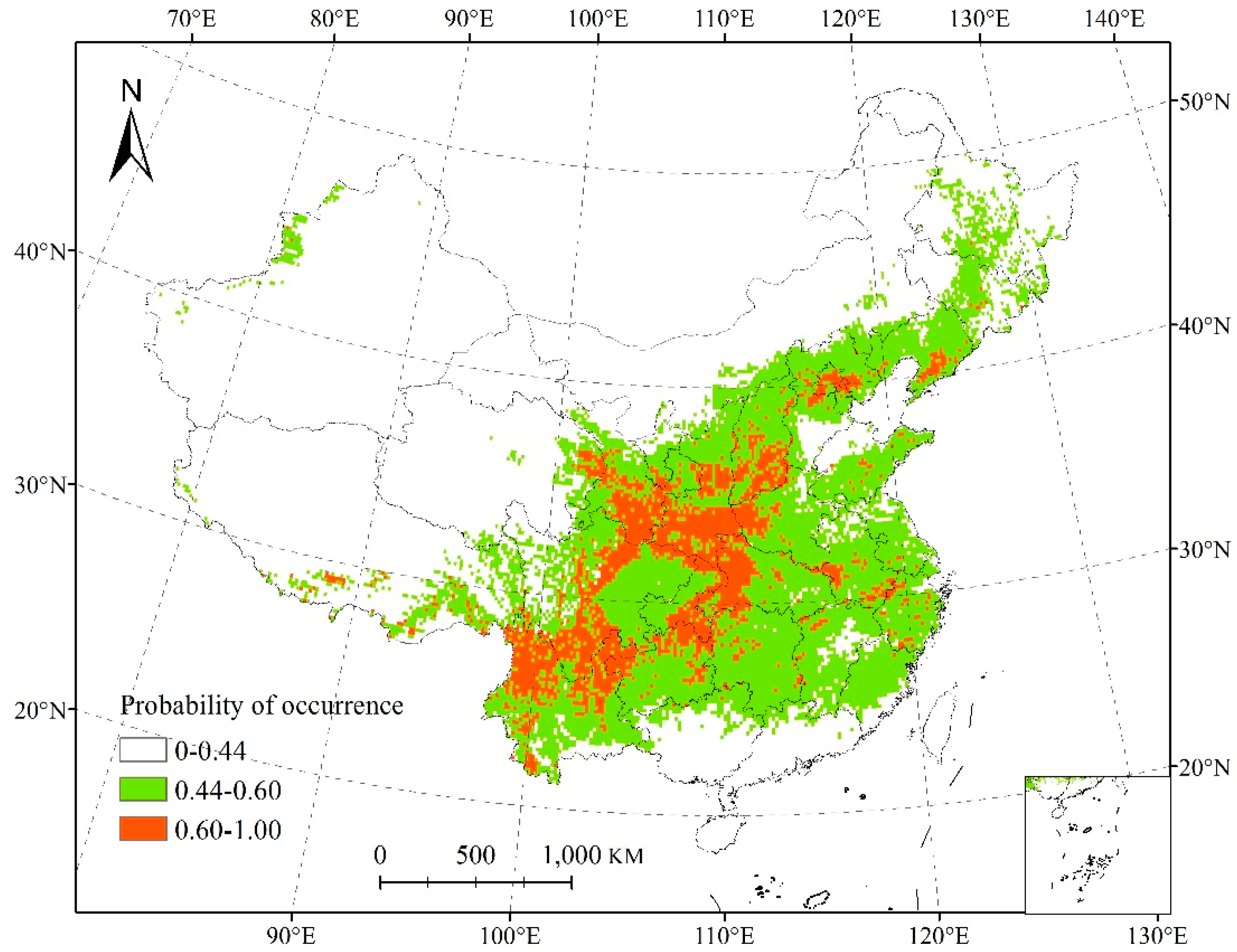
3.1. Species Distribution Model and Its Accuracy

China was divided into 26,137 grid cells, with 2673 of them (10.22%) having exact geographic coordinates. Models for the Salicaceae family with a cross-validation AUC close to 0.75 were considered useful in our study. The training and testing of the AUC value for the 215 species models was >0.8, which indicated these models were non-random and could be reliably used for modeling the relationship between diversity patterns and environmental factors. Potential suitable habitat areas are currently widely distributed in China’s subtropical and warm temperate zones, but occurred mainly in its central and southwestern regions. Highly suitable areas were found in the Hengduan Mountains, Daba Mountains, and Qinling Mountains (Figure 1).

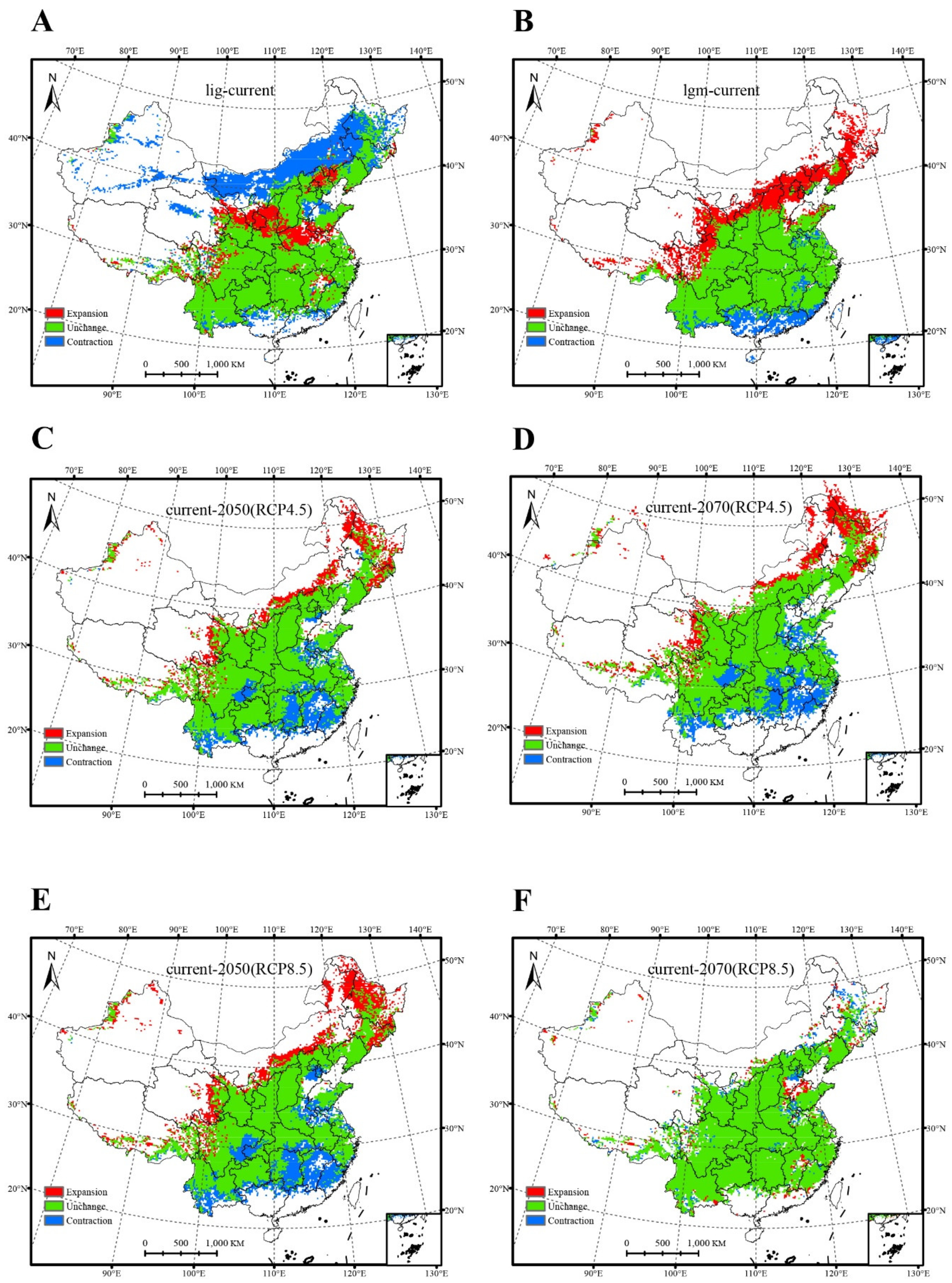
3.2. Changes in the Potential Range of Salicaceae

Compared with the LIG, the niche model predicted losses in current suitable habitat areas mainly distributed in the middle temperate zone of northern China, namely Inner Mongolia, Heilongjiang, Jilin, Xinjiang, Qinghai, and Gansu (Figure 2A). The projected area of reduction amounted to 139.72 × 10⁴ km2, which accounts for 38.67% of the currently suitable area (Table 2). This range contraction was mainly concentrated in high latitude areas. Conversely, the gains in suitable range area totaled 62.79 × 10⁴ km2 (17.38% of the currently suitable area), mostly distributed in provinces of Ningxia, Shaanxi, Gansu, Henan, and Hebei. Expansion occurred mainly in the mid-latitudes. Overall, from the last glacial period to the present, we saw a wide range of contractions, with the total suitable habitats reduced by ca. 76.92 × 10⁴ km2 (Figure 2A, Table 2). In contrast to the LIG, the suitable habitats increased significantly—the total suitable habitat area increased by ca. 69.63 × 10⁴ km2—from the LGM to the present (Figure 2B, Table 2). These gains amounted to 106.88 × 10⁴ km2, or 29.58% of the currently suitable area, and were concentrated in parts of Tibet, Sichuan, Qinghai, Gansu, Ningxia, Inner Mongolia, Shannxi, Hebei, Liaoning, Beijing, Tianjin, Jilin, and Heilongjiang. Expansion in habitats increased with increasing latitude. The predicted losses occurred mainly in the subtropics of southern China, namely Guangxi, Guangdong, and Fujian, covering an area of ca. 37.25 × 10⁴ km2 (10.31% of the currently suitable area; Figure 2B, Table 2).
Under all four future climate scenario/year combinations of RCP4.5-2050, RCP4.5-2070, RCP8.5-2050, and RCP8.5-2070, the predicted area of suitable habitats shrunk (Table 2). The parts of Salicaceae’s range with high risks of habitat loss were distributed in subtropical zones, including southern and eastern regions of China, Jiangxi, Fujian, eastern Hunan, southwestern Yunnan, northern Guangxi and Guangdong, southeast Hubei, the border of Chongqing and Sichuan, the junction of Anhui, Henan, Jiangsu, and Shandong, as well in limited regions of Hebei, Tianjin, and Beijing (Figure 2C–F). The Maxent model predicted total losses of 20.21 × 10⁴ km2~82.06 × 10⁴ km2 (5.59%~22.71% of the currently suitable area; Table 2). These losses were mostly concentrated at low elevation and the contraction generally increased at lower latitudes. Most of the predicted gains in suitable habitat area were restricted to Salicaceae’s range in the north of China’s warm temperate zone (Tibet, Sichuan, Qinghai, Inner Mongolia, Heilongjiang, and Jilin), which amounted to ca. 20.18 × 10⁴ km2~78.06 × 10⁴ km2 (5.58%~21.60% of the currently suitable area; Table 2), all located in high latitude regions. The total potential suitable habitat area decreased under the four future climatic scenario/years, with contractions in Jiangxi, Fujian, and eastern Hunan most apparent (Figure 2C–F).

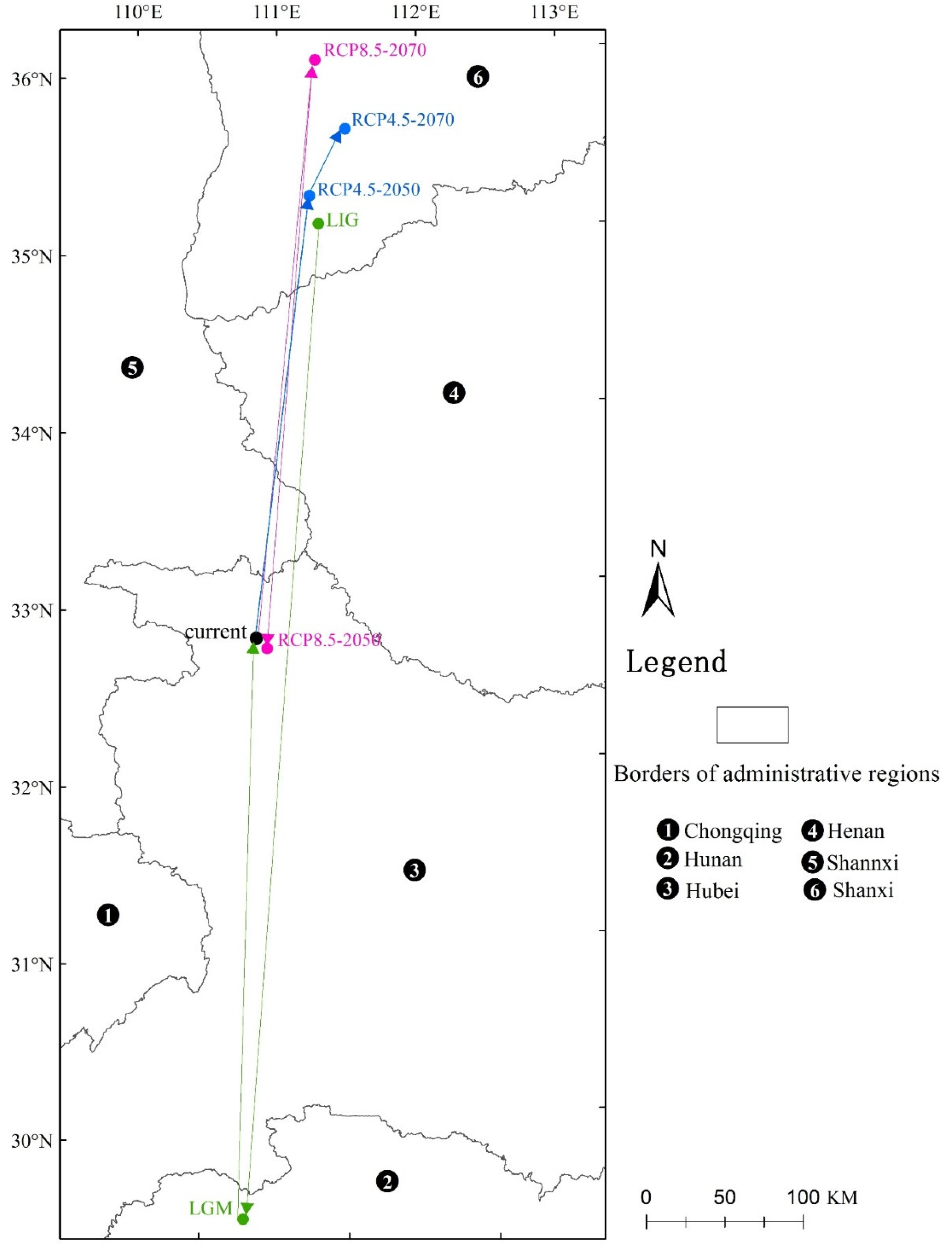
3.3. Core Distributional Shifts

The center of predicted suitable areas in the present was located in the Hubei province, with geographical coordinates of 110.62 E and 32.79 N (Figure 3). The centroid of potential suitable habitats in the LIG shifted to northern regions (111.11 E, 35.12 N) and high latitudes. By contrast, the centroid in the LGM period shifted to southern regions and low latitude (110.28 E, 29.52 N). Under the future climate scenario/years combinations, the center of potential suitable habitats was located at more northerly areas with higher latitudes, except under RCP8.5-2070. Evidently, the distribution center of Salicaceae plants is likely to shift to high latitudes from the LGM into the future (Figure 3).

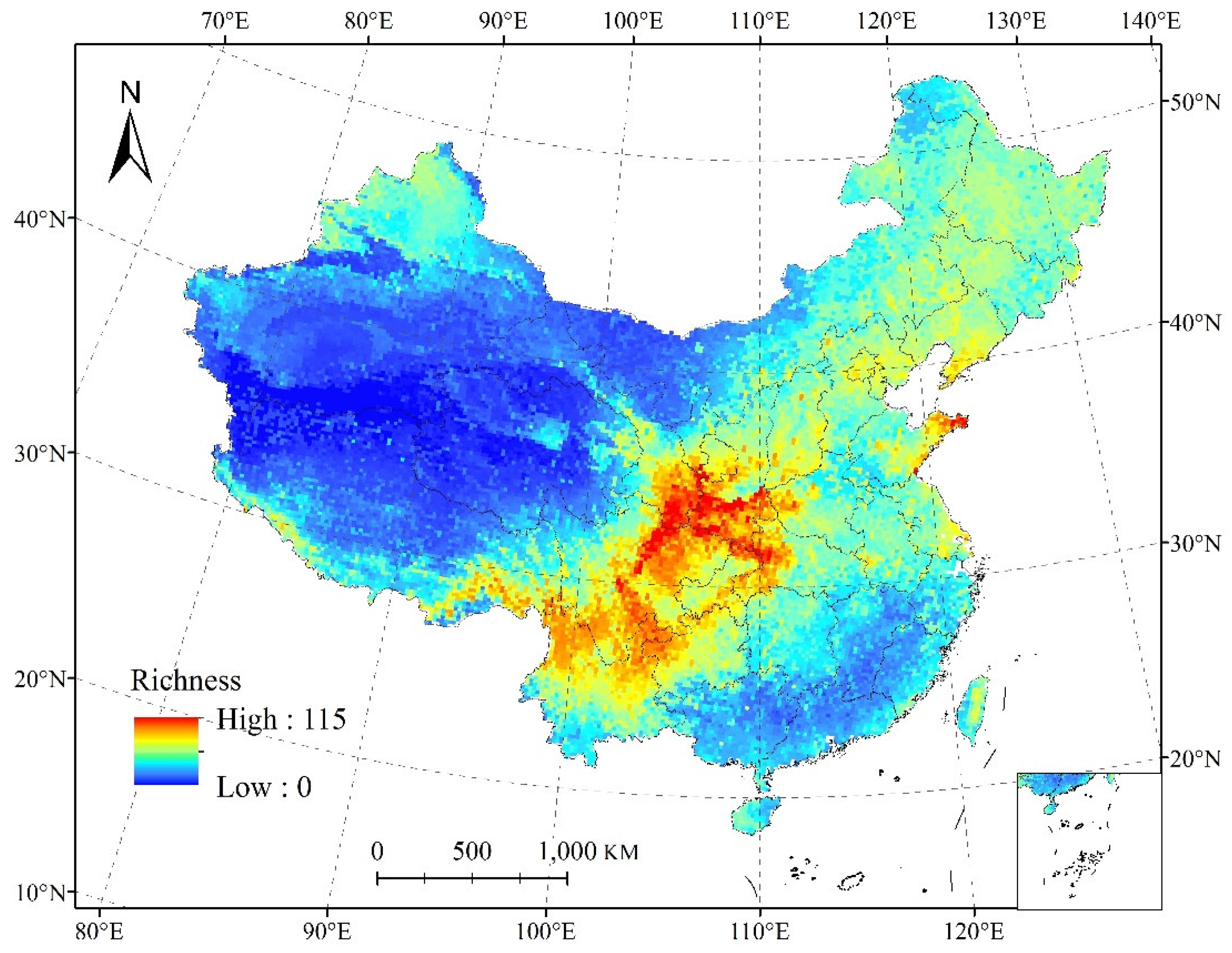
3.4. Relationships between Species Richness and Environmental Parameters

The pattern of Salicaceae species richness was obtained from 215 species potential distribution model layers. Botanical species richness ranged from 0 to 115 in each grid cell in China, with an average of 35 per cell. The southwest and central regions of China showed the highest Salicaceae species diversity, which included the eastern Tibet Plateau and the Hengduan Mountains, Qinling Mountains, Daba Mountains, Dalou Mountains, Wumeng Mountains, Wulian Mountains, Longmen Mountains, Daxue Mountains, Liupan Mountains, and Kunji Mountains. In short, high species diversity was mainly concentrated in alpine areas. The northeast region of China ranked second in species diversity. By contrast, species diversity of northwest China, south China, and the western Tibet Plateau were relatively low (Figure 4).
The GLMs showed that the variables related to contemporary energy had stronger explanatory ability than contemporary water availability, soil conditions, heterogeneity, and historical climate change. Specifically, UV-B radiation was the strongest variable, as it explained 35% (p < 0.05). Species richness decreased as UV-B factors and annual mean temperature increased, indicating that areas with high species diversity are warm with low UV-B radiation. Elevation and anomaly of precipitation seasonality both adversely affected species diversity patterning, while annual precipitation and nitrogen content of the topsoil were positively associated with it. Those places featuring a climate warmer and wetter than in the LGM tended to have more Salicaceae species than other regions (Table 3).

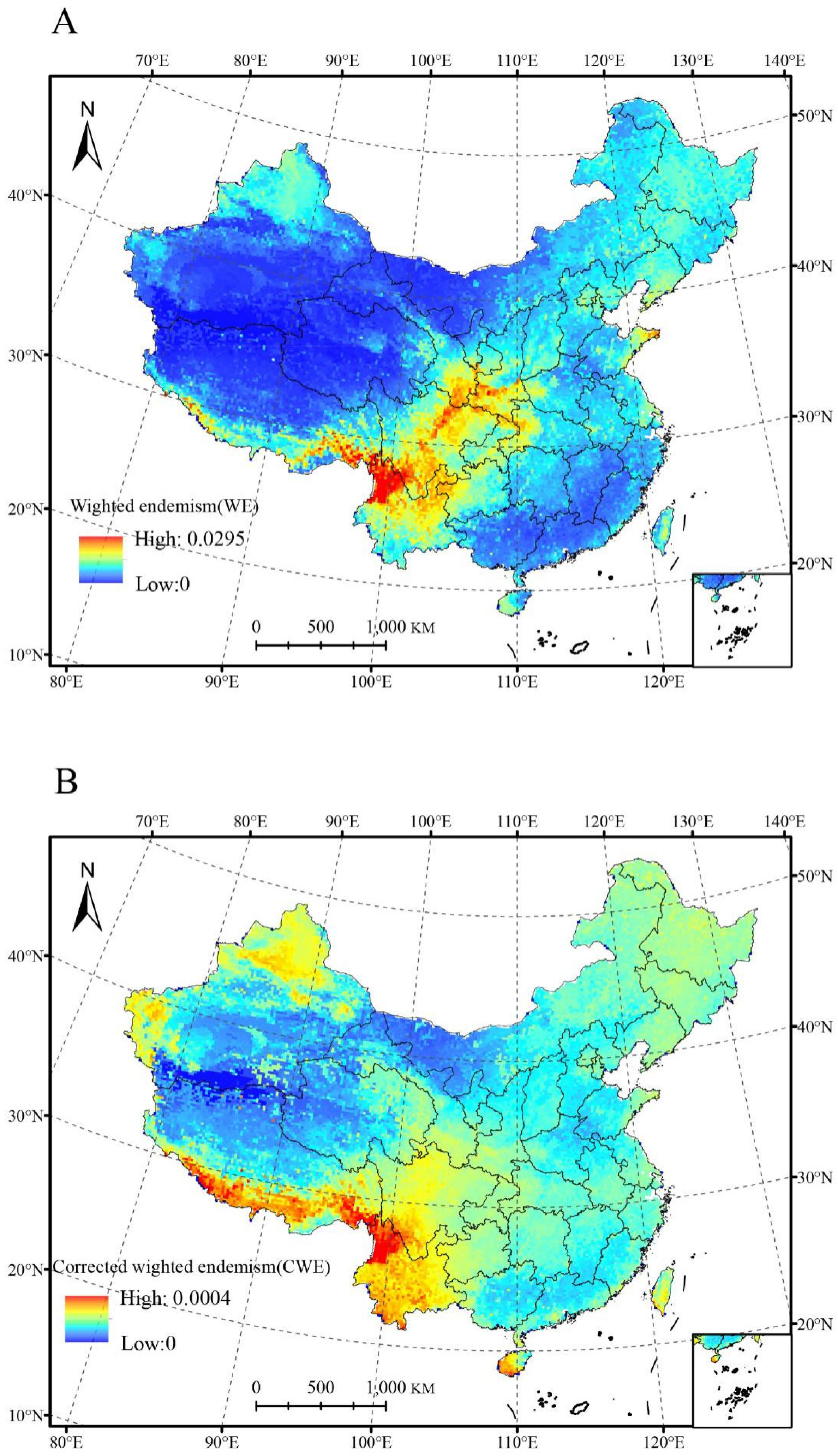
3.5. Relationships between Weighted Endemism (WE), Corrected-Weighted Endemism (CWE), and Environmental Factors

Plant-weighted endemism ranged from 0 to 0.0295 in each grid cell in China, with an average value of 0.0068, and 1.61% of the total grids had more values >0.0200 (Figure 5A). Weighted-endemism followed a similar pattern as did that found for species richness. The Himalayas, and the mountains of Hengduan, Qinling, Daba, Longmen, Wumeng, Wulian, Yunling, and Kunji all featured high values of weighted endemism. The corrected-weighted endemism ranged from 0 to 0.0004 (Figure 5B), with the high values concentrated in northwest China, including the Himalayas and Hengduan Mountains. The latter is where endemic species of Salicaceae had their ranges most narrowly distributed.
The GLMs showed that both historical climate change and contemporary water availability were the main factors shaping the patterns of weighted endemism (Table 3). The anomalies of precipitation seasonality and annual precipitation explained 22% of its variation. While nitrogen content of topsoil and UV-B radiation also had significant positive effects on the corrected-weighted endemism pattern. Elevation was a significant factor in the three types of pattern, but it showed weaker explanatory power for the weighted endemism and corrected-weighted endemism patterns. The relationships between nitrogen content of topsoil and patterns of weighted endemism and corrected-weighted endemism were significant, showing strong positive correlations (Table 3).

4. Discussion

4.1. Changes in the Potential Range of Salicaceae in China

Using the georeferenced occurrence data of Salicaceae, our results showed that its predicted potential distribution area covers most regions of China. The predicted results are consistent with the actual distribution of Salicaceae plants in China, which features strong regularity and forms part of the temperate deciduous forest community. The similarity of all the plant species—they are deciduous, water demanding, and require a temperate bioclimate, to name a few key traits—and the model’s effective prediction accuracy (>0.7) support the generalization of our results. Second, by simulating Salicaceae species’ ranges and patterns in different periods we could infer their historical and future population dynamics (Figure S1). Salicaceae may have experienced a significant and extensive expansion from south to north during the Last Inter Glacial period (LIG). This strongly suggests Salicaceae can track suitable niches during the glacial and interglacial cycles, in that its distribution shifted southward in the glacial period but shifted back northward after the glacial period. Salicaceae is a group of plants whose ecological amplitude is large and they can adapt to many different ecological environments, from those ranging from high (~20 °C) to low (~3 °C) temperatures, and from swamp to sand habitats [66,67]. The temperature (average: ~5 °C) and rainfall (average: ~557 mm) in the LIG were within the tolerance levels of Salicaceae species. However, with significant reductions in temperature and rainfall, the climate became drier and colder in the Last Glacial Maximum (LGM) [68,69]. In response, because those areas with suitable habitat were generally greatly reduced, Salicaceae’s distribution range retreated to areas low in elevation [70]. Therefore, from these results we infer this plant family was able to spread rapidly in the glacial-interglacial cycle [11]. Most of its species (i.e., members of Salix subgenera Chamaetia and Vetrix, represent ca. 75% species of Salicaceae) are Arctic-alpine taxa well adapted to cold and hostile environments [71]. Therefore, the considerable northward expansion in China of the Salicaceae distribution area is both plausible and reasonable. In sum, Quaternary climate change profoundly influenced the historical spatial population dynamics of ancient Chinese Salicaceae species [72].
As the climate warms, extreme weather events are becoming more frequent and intense [73,74,75]. Climate research has made much progress in recent years, but most of it is based on qualitative rather than quantitative analyses [76,77,78,79]. In our study, we conducted a detailed quantitative analysis of the potential distribution of Salicaceae in the future. Nevertheless, simulation results are expected to vary between different climate models [80,81]. Salicaceae are widely distributed, occurring in Africa, Europe, Asia, South America, and North America from ca. 82° N to 52° S [82], but their habitats are often fragmented. East Asia is the present distribution center of modern species of Salicaceae, and China harbors the most species numerically.
Our modeling study predicted ca. 361.33 × 10⁴ km2 for Salicaceae species under the present climate scenario with its core distributional area being Hubei Province, which is broadly within the distribution area of extant Salicaceae. In our study’s projections, the centroid of suitable distribution shifted northerly to higher latitude areas under the future climate scenarios, and this trend agrees with other works [83,84,85,86]. Our results also show that if global warming becomes more intense, the suitable range of Salicaceae faces the risk of reduction under the medium and high carbon dioxide emission scenarios (RCP4.5 and RCP8.5), a result that is also in line with previous studies [79,87]. Species of Salicaceae are, therefore, clearly vulnerable to climate change effects, with its range contractions mainly concentrated at low latitudes [88,89,90]. Nevertheless, since the model involved all species of the family these results are not applicable to endangered species or any other particular species. Earlier studies by Bomhard et al. [91] and Midgley et al. [92] suggested that future climate change and land-use transformations would have synergistic effects on species habitats, giving rise to unsuitable habitats for their persistence. In this context, we found that Salicaceae species do display strong adaptability under the present and future climate scenarios; however, some of the suitable range may become unsuitable due to intense disturbance by human activities and land-use changes. For example, much of the suitable range for Salicaceae plants in China has been converted into farmland or construction land [93]. Clearly, the effects from future land-use changes should also be taken into account in species distribution models [94]. We suggest that local protection measures (Figure S3) can be adopted to reduce anthropocentric-driven damage to suitable habitat. Meanwhile, we can also try to implement ex situ protection projects, such as transplanting species from a threatened area to a site with non- or less-degraded habitat, or by planting them in multiple botanical gardens.

4.2. Species Richness and Endemism Patterns of Salicaceae in China

Using the distributions of 215 Salicaceae species, we explored their large-scale variation in species richness and endemism and the environment variables likely determining these patterns. China is famous for its high species diversity; better documenting and understanding of its diversity and endemic patterns will inform and strengthen biological conservation, by providing baselines for biodiversity management and relevant policy-making. China’s southwest, lying south of the Hengduan Mountains, is well known for its high suitability for and diversity of Salicaceae species (Figure 2, Figure 4 and Figure 5). Our variance partition analyses revealed pure effects of contemporary environments and historical climate change that respectively accounted for 47.90% and 18.10% of the variance in Salicaceae diversity patterns across China (Figure S2). Consistent with other research [14,95], our study showed the climate exerts a important influence on Salicaceae species richness, weighted endemism, and corrected-weighted endemism (Table 3 and Figure 2 and Figure S2). For all three, the most important factor was the contemporary environment (energy, water availability and soil conditions), since it had the strongest explanatory power (Table 3). This indicates high species diversity of Salicaceae mostly occurs in areas with relatively warm and high humidity [96]. High temperatures at low latitudes may curtail breeding times and accelerate species formation, favoring the emergence of new plant species [97]. This is consistent with evidence that imposed warming considerably increased the root, stem, and leaf biomass of Salicaceae plants [98] with drought strongly impeding their growth [99,100]. Meanwhile, considering that Salicaceae species originated in the temperate zone [101] and most of them prefer wet environments [102], the positive association between precipitation, temperature and species diversity lends supports to the water–energy dynamic equilibrium hypothesis as a species richness formation mechanism. It has been shown that water–energy dynamics (precipitation and coldest monthly evapotranspiration) were the main factors affecting the diversity of South African trees [103,104,105]. Other studies have found biodiversity patterns that were also related to water availability [106,107]. Temperature and liquid water are not only vital for plants to absorb and transport nutrients but also mediate key physiological activities (e.g., photosynthesis) [108,109].
Besides water and temperature, our results suggested UV-B radiation also contributes to the biodiversity pattern of Salicaceae plants. The negative associations indicate that where UV-B radiation is intense, both species richness and endemism are lower. UV-B radiation is a factor known to limit the distribution range of terrestrial and marine life: its negative relationship with biodiversity patterns arises from its adverse effects on the protective mechanisms and organs of plants [110]. Related research has also found that high-intensity UV-B radiation can reduce the photosynthetic performance of Salicaceae species [43,111,112], in addition to diminishing the biomass accumulation [16], seed germination [113] and membrane structure integrity [44] of plants. Therefore, we propose that, generally, intensive UV-B radiation reduces Salicaceae plant biodiversity. Compared with other environmental variables, the association between soil fertility and biodiversity pattern was relatively weak, which is in line with other research [114]. Nevertheless, it worth emphasizing that topsoil nitrogen content makes a non-trivial contribution to the diversity patterns of Salicaceae species. This may be linked to how N can markedly influence gender differences and competitiveness between the two sexes in these plants [47]. Some studies do show that temperature stability [115] and historical climatic stability [116] also affect species diversity patterns. We found historical geological processes also played an essential role by altering the range (Figure 2A,B), diversity and endemism (Table 3, Figure S2) of Salicaceae species during the glacial period. Thus, while contemporary water-energy and historical climate change both have significant impacts on Salicaceae, other factors (such as disturbance history) warrant quantitative study in future research [117]. It is well known that the ozone layer protects the forests and other life forms on the Earth’s surface from the sun’s harmful ultraviolet radiation [118]. During the last few decades, the stratospheric ozone layer has been depleted by anthropogenic pollutants such as chlorofluorocarbons (CFCS), leading to an increase in surface-level ultraviolet radiation. As a result of the 1987 Montreal protocol and its amendments, the anthropogenic loading of ozone-depleting substances in the atmosphere is being reduced. Nevertheless, future climate change could cause extreme dynamic events [119], volcanic eruptions [120] and irregular changes in solar flux [121], all of which are likely to damage the ozone layer. Caldwell’s results showed that for every 1% reduction in ozone, the surface’s UV-B (280–320 mm) radiation increases by 2% [122]. With greater UV-B radiation possible in the future, the geographical distribution and species diversity of Salicaceae plants may become threatened.

5. Conclusions

Based on niche model, we propose the Salicaceae family underwent an extensive population expansion of its species during the LIG, but retreated to low latitudes during the LGM. As climate warming intensifies, suitable habitats will shift to higher latitudes while those at lower latitudes will contract in area and abundance. Habitats of Salicaceae in China are most likely to be lost in the future, especially in Jiangxi, Fujian, and eastern Hunan. The western and central regions of China currently show the highest diversity of Salicaceae species. Because they are typical pioneer plants, with a strong ability to disperse and colonize, they could fill new or open habitats easily; these traits make it difficult to resort to a single hypothesis to reveal their pattern of species diversity. Nevertheless, our results point to the water–energy dynamic equilibrium and historical geological processes as being key drivers of Salicaceae diversity patterns in China. Our study could thus assist in the conservation and sustainable use of Salicaceae, and our results provide a solid baseline for biodiversity management and relevant policy-making for these important woody plants.

Supplementary Materials

The following are available online at https://www.mdpi.com/1999-4907/10/3/220/s1, Table S1: The filtered occurrence data of Salicaceae; Table S2: The 215 species catalogue used to construct the species diversity pattern of Salicaceae; Table S3: Spearman’s rank correlation coefficients (rs) for the 5 bioclimatic variables and elevation. Bio1: Annual mean temperature, Bio3: Isothermality (Bio2/Bio7) (*100), Bio7: Temperature annual range (Bio5-Bio6), Bio12: Annual precipitation, Bio15: Precipitation seasonality (coefficient of variation); Table: S4 Spearman’s rank correlation coefficients (rs) for the 5 soil variables. S-CE: Cation exchange capacity (CEC) clay subsoil, T-BS: Base saturation% topsoil, T-C: Organic carbon pool topsoil, T-N: Nitrogen % topsoil, Drain: Soil drainage class; Figure S1: The potential distribution pattern of Salicaceae plants in China under different combination of climate scenario/years, using the Albers projection. (A) the potential distribution pattern under the Last Inter Glacial; (B) the potential distribution pattern under the Last Glacial Maximum; (C) the potential distribution pattern under future climate scenario RCP4.5 in 2050; (D) the potential distribution pattern under future climate scenario RCP4.5 in 2070; (E) the potential distribution pattern under future climate scenario RCP8.5 in 2050; (F) the potential distribution pattern under future climate scenario RCP8.5 in 2070; Figure S2: The pure and combined effect of contemporary environments and historical climate changes in shaping Salix species diversity; Figure S3: The spatial pattern of nature reserves and the shrinking distribution range under the future climate scenarios.

Author Contributions

Conceptualization, W.L., M.S., Y.H., H.S. and J.C.; Data curation, W.L., M.S. and K.C.; Formal analysis, W.L., Y.H., H.S. and J.C.; Funding acquisition, H.S. and J.C.; Investigation, W.L., Y.H. and K.C.; Methodology, W.L., M.S. and K.C.; Project administration, W.L., H.S. and J.C.; Resources, W.L., M.S., Y.H. and J.C.; Software, W.L., M.S. and Y.H.; Supervision, Y.H., H.S. and J.C.; Validation, W.L., M.S., K.C. and H.S.; Visualization, W.L. and K.C.; Writing—original draft, W.L. and J.C.; Writing—review and editing, W.L., H.S. and J.C.

Funding

This study was supported by grants from the National Natural Science Foundation of China (NSFC 31590823 to HS, 31670198 to JC, 31560062 to YH); the Science and Technology Research Program of Kunming Institute of Botany, the Chinese Academy of Sciences, Grant NO. KIB2016005; and the Youth Innovation Promotion Association, the Chinese Academy of Sciences.

Conflicts of Interest

The authors declare that they have no competing interests.

References

  1. Hong, Q.; Ricklefs, R.E. Large–scale processes and the asian bias in species diversity of temperate plants. Nature 2000, 407, 180–182. [Google Scholar]
  2. Buckley, L.B.; Davies, T.J.; Ackerly, D.D.; Kraft, N.J.; Harrison, S.P.; Anacker, B.L.; Cornell, H.V.; Damschen, E.I.; Grytnes, J.A.; Hawkins, B.A.; et al. Phylogeny, niche conservatism and the latitudinal diversity gradient in mammals. Proc. R. Soc. 2010, 277, 2131–2138. [Google Scholar] [CrossRef] [PubMed]
  3. Brown, J.H. Why are there so many species in the tropics? J. Biogeogr. 2014, 41, 8–22. [Google Scholar] [CrossRef] [PubMed]
  4. Beck, J.; Ballesteros-Mejia, L.; Buchmann, C.M.; Dengler, J.; Fritz, S.A.; Gruber, B.; Hof, C.; Jansen, F.; Knapp, S.; Kreft, H.; et al. What’s on the horizon for macroecology? Ecography 2012, 35, 673–683. [Google Scholar] [CrossRef]
  5. Hawkins, B.A. Invited views in basic and applied ecology: Are we making progress toward understanding the global diversity gradient? Basic Appl. Ecol. 2004, 5, 1–3. [Google Scholar] [CrossRef]
  6. Brown, J.H.; Gillooly, J.F.; Allen, A.P.; Savage, V.M.; West, G.B. Toward a metabolic theory of ecology. Ecology 2004, 85, 1771–1789. [Google Scholar] [CrossRef]
  7. Colwell, R.K.; Rahbek, C.; Gotelli, N.J. The mid-domain effect and species richness patterns: What have we learned so far? Am. Nat. 2004, 163, E1–E23. [Google Scholar] [CrossRef] [PubMed]
  8. Joy, J.B. The global diversity of birds in space and time. Nature 2012, 491, 444–448. [Google Scholar]
  9. Jansson, R. Global variation in diversification rates of flowering plants: Energy vs. Climate change. Ecol. Lett. 2008, 11, 173–183. [Google Scholar] [CrossRef] [PubMed]
  10. Mittelbach, G.G.; Schemske, D.W.; Cornell, H.V.; Allen, A.P.; Brown, J.M.; Bush, M.B.; Harrison, S.P.; Hurlbert, A.H.; Knowlton, N.; Lessios, H.A.; et al. Evolution and the latitudinal diversity gradient: Speciation, extinction and biogeography. Ecol. Lett. 2007, 10, 315–331. [Google Scholar] [CrossRef] [PubMed]
  11. Levsen, N.; Tiffin, P.; Olson, M. Pleistocene speciation in the genus populus (salicaceae). Syst. Biol. 2012, 61, 401–412. [Google Scholar] [CrossRef] [PubMed]
  12. Lee, C.B.; Chun, J.H. Retracted article: Habitat heterogeneity and climate explain plant diversity patterns along an extensive environmental gradient in the temperate forests of south korea. Folia Geobot. 2016, 1. [Google Scholar] [CrossRef]
  13. Veloz, S.D.; Williams, J.W.; Blois, J.L.; He, F.; Otto-Bliesner, B.; Liu, Z. No–analog climates and shifting realized niches during the late quaternary: Implications for 21st–century predictions by species distribution models. Glob. Chang. Biol. 2012, 18, 1698–1713. [Google Scholar] [CrossRef]
  14. Currie, D.J. Energy and large-scale patterns of animal and plant–species richness. Am. Nat. 1991, 137, 27–49. [Google Scholar] [CrossRef]
  15. Latham, R.E.; Ricklefs, R.E. Global patterns of tree species richness in moist forests: Energy-diversity theory does not account for variation in species richness. Oikos 1993, 67, 325–333. [Google Scholar] [CrossRef]
  16. Xu, X.; Zhao, H.; Zhang, X.; Hänninen, H.; Korpelainen, H.; Li, C. Different growth sensitivity to enhanced uv-b radiation between male and female populus cathayana. Tree Physiol. 2010, 30, 1489–1498. [Google Scholar] [CrossRef] [PubMed]
  17. Clarke, A.; Gaston, K.J. Climate, energy and diversity. Proc. R. Soc. 2006, 273, 2257–2266. [Google Scholar] [CrossRef] [PubMed]
  18. Qin, H.; Dong, G.; Zhang, Y.; Zhang, F.; Wang, M. Patterns of species and phylogenetic diversity of pinus tabuliformis forests in the eastern loess plateau, china. For. Ecol. Manag. 2017, 394, 42–51. [Google Scholar] [CrossRef]
  19. Thuiller, W.; Lavergne, S.; Roquet, C.; Boulangeat, I.; Lafourcade, B.; Araujo, M.B. Consequences of climate change on the tree of life in europe. Nature 2011, 470, 531–534. [Google Scholar] [CrossRef] [PubMed]
  20. Pio, D.V.; Engler, R.; Linder, H.P.; Monadjem, A.; Cotterill, F.P.D.; Taylor, P.J.; Schoeman, M.C.; Price, B.W.; Villet, M.H.; Eick, G.; et al. Climate change effects on animal and plant phylogenetic diversity in southern africa. Glob. Chang. Biol. 2014, 20, 1538–1549. [Google Scholar] [CrossRef]
  21. Hultine, K.R.; Burtch, K.G.; Ehleringer, J.R. Gender specific patterns of carbon uptake and water use in a dominant riparian tree species exposed to a warming climate. Glob. Chang. Biol. 2013, 19, 3390–3405. [Google Scholar] [CrossRef] [PubMed]
  22. González-Orozco, C.E.; Pollock, L.J.; Thornhill, A.H.; Mishler, B.D.; Knerr, N.; Laffan, S.W.; Miller, J.T.; Rosauer, D.F.; Faith, D.P.; Nipperess, D.A.; et al. Phylogenetic approaches reveal biodiversity threats under climate change. Nat. Clim. Chang. 2016, 6, 1110–1114. [Google Scholar] [CrossRef]
  23. Bellard, C.; Bertelsmeier, C.; Leadley, P.; Thuiller, W.; Courchamp, F. Impacts of climate change on the future of biodiversity. Ecol. Lett. 2012, 15, 365–377. [Google Scholar] [CrossRef] [PubMed]
  24. Stocker, T.F.; Qin, D.; Plattner, G.K.; Tignor, M.; Allen, S.K.; Boschung, J.; Nauels, A.; Xia, Y.; Bex, B.; Midgley, B.M. IPCC, 2013: Climate change 2013: The physical science basis. Contribution of working group i to the fifth assessment report of the intergovernmental panel on climate change. Comput. Geom. 2013, 18, 95–123. [Google Scholar]
  25. Parmesan, C. Ecological and evolutionary responses to recent climate change. Annu. Rev. Ecol. Evol. Syst. 2006, 37, 637–669. [Google Scholar] [CrossRef]
  26. Myers-Smith, I.H.; Forbes, B.C.; Wilmking, M.; Hallinger, M.; Lantz, T.; Blok, D.; Tape, K.D.; Macias-Fauria, M.; Sass-Klaassen, U.; Lévesque, E.; et al. Shrub expansion in tundra ecosystems: Dynamics, impacts and research priorities. Environ. Res. Lett. 2011, 6, 045509. [Google Scholar] [CrossRef]
  27. Jones, M.H. Sex- and habitat-specific responses of a high arctic willow, salix arctica, to experimental climate change. Oikos 1999, 87, 129–138. [Google Scholar] [CrossRef]
  28. Fang, Z.F.; Zhao, S.D.; Skvortsov, A.K. Salicaceae. Flora China 1999, 4, 139–274. [Google Scholar]
  29. Zhao, S.D. Distribution of willows (salix) in china. Acta Phytotaxon. Sin. 1987, 25, 114–124. [Google Scholar]
  30. Karp, A.; Shield, I. Bioenergy from plants and the sustainable yield challenge. New Phytol. 2008, 179, 15–32. [Google Scholar] [CrossRef] [PubMed]
  31. Chen, J.H.; Sun, H.; Wen, J.; Yang, Y.P. Molecular phylogeny of salix l. (salicaceae) inferred from three chloroplast datasets and its systematic implications. Taxon 2010, 59, 29–37. [Google Scholar] [CrossRef]
  32. Wang, Q.; Su, X.; Shrestha, N.; Liu, Y.; Wang, S.; Xu, X.; Wang, Z. Historical factors shaped species diversity and composition of salix in eastern asia. Sci. Rep. 2017, 7, 42038. [Google Scholar] [CrossRef] [PubMed]
  33. Warren, D.L. In defense of ‘niche modeling’. Trends Ecol. Evol. 2012, 27, 497–500. [Google Scholar] [CrossRef] [PubMed]
  34. Peterson, A.T.; Soberón, J.; Pearson, R.G.; Anderson, R.P.; Martínez-Meyer, E.; Nakamura, M.; Araújo, M.B. Ecological niches and geographic distribution. Monogr. Popul. Biol. 2011, 49, 328. [Google Scholar]
  35. Chen, F.T. Phylogeography of Rehmannia (Scrophulariaceae); Northwest University: Xi’an, China, 2015. [Google Scholar]
  36. Wang, Q.; Wei, Y.K.; Huang, Y.B. Research on distribution pattern of subg. Salvia benth. (lamiaceae), an important group of medicinal plants in east asia. Acta Ecol. Sin. 2015, 5, 470–479. [Google Scholar]
  37. Beck, J.; Böller, M.; Erhardt, A.; Schwanghart, W. Spatial bias in the gbif database and its effect on modeling species’ geographic distributions. Ecol. Inform. 2014, 19, 10–15. [Google Scholar] [CrossRef]
  38. Fourcade, Y.; Engler, J.O.; Rödder, D.; Secondi, J. Mapping species distributions with maxent using a geographically biased sample of presence data: A performance assessment of methods for correcting sampling bias. PLoS ONE 2014, 9, e97122. [Google Scholar] [CrossRef] [PubMed]
  39. Zhang, M.G.; Slik, J.W.; Ma, K.P. Using species distribution modeling to delineate the botanical richness patterns and phytogeographical regions of china. Sci. Rep. 2016, 6, 22400. [Google Scholar] [CrossRef] [PubMed]
  40. Pearson, R.G.; Raxworthy, C.J.; Nakamura, M.; Townsend Peterson, A. Original article: Predicting species distributions from small numbers of occurrence records: A test case using cryptic geckos in madagascar. J. Biogeogr. 2007, 34, 102–117. [Google Scholar] [CrossRef]
  41. Stevens, G.C. The latitudinal gradient in geographical range: How so many species coexist in the tropics. Am. Nat. 1989, 133, 240–256. [Google Scholar] [CrossRef]
  42. Yan, Y.; Yang, X.; Tang, Z. Patterns of species diversity and phylogenetic structure of vascular plants on the qinghai-tibetan plateau. Ecol. Evol. 2013, 3, 4584–4595. [Google Scholar] [CrossRef] [PubMed]
  43. Nybakken, L.; Hörkkä, R.; Julkunen-Tiitto, R. Combined enhancements of temperature and uvb influence growth and phenolics in clones of the sexually dimorphic salix myrsinifolia. Physiol. Plant. 2012, 145, 551–564. [Google Scholar] [CrossRef] [PubMed]
  44. Randriamanana, T.R.; Nissinen, K.; Moilanen, J.; Nybakken, L.; Julkunen-Tiitto, R. Long-term uv-b and temperature enhancements suggest that females of salix myrsinifolia plants are more tolerant to uv-b than males. Environ. Exp. Bot. 2015, 109, 296–305. [Google Scholar] [CrossRef]
  45. Feng, L.; Hao, J.; Zhang, Y.; Sheng, Z. Sexual differences in defensive and protective mechanisms of populus cathayana exposed to high uv-b radiation and low soil nutrient status. Physiol. Plant. 2014, 151, 434–445. [Google Scholar] [CrossRef]
  46. Hageer, Y.; Esperónrodríguez, M.; Baumgartner, J.B.; Beaumont, L.J. Climate, soil or both? Which variables are better predictors of the distributions of australian shrub species? PeerJ 2017, 5, e3446. [Google Scholar] [CrossRef] [PubMed]
  47. Chen, J.; Dong, T.; Duan, B.; Korpelainen, H.; Niinemets, Ü.; Li, C. Sexual competition and n supply interactively affect the dimorphism and competiveness of opposite sexes in populus cathayana. Plant Cell Environ. 2015, 38, 1285–1298. [Google Scholar] [CrossRef] [PubMed]
  48. Moor, H.; Hylander, K.; Norberg, J. Predicting climate change effects on wetland ecosystem services using species distribution modeling and plant functional traits. Ambio 2015, 44 (Suppl. 1), S113–S126. [Google Scholar] [CrossRef]
  49. Fitzpatrick, M.C.; Gotelli, N.J.; Ellison, A.M. Maxent versus maxlike: Empirical comparisons with ant species distributions. Ecosphere 2013, 4, art55. [Google Scholar] [CrossRef]
  50. Guisan, A.; Thuiller, W. Predicting species distribution: Offering more than simple habitat models. Ecol. Lett. 2005, 8, 993–1009. [Google Scholar] [CrossRef]
  51. Phillips, S.J.; Anderson, R.P.; Schapire, R.E. Maximum entropy modeling of species geographic distributions. Ecol. Model. 2006, 190, 231–259. [Google Scholar] [CrossRef]
  52. Bertrand, R.; Perez, V.; Gégout, J.C. Disregarding the edaphic dimension in species distribution models leads to the omission of crucial spatial information under climate change: The case of quercus pubescensin france. Glob. Chang. Biol. 2012, 18, 2648–2660. [Google Scholar] [CrossRef]
  53. Araújo, M.B.; Peterson, A.T. Uses and misuses of bioclimatic envelope modeling. Ecology 2012, 93, 1527–1539. [Google Scholar] [CrossRef] [PubMed]
  54. Raes, N.; Steege, H.T. A null-model for significance testing of presence-only species distribution models. Ecography 2007, 30, 727–736. [Google Scholar] [CrossRef]
  55. Radosavljevic, A.; Anderson, R.P.; Araujo, M. Making better maxent models of species distributions: Complexity, overfitting and evaluation. J. Biogeogr. 2014, 41, 629–643. [Google Scholar] [CrossRef]
  56. Elith, J.; Phillips, S.J.; Hastie, T.; Dudík, M.; Chee, Y.E.; Yates, C.J. A statistical explanation of maxent for ecologists. Divers. Distrib. 2010, 17, 43–57. [Google Scholar] [CrossRef]
  57. Merow, C.; Smith, M.; Silander, J. A practical guide to maxent for modeling species’ distributions: What it does, and why inputs and settings matter. Ecography 2013, 36, 1058–1069. [Google Scholar] [CrossRef]
  58. Jiménez-Valverde, A.; Lobo, J.M. Threshold criteria for conversion of probability of species presence to either–or presence–absence. Acta Oecol. 2007, 31, 361–369. [Google Scholar] [CrossRef]
  59. Liu, C.; Berry, P.M.; Dawson, T.P.; Pearson, R.G. Selecting thresholds of occurrence in the prediction of species distributions. Ecography 2005, 28, 385–393. [Google Scholar] [CrossRef]
  60. Crisp, M.D.; Laffan, S.; Linder, H.P.; Monro, A. Endemism in the australian flora. J. Biogeogr. 2001, 28, 183–198. [Google Scholar] [CrossRef]
  61. Brown, J.L.; Anderson, B. Sdmtoolbox: A python–based gis toolkit for landscape genetic, biogeographic and species distribution model analyses. Methods Ecol. Evol. 2014, 5, 694–700. [Google Scholar] [CrossRef]
  62. Brown, J.L.; Bennett, J.R.; French, C.M. Sdmtoolbox 2.0: The next generation python-based gis toolkit for landscape genetic, biogeographic and species distribution model analyses. PeerJ 2017, 5, e4095. [Google Scholar] [CrossRef] [PubMed]
  63. Diniz-Filho, J.A.F.; Bini, L.M.; Hawkins, B.A. Spatial autocorrelation and red herrings in geographical ecology. Glob. Ecol. Biogeogr. 2003, 12, 53–64. [Google Scholar] [CrossRef]
  64. Dutilleul, P.; Clifford, P.; Richardson, S.; Hemon, D. Modifying the t test for assessing the correlation between two spatial processes. Biometrics 1993, 49, 305–314. [Google Scholar] [CrossRef]
  65. Clifford, P.; Richardson, S.; Hémon, D. Assessing the significance of the correlation between two spatial processes. Biometrics 1989, 45, 123–134. [Google Scholar] [CrossRef] [PubMed]
  66. Karrenberg, S.; Edwards, P.J.; Kollmann, J. The life history of salicaceae living in the active zone of floodplains. Freshw. Biol. 2002, 47, 733–748. [Google Scholar] [CrossRef]
  67. Chao, N.; Liu, J. On the classification and distribution of the family salicaceae. J. Sichuan For. Sci. Technol. 1998, 9, 10–20. [Google Scholar]
  68. Jiang, D.; Wang, H.; Drange, H.; Lang, X. Last glacial maximum over china: Sensitivities of climate to paleovegetation and tibetan ice sheet. J. Geophys. Res. 2003, 108, 4102. [Google Scholar] [CrossRef]
  69. Fan, L.; Zheng, H.; Milne, R.I.; Zhang, L.; Mao, K. Strong population bottleneck and repeated demographic expansions of populus adenopoda (salicaceae) in subtropical china. Ann. Bot. 2018, 121, 665–679. [Google Scholar] [CrossRef] [PubMed]
  70. Barnosky, A.D.; Matzke, N.; Tomiya, S.; Wogan, G.O.; Swartz, B.; Quental, T.B.; Marshall, C.; Mcguire, J.L.; Lindsey, E.L.; Maguire, K.C. Has the earth’s sixth mass extinction already arrived? Nature 2011, 471, 51–57. [Google Scholar] [CrossRef] [PubMed]
  71. Wu, J.; Nyman, T.; Wang, D.C.; Argus, G.W.; Yang, Y.P.; Chen, J.H. Phylogeny of salix subgenus salix s.L. (salicaceae): Delimitation, biogeography, and reticulate evolution. BMC Evol. Biol. 2015, 15, 31. [Google Scholar] [CrossRef] [PubMed]
  72. Qiu, Y.X.; Fu, C.X.; Comes, H.P. Plant molecular phylogeography in china and adjacent regions: Tracing the genetic imprints of quaternary climate and environmental change in the world’s most diverse temperate flora. Mol. Phylogenet. Evol. 2011, 59, 225–244. [Google Scholar] [CrossRef] [PubMed]
  73. Patricola, C.M.; Chang, P.; Saravanan, R. Impact of atlantic sst and high frequency atmospheric variability on the 1993 and 2008 midwest floods: Regional climate model simulations of extreme climate events. Clim. Chang. 2013, 129, 397–411. [Google Scholar] [CrossRef]
  74. Kodra, E.; Steinhaeuser, K.; Ganguly, A.R. Persisting cold extremes under 21st-century warming scenarios. Geophys. Res. Lett. 2011, 38, 16. [Google Scholar] [CrossRef]
  75. Planton, S.; Déqué, M.; Chauvin, F.; Terray, L. Expected impacts of climate change on extreme climate events. C. R. Geosci. 2008, 340, 564–574. [Google Scholar] [CrossRef]
  76. Khanum, R.; Mumtaz, A.S.; Kumar, S. Predicting impacts of climate change on medicinal asclepiads of pakistan using maxent modeling. Acta Oecol. 2013, 49, 23–31. [Google Scholar] [CrossRef]
  77. Leng, W.; He, H.S.; Liu, H. Response of larch species to climate changes. Plant Ecol. 2008, 1, 203–205. [Google Scholar] [CrossRef]
  78. Ying, L.; Liu, Y.; Chen, S.; Shen, Z.; Ecology, D.O. Simulation of the potential range of pistacia weinmannifolia in southwest china with climate change based on the maximum-entropy(maxent) model. Biodivers. Sci. 2016, 24, 453–461. [Google Scholar] [CrossRef]
  79. Guo, Y.L.; Wei, H.Y.; Lu, C.Y.; Zhang, H.L.; Gu, W. Predictions of potential geographical distribution of sinopodophyllum hexandrum under climate change. Chin. J. Plant Ecol. 2014, 38, 249–261. [Google Scholar]
  80. Cheaib, A.; Badeau, V.; Boe, J.; Chuine, I.; Delire, C.; Dufrene, E.; Francois, C.; Gritti, E.S.; Legay, M.; Page, C.; et al. Climate change impacts on tree ranges: Model intercomparison facilitates understanding and quantification of uncertainty. Ecol. Lett. 2012, 15, 533–544. [Google Scholar] [CrossRef] [PubMed]
  81. Xu, D.; Yan, H. A study of the impacts of climate change on the geographic distribution of pinus koraiensis in china. Environ. Int. 2001, 27, 201–205. [Google Scholar] [CrossRef]
  82. Argus, G.W. The genus salix (salicaceae) in the southeastern united states. Syst. Bot. Monogr. 1986, 9, 1–170. [Google Scholar] [CrossRef]
  83. Bertrand, R.; Lenoir, J.; Piedallu, C.; Riofrio-Dillon, G.; de Ruffray, P.; Vidal, C.; Pierrat, J.C.; Gegout, J.C. Changes in plant community composition lag behind climate warming in lowland forests. Nature 2011, 479, 517–520. [Google Scholar] [CrossRef] [PubMed]
  84. Frei, E.; Bodin, J.; Walther, G.R. Plant species’ range shifts in mountainous areas—All uphill from here? Bot. Helv. 2010, 120, 117–128. [Google Scholar] [CrossRef]
  85. Walther, G.R.; Beißner, S.; Burga, C.A. Trends in the upward shift of alpine plants. J. Veg. Sci. 2005, 16, 541–548. [Google Scholar] [CrossRef]
  86. Bai, Y.; Wei, X.; Li, X. Distributional dynamics of a vulnerable species in response to past and future climate change: A window for conservation prospects. PeerJ 2018, 6, e4287. [Google Scholar] [CrossRef] [PubMed]
  87. Wang, C.; Liu, C.; Wan, J.; Zhang, Z. Climate change may threaten habitat suitability of threatened plant species within chinese nature reserves. PeerJ 2016, 4, e2091. [Google Scholar] [CrossRef] [PubMed]
  88. Puga, N.D.; Corral, J.A.R.; Eguiarte, D.R.G.; Munguia, S.M.; Rosas, G.O.D. Climate change and its impact on environmental aptitude and geographical distribution of salvia hispanica l. In mexico. Interciencia 2016, 41, 407–413. [Google Scholar]
  89. Hu, X.G.; Jin, Y.; Wang, X.R.; Mao, J.F.; Li, Y. Predicting impacts of future climate change on the distribution of the widespread conifer platycladus orientalis. PLoS ONE 2015, 10, e0132326. [Google Scholar] [CrossRef] [PubMed]
  90. Garcia, K.; Lasco, R.; Ines, A.; Lyon, B.; Pulhin, F. Predicting geographic distribution and habitat suitability due to climate change of selected threatened forest tree species in the philippines. Appl. Geogr. 2013, 44, 12–22. [Google Scholar] [CrossRef]
  91. Bomhard, B.; Richardson, D.M.; Donaldson, J.S.; Hughes, G.O.; Midgley, G.F.; Raimondo, D.C.; Rebelo, A.G.; Rouget, M.; Thuiller, W. Potential impacts of future land use and climate change on the red list status of the proteaceae in the cape floristic region, south africa. Glob. Chang. Biol. 2005, 11, 1452–1468. [Google Scholar] [CrossRef]
  92. Midgley, G.F.; Hannah, L.; Millar, D.; Thuiller, W.; Booth, A. Developing regional and species-level assessments of climate change impacts on biodiversity in the cape floristic region. Biol. Conserv. 2003, 112, 87–97. [Google Scholar] [CrossRef]
  93. Fischer, J.; Lindenmayer, D.B. Landscape modification and habitat fragmentation: A synthesis. Glob. Ecol. Biogeogr. 2007, 16, 265–280. [Google Scholar] [CrossRef]
  94. Basile, M.; Valerio, F.; Balestrieri, R.; Posillico, M.; Bucci, R.; Altea, T.; De Cinti, B.; Matteucci, G. Patchiness of forest landscape can predict species distribution better than abundance: The case of a forest-dwelling passerine, the short-toed treecreeper, in central italy. PeerJ 2016, 4, e2398. [Google Scholar] [CrossRef] [PubMed]
  95. Wang, Z.; Fang, J.; Tang, Z.; Lin, X. Patterns, determinants and models of woody plant diversity in china. Proc. R. Soc. 2011, 278, 2122–2132. [Google Scholar] [CrossRef] [PubMed]
  96. Collinson, M.E. The early fossil history of salicaceae: A brief review. Proc. R. Soc. 1992, 98, 155–167. [Google Scholar] [CrossRef]
  97. Allen, A.P.; Gillooly, J.F.; Savage, V.M.; Brown, J.H. Kinetic effects of temperature on rates of genetic divergence and speciation. Proc. Natl. Acad. Sci. USA 2006, 103, 9130–9135. [Google Scholar] [CrossRef] [PubMed]
  98. Xu, X.; Peng, G.Q.; Wu, C.C.; Han, Q.M. Global warming induces female cuttings of populus cathayana to allocate more biomass, c and n to aboveground organs than do male cuttings. Aust. J. Bot. 2010, 58, 519–526. [Google Scholar] [CrossRef]
  99. Chen, L.H.; Sheng, Z.; Zhao, H.X.; Korpelainen, H.; Li, C.Y. Sex-related adaptive responses to interaction of drought and salinity in populus yunnanensis. Plant Cell Environ. 2010, 33, 1767–1778. [Google Scholar] [CrossRef] [PubMed]
  100. Xu, X.; Peng, G.; Wu, C.; Korpelainen, H.; Li, C. Drought inhibits photosynthetic capacity more in females than in males of populus cathayana. Tree Physiol. 2008, 28, 1751–1759. [Google Scholar] [CrossRef] [PubMed]
  101. Taylor, D.W. Paleobiogeographic relationships of angiosperms from the cretaceous and early tertiary of the north american area. Bot. Rev. 1990, 56, 279–417. [Google Scholar] [CrossRef]
  102. Ding, T.Y. Origin, divergence and geographical distribution of salicaceae. Acta Bot. Yunnanica 1995, 17, 277–290. [Google Scholar]
  103. O’Brien, E.M. Climatic gradients in woody plant species richness: Towards an explanation based on an analysis of southern africa’s woody flora. J. Biogeogr. 1993, 20, 181–198. [Google Scholar] [CrossRef]
  104. O’Brien, E.M. Water–energy dynamics, climate, and prediction of woody plant species richness: An interim general model. J. Biogeogr. 1998, 25, 379–398. [Google Scholar] [CrossRef]
  105. Evans, K.L.; Warren, P.H.; Gaston, K.J. Species–energy relationships at the macroecological scale: A review of the mechanisms. Biol. Rev. 2005, 80, 1–25. [Google Scholar] [CrossRef] [PubMed]
  106. Bai, Y.; Wu, J.; Xing, Q.; Pan, Q.; Huang, J.; Yang, D.; Han, X. Primary production and rain use efficiency across a precipitation gradient on the mongolia plateau. Ecology 2008, 89, 2140–2153. [Google Scholar] [CrossRef] [PubMed]
  107. Whittaker, R.J.; Nogués-Bravo, D.; Araújo, M.B. Geographical gradients of species richness: A test of the water-energy conjecture of hawkins et al. (2003) using european data for five taxa. Glob. Ecol. Biogeogr. 2006, 16, 76–78. [Google Scholar] [CrossRef]
  108. Zhang, S.; Chen, F.; Peng, S.; Ma, W.; Korpelainen, H.; Li, C. Comparative physiological, ultrastructural and proteomic analyses reveal sexual differences in the responses of populus cathayana under drought stress. Proteomics 2010, 10, 2661–2677. [Google Scholar] [CrossRef] [PubMed]
  109. Lei, Y.; Chen, K.; Jiang, H.; Yu, L.; Duan, B. Contrasting responses in the growth and energy utilization properties of sympatric populus and salix to different altitudes: Implications for sexual dimorphism in salicaceae. Physiol. Plant. 2017, 159, 30–41. [Google Scholar] [CrossRef] [PubMed]
  110. Teramura, A.H. Effects of ultraviolet-b radiation on the growth and yield of crop plants. Physiol. Plant. 2010, 58, 415–427. [Google Scholar] [CrossRef]
  111. Keiller, D.R.; Holmes, M.G. Effects of long-term exposure to elevated uv-b radiation on the photosynthetic performance of five broad-leaved tree species. Photosynth. Res. 2001, 67, 229–240. [Google Scholar] [CrossRef] [PubMed]
  112. Song, H.; Zhang, S. Sex-related responses to environmental changes in salicaceae. Mt. Res. 2017, 35, 645–652. [Google Scholar]
  113. Liu, B.; Liu, X.B.; Li, Y.S.; Herbert, S.J. Effects of enhanced uv-b radiation on seed growth characteristics and yield components in soybean. Field Crops Res. 2013, 154, 158–163. [Google Scholar] [CrossRef]
  114. Svenning, J.C.; Skov, F. The relative roles of environment and history as controls of tree species composition and richness in europe. J. Biogeogr. 2005, 32, 1019–1033. [Google Scholar] [CrossRef]
  115. Raes, N.; Roos, M.C.; Slik, J.W.F.; Van Loon, E.E.; Ter Steege, H. Botanical richness and endemicity patterns of borneo derived from species distribution models. Ecography 2009, 32, 180–192. [Google Scholar] [CrossRef]
  116. Stropp, J.; Ter Steege, H.; Malhi, Y. Disentangling regional and local tree diversity in the amazon. Ecography 2009, 32, 46–54. [Google Scholar] [CrossRef]
  117. Berthel, N.; Schwörer, C.; Tinner, W. Impact of holocene climate changes on alpine and treeline vegetation at sanetsch pass, bernese alps, switzerland. Rev. Palaeobot. Palynol. 2012, 174, 91–100. [Google Scholar] [CrossRef]
  118. Singh, S.; Kumar, P.; Rai, A. Ultraviolet radiation stress: Molecular and physiological adaptations in trees. In Abiotic Stress Tolerance in Plants; Springer: Dordrecht, The Netherlands, 2006. [Google Scholar]
  119. Osprey, S.M.; Butchart, N.; Knight, J.R.; Scaife, A.A.; Hamilton, K.; Anstey, J.A.; Schenzinger, V.; Zhang, C. An unexpected disruption of the atmospheric quasi-biennial oscillation. Science 2016, 353, 1424. [Google Scholar] [CrossRef] [PubMed]
  120. Dhomse, S.S.; Chipperfield, M.P.; Feng, W.; Hossaini, R.; Mann, G.W.; Santee, M.L. Revisiting the hemispheric asymmetry in midlatitude ozone changes following the mount pinatubo eruption: A 3-d model study. Geophys. Res. Lett. 2015, 42, 3038–3047. [Google Scholar] [CrossRef] [PubMed]
  121. Dhomse, S.S.; Chipperfield, M.P.; Damadeo, R.P.; Zawodny, J.M.; Haigh, J.D. On the ambiguous nature of the 11-year solar cycle signal in upper stratospheric ozone: Solar signal in upper stratosphere. Geophys. Res. Lett. 2016, 43, 7241–7249. [Google Scholar] [CrossRef]
  122. Caldwell, M.M. A steep latitudinal gradient of solar ultraviolet-b radiation in the arctic-alpine life zone. Ecology 1980, 61, 600–611. [Google Scholar] [CrossRef]
Figure 1. Present potential distribution pattern of Salicaceae plants in China, using the Albers projection. The map was plotted in ArcGIS v10.2.
Forests 10 00220 g001
Figure 2. Spatial changes of Salicaceae plants in China under different combinations of climate scenario/years (Albers projection). Comparisons between the species distribution model (SDM) for Salicaceae in the present and (A) the SDM under the Last Inter Glacial (“lig”); (B) the SDM under the Last Glacial Maximum (“lgm”); (C) the SDM under future climate scenario RCP4.5 in 2050; (D) the SDM under future climate scenario RCP4.5 in 2070; (E) the SDM under future climate scenario RCP8.5 in 2050; (F) the SDM under future climate scenario RCP8.5 in 2070. The map was plotted in ArcGIS v10.2.
Forests 10 00220 g002
Figure 3. Core distributional shifts under different climate scenario/years for Salicaceae plants in China (Albers projection). LIG, Last Inter Glacial; LGM, Last Glacial Maximum. RCP4.5-2050, future climate scenario RCP4.5 in 2050. RCP4.5-2070, future climate scenario RCP4.5 in 2070. RCP8.5-2050, future climate scenario RCP8.5 in 2050. RCP8.5-2070, future climate scenario RCP8.5 in 2070. The green, black, purple, and blue dots respectively indicate the geometric centers of past (two glacial periods), current and future (four scenarios) suitable areas, with the arrows depicting the magnitude and direction of predicted change through time. The map was plotted using ArcGIS v10.2.
Forests 10 00220 g003
Figure 4. Species richness pattern of Salicaceae plants in China (using 20 × 20 km). The map was plotted using ArcGIS v10.2.
Forests 10 00220 g004
Figure 5. Patterns of weighted endemism (A) and corrected-weighted endemism (B) for Salicaceae plants in China (Albers projection). The map was plotted using ArcGIS v10.2.
Forests 10 00220 g005
Table 1. Environmental variables used to predict the geographical distributions of Salicaceae plants.
CodeEnvironment VariablesResolutionUnit
Bio1Annual mean temperature30″°C × 10
Bio3Isothermality (BIO2/BIO7) ∗ 10030″
Bio7Temperature annual range30″°C × 10
Bio12Annual precipitation30″mm
Bio15Precipitation seasonality (Coefficient of variation)30″
ElevationElevation30″m
S-CECation exchange capacity (CEC) clay subsoil30″
T-BSBase saturation% topsoil30″%
T-COrganic carbon pool topsoil30″
T-NNitrogen % topsoil30″%
DrainSoil drainage class30″
UV-B1Annual mean UV-B15′J/m2/day
UV-B2Ultraviolet-B (UV-B) seasonality15′J/m2/day
UV-B3Mean UV-B of lightest month15′J/m2/day
UV-B4Mean UV-B of lowest month15′J/m2/day
Table 2. Dynamic changes in the suitable area for Salicaceae plants under different combination of climate scenario/years.
Climate Scenario/YearArea (×104 km2)Proportion of Area (%)
ContractionExpansionUnchangedTotalContractionExpansionUnchangedTotal
LIG a139.7262.79298.40−76.9238.6717.3882.58−21.29
LGM b37.25106.88254.3469.6310.3129.5870.3919.27
RCP4.5-2050 c65.6359.09295.56−6.5418.1616.3581.80−1.81
RCP4.5-2070 d73.1867.82288.01−5.3620.2518.7779.71−1.48
RCP8.5-2050 e82.0678.06279.09−4.0022.7121.6077.24−1.11
RCP8.5-2070 f20.2120.18341.05−0.045.595.5894.39−0.01
Negative values indicate contractions in suitable habitat area. Comparisons between the suitable area for Salicaceae plants in the present and a the suitable area under the Last Inter Glacial (“LIG”); b the suitable area under the Last Glacial Maximum (“LGM”); c the suitable area under future climate scenario RCP4.5 in 2050; d the suitable area under future climate scenario RCP4.5 in 2070; e the suitable area under future climate scenario RCP8.5 in 2050; f the suitable area under future climate scenario RCP8.5 in 2070.
Table 3. Explanatory power (R2) of the environmental variables for Salicaceae species diversity patterns evaluated by the generalized linear models (GLMs). Modified t-tests were used to examine the significance.
SRWECWE
Contemporary energy
Bio1 (°C)5.26%(+) ***3.73%(+) **1.00%(+)
Bio7 (°C)5.85%(−)9.94%(−)6.53%(−)
Bio31.20%(+)0.92%(+)6.40%(+)
UVB1 (J m−2·day−1)4.80%(−) **0.08%(−) ***1.90%(−) ***
UVB2 (J m−2·day−1)18.20(−) ***8.75%(−)1.20%(−)
UVB3 (J m−2·day−1)11.85%(−) ***2.72%(−) ***0.11%(−) **
UVB4 (J m−2·day−1)0.03%(−)2.33%(−) ***6.8%(+) ***
Contemporary water availability
Bio12 (mm)10.22%(+) **10.07%(+) **5.90%(+) ***
Bio152.04%(−) **2.21%(−)3.81%(−)
Contemporary soil conditions
S-CE9.71%(+)3.74%(+)0.01%(+)
T-N4.25%(+) ***8.01%(+) ***11.06%(+) ***
Drain0.12%(+)0.21%(−)0.02%(−)
T-BS0.10%(+)0.18%(+)1.95%(+)
Heterogeneity
Elevation6.59%(−) **1.31%(−)0.04%(−) **
Historical climate change
Bio1-Ano0.18%(−) ***0.45%(−)0.05%(−)
Bio3-Ano2.92%(+) **3.18%(+) ***4.19%(+) **
Bio7-Ano4.58%(−) **1.22%(−)0.09%(−)
Bio12-Ano13.17%(+)6.30%(+) ***1.33%(+) ***
Bio15-Ano19.97%(−) **12.63%(−) ***3.80%(−) ***
** p < 0.05; *** p < 0.01; +, positive effects; −, negative effects. Refer to Table 1 for the abbreviations for environmental variables. SR: species richness, WE: weighted endemism, CWE: Corrected-weighted endemism, Bio1-Ano: Bio1 anomaly, Bio3-Ano: Bio3 anomaly, Bio7-Ano: Bio7 anomaly, Bio12-Ano: Bio12 anomaly, Bio15-Ano: Bio15 anomaly.

